Gravitational helicity interaction

A. Barbieri and E. Guadagnini Email addresses:andrea.barbieri@df.unipi.it ,
enore.guadagnini@df.unipi.it Dipartimento di Fisica Enrico Fermi dell’Università di Pisa
and INFN Sezione di Pisa
Largo B. Pontecorvo, 3. 56100-PISA-Italy

Abstract

For gravitational deflections of massless particles of given helicity from a classical rotating body, we describe the general relativity corrections to the geometric optics approximation. We compute the corresponding scattering cross sections for neutrinos, photons and gravitons to lowest order in the gravitational coupling constant. We find that the helicity coupling to spacetime geometry modifies the ray deflection formula of the geometric optics, so that rays of different helicity are deflected by different amounts. We also discuss the validity range of the Born approximation.

keywords:

PACS:

11.80.Fv , 04.20.-q

^†^†journal: Nuclear Physics B

Preprint IFUP-TH/09-05

^†^†thanks: Research supported in part by M.I.U.R.

1 Introduction

Classical massive spinning (test) particles have been shown not to move in general along timelike geodesics, because the coupling of the particle spin to spacetime geometry produces, in the nonrelativistic limit, both spin-orbit and spin-spin gravitational forces [1, 2, 3]. On the other hand, the massless limit of the Mathisson-Papapetrou equations implies that classical massless spinning test particles follow null geodesics with the spin vector either parallel or antiparallel to their motion [4]. The early studies of the propagation of electromagnetic waves have indeed shown that the geometric opticts limit predicts geodesic rays and parallel transport of the polarization vector [5, 6, 7]. The existence of a helicity asymmetry in the cross section for the scattering of electromagnetic waves off a Kerr black hole has been suggested, but it has not been explicitely computed, in [8] and, by using dimensional arguments, its magnitude has been estimated in [9] for the deflection of light rays from the Sun in the $\lambda\rightarrow 0$ approximation (as we shall see, in the radio waves region the Born approximation, pushed to the limit of its validity range, leads to a different prediction). The helicity asymmetry for electromagnetic waves has recently been explicitely computed, by resorting to quantum field theory methods in [10] and by using completely classical arguments in [11].

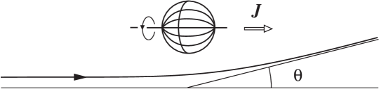
In this paper we extend the results of [10, 11] by computing, in the Born approximation, the scattering cross sections for fields of helicity $\pm\eta$ with $\eta=1/2{\rm~{}or~{}}2$ , i.e. for neutrinos and gravitational waves¹¹1After completing this work, we became aware of the article [12] in which, by using the Feynman-diagram technique, the cross sections for the gravitational scattering of photons and gravitons from a classical rotating body have been computed. In the electromagnetic case, we find a complete agreement. However, for gravitational wave scattering, the classical calculation of the present paper leads to a different prediction. The correctness of our result has been checked by using also the effective quantum field theory approach; we shall present the details in a forthcoming paper.. In the case of a gravitational deflection from a classical rotating body with mass $M$ and angular momentum $J$ (directed along the incident wavevector, see Figure 1), in the $\theta\rightarrow 0$ limit, the asymmetry turns out to be given by the following expression

\chi_{\eta}(\lambda,\theta)=\frac{(d\sigma_{+\eta}/d\Omega)-(d\sigma_{-\eta}/d\Omega)}{(d\sigma_{+\eta}/d\Omega)+(d\sigma_{-\eta}/d\Omega)}\simeq-\eta\frac{J}{Mc}\frac{2\pi}{\lambda}\theta^{2}

(1)

where $d\sigma_{\pm\eta}/d\Omega$ is the differential cross section for the scattering of $\pm\eta$ helicity waves, $\theta$ is the scattering angle and $\lambda$ denotes the wavelength. The validity of the Born approximation requires $4\pi^{2}GJ\theta\ll c^{3}\lambda^{2}$ . The helicity asymmetry as expressed in equation (1) is actually meaningful only for wavelengths sufficiently large so that diffraction effects are important. When this is not the case, i.e. for wavelengths $\lambda\ll 2\pi GM/c^{2}$ , the classical ray concept can meaningfully be used and the cross sections imply that the relation between the impact parameter and the deflection angle is modified as follows

\theta_{\pm\eta}(b)\simeq\theta_{0}(b)\left\{1-\eta\left(\frac{1}{4}\pm\frac{J}{Mc}\frac{2\pi}{\lambda}\right)\theta^{2}_{0}(b)|\ln\theta_{0}(b)|+O(\theta_{0}(b)^{3})\right\}

(2)

where $\theta_{0}(b)=4GM/(c^{2}b)$ is the standard result for the null geodesic deflection from a spherically symmetric body of mass $M$ . It should be noted that expressions (1) and (2) do not apply for $\lambda\rightarrow 0$ ; their domain of validity is discussed in section 3. We may thus conclude that, in analogy with the massive spinning (test) particle, massless spinning (test) particles do not move along null geodesics due to both a helicity-orbit coupling and to a helicity-spin coupling, corresponding respectively to the first and second term inside the round brackets in equation (2).

Refer to caption — Figure 1: Deflection from a rotating body.

The outline of the paper is as follows: in section 2 we compute the scattering cross sections in Born approximation for massless fields of helicity $\pm\eta=0,\pm 1/2,\pm 1,\pm 2$ . In section 3 we derive equations (1) and (2) and we discuss the range of application of these equations; finally, we give an estimate of the relevant effects in the case of deflections from the Sun and we discuss the case of large deflections in low frequency scattering off gravitationally compact objects. In the following we adopt relativistic field theory units $c=1=\hbar$ .

2 Scattering cross sections

2.1 Scalar field

In order to fix our notations and conventions, we begin with the scalar massless field; this will also be of help in separating the effects of “spin-orbit” coupling from the helicity couplings which we want to investigate in the following sections (the “spin” referred to is the angular momentum of the deflecting body).

To lowest order in the gravitational coupling constant, the metric tensor at large distance from a localized stationary rotating body in an otherwise empty spacetime can be put into the following form [13]:

	$\displaystyle g_{\mu\nu}dx^{\mu}dx^{\nu}$	$\displaystyle=$	$\displaystyle-\left(1-\frac{2GM}{\|\vec{x}\|}\right)dt^{2}+\left(1+\frac{2GM}{\|\vec{x}\|}\right)\delta_{ij}dx^{i}dx^{j}$		(3)
			$\displaystyle-4\epsilon_{ijk}\frac{GJ^{i}x^{j}}{\|\vec{x}\|^{3}}dt\,dx^{k}$		(3)

where multipoles of the body’s stress-energy tensor higher than the second are neglected, greek indices run from 0 to 3 with $t\equiv x^{0}$ , latin indices run from 1 to 3 and $\epsilon_{ijk}$ is the completely antisymmetric tensor. $M$ and $\vec{J}\equiv M\vec{S}$ are respectively the total mass and angular momentum of the body. The minimally coupled equation of motion for a massless scalar field $\phi(x)$ in curved spacetime can be written as [14]

0=\frac{1}{\sqrt{-|g|}}\partial_{\mu}\left(\sqrt{-|g|}g^{\mu\nu}\partial_{\nu}\phi\right)

(4)

where $|g|$ denotes the determinant of the covariant metric $g_{\mu\nu}$ and $g^{\mu\nu}$ is the inverse metric satisfying $g^{\mu\rho}g_{\rho\nu}=\delta^{\mu}_{\nu}$ . In the same approximations of equation (3), equation (4) becomes

-\eta^{\mu\nu}\partial_{\mu}\partial_{\nu}\phi=-\left(h^{\mu\nu}-\frac{1}{2}h^{\rho}{}_{\rho}\eta^{\mu\nu}\right)\partial_{\mu}\partial_{\nu}\phi

(5)

where $\nobreak{h_{\mu\nu}=g_{\mu\nu}-\eta_{\mu\nu}}$ and $\eta_{\mu\nu}=\eta^{\mu\nu}={\rm diag}(-1,1,1,1)$ denotes the flat Minkowski metric, which is used to raise and lower all indices. If one puts

\phi(x)=e^{ik_{\mu}x^{\mu}}\phi^{{\rm(in)}}+e^{-i\omega t}\phi^{{\rm(diff)}}(\vec{x})+\rm{c.c.}

(6)

with $k^{\mu}k_{\mu}=0,\,k^{0}=\omega$ , to lowest order in $G$ (Born approximation) the field $\phi^{{\rm(diff)}}$ satisfies the Helmoltz equation with a source term

-(\omega^{2}+\triangle)\phi^{{\rm(diff)}}(\vec{x})=k^{\mu}k^{\nu}h_{\mu\nu}(\vec{x})\,e^{i\vec{k}\cdot\vec{x}}\phi^{{\rm(in)}}\equiv F(\vec{k},\vec{x})

(7)

In the $|\vec{x}|\rightarrow\infty$ limit, this equation is asymptotically solved by [15]

\phi^{{\rm(diff)}}(\vec{x})\simeq\frac{e^{i\omega|\vec{x}|}}{|\vec{x}|}\int d^{3}y\,e^{-i\vec{p}\cdot\vec{y}}\frac{F(\vec{k},\vec{y})}{4\pi}\equiv\frac{e^{i\omega|\vec{x}|}}{|\vec{x}|}{\mathcal{A}}(\vec{k},\vec{p})

(8)

where $\vec{p}=\omega\vec{x}/|\vec{x}|$ is the asymptotic wave vector and the cross section for the scattering process $\vec{k}\rightarrow\vec{p}$ ( $\vec{k}$ is the incoming momentum, $\vec{p}$ the outgoing one) is given by

\frac{d\sigma_{\eta=0}}{d\Omega}=\left|\frac{{\mathcal{A}}}{\phi^{\rm(in)}}\right|^{2}

(9)

By putting all together one finds

{\mathcal{A}}(\vec{k},\vec{p})=\frac{GM}{\sin^{2}(\theta/2)}\left[1+\frac{i}{\omega}\vec{S}\cdot\vec{p}\times\vec{k}\right]\phi^{{\rm(in)}}

(10)

2.2 Neutrinos

Neutrinos are described in flat spacetime by massless fields transforming according to the $(1/2,0)$ or $(0,1/2)$ representations of $SL(2,\Cset)$ and their coupling to spacetime geometry is accomplished by introducing an orthonormal basis $\{\Theta_{I}^{\mu}\}$ on the tangent space, usually called tetrad or vierbein, so that [14]

g_{\mu\nu}(x)\Theta_{I}^{\mu}(x)\Theta_{J}^{\nu}(x)=\eta_{IJ}

(11)

where uppercase latin indices run from 0 to 3 and denote internal Lorentz indices. The spin connection is an $SL(2,\Cset)$ -valued connection defined by

\Omega^{IJ}_{\mu}\equiv\frac{1}{2}\left(E^{I}_{\rho}\nabla_{\mu}\Theta^{J\rho}-E^{J}_{\rho}\nabla_{\mu}\Theta^{I\rho}\right)

(12)

where $\{E^{I}_{\mu}\}$ is the cotetrad field satisfying

E^{I}_{\mu}(x)\Theta_{J}^{\mu}(x)=\delta^{I}{}_{J}

(13)

and Lorentz indices are raised an lowered with the Minkowski metric $\eta_{IJ}$ . Let $L$ be a $SL(2,\Cset)$ -valued gauge transformation

L:M\rightarrow SL(2,\Cset),x\mapsto L(x)

(14)

and let $[L_{(r)}]$ denote the matrix representing $L$ in the representation $(r)$ ; the tetrad is defined up to

\Theta_{I}^{\mu}(x)\rightarrow[L_{(\frac{1}{2},\frac{1}{2})}(x)]^{I^{\prime}}{}_{I}\Theta_{I^{\prime}}^{\mu}(x)

(15)

so that, if the field $\psi^{a}_{(r)}(x)$ transforms as

\psi_{(r)}(x)\rightarrow[L_{(r)}(x)]^{a}{}_{a^{\prime}}\psi^{a^{\prime}}_{(r)}(x)

(16)

and transforms as a scalar field under a change of coordinates, the derivative

D_{\mu}\psi_{(r)}^{a}\equiv\partial_{\mu}\psi_{(r)}^{a}-\frac{i}{2}\Omega_{IJ\mu}[J_{(r)}^{IJ}]^{a}{}_{a^{\prime}}\psi_{(r)}^{a^{\prime}}

(17)

transforms covariantly. The generators $[J_{(r)}^{IJ}]^{a}{}_{a^{\prime}}$ of $SL(2,\Cset)$ in the representation $(r)$ satisfy the commutation relations

[J_{(r)}^{IJ},J_{(r)}^{HK}]=i\left(\eta^{IH}[J_{(r)}^{JK}]+\eta^{JK}[J_{(r)}^{IH}]-\eta^{IK}[J_{(r)}^{JH}]-\eta^{JH}[J_{(r)}^{IK}]\right)

(18)

The propagation equation for neutrinos with helicity $\pm 1/2$ in flat spacetime can be written as

[\Gamma_{(\pm)}^{I}]^{a}{}_{a^{\prime}}\partial_{I}\psi_{(\pm)}^{a^{\prime}}=0

(19)

where $a$ is spinor index and

[\Gamma_{(\pm)}^{I}]^{a}{}_{a^{\prime}}=\begin{cases}\delta^{a}{}_{a^{\prime}}&{\rm for~{}}I=0\cr&\cr\pm[\sigma^{I}]^{a}{}_{a^{\prime}}&{\rm for~{}}I\neq 0\end{cases}

(20)

with $[\vec{\sigma}]^{a}{}_{a^{\prime}}$ the Pauli spin matrices; the $SL(2,\Cset)$ generators are given by

[J_{(\pm)}^{IJ}]^{a}{}_{a^{\prime}}=\begin{cases}\pm{\displaystyle\frac{i}{2}}[\sigma^{J}]^{a}{}_{a^{\prime}}&{\rm for~{}}I=0,\,J\neq 0\cr&\cr{\displaystyle\frac{\epsilon_{0}{}^{IJ}{}_{K}}{2}}[\sigma^{K}]^{a}{}_{a^{\prime}}&{\rm for~{}}I,J\neq 0\end{cases}

(21)

with $\epsilon_{0123}=1$ . The covariant field equations in a non flat spacetime are thus obtained by substituting the coordinate derivative $\partial_{I}$ in equation (19) with the covariant derivative $D_{I}\equiv\Theta^{\mu}_{I}D_{\mu}$ of equation (17) [14]:

[\Gamma_{(\pm)}^{I}]^{a}{}_{a^{\prime}}D_{I}\psi_{(\pm)}^{a^{\prime}}=0

(22)

To first order in $G$ , the tetrad and cotetrad fields can be put in the form

$\displaystyle\Theta_{0}^{\mu}$	$\displaystyle=$	$\displaystyle\left(1+\frac{GM}{\|\vec{x}\|}\right)\delta_{0}^{\mu}+\epsilon_{ijk}\frac{GJ^{j}x^{k}}{\|\vec{x}\|^{3}}\delta_{i}^{\mu}$
$\displaystyle\Theta_{i}^{\mu}$	$\displaystyle=$	$\displaystyle\left(1-\frac{GM}{\|\vec{x}\|}\right)\delta_{i}^{\mu}-\epsilon_{ijk}\frac{GJ^{j}x^{k}}{\|\vec{x}\|^{3}}\delta_{0}^{\mu}$
$\displaystyle E^{0}_{\mu}$	$\displaystyle=$	$\displaystyle\left(1-\frac{GM}{\|\vec{x}\|}\right)\delta^{0}_{\mu}+\epsilon_{ijk}\frac{GJ^{j}x^{k}}{\|\vec{x}\|^{3}}\delta^{i}_{\mu}$
$\displaystyle E^{i}_{\mu}$	$\displaystyle=$	$\displaystyle\left(1+\frac{GM}{\|\vec{x}\|}\right)\delta^{i}_{\mu}-\epsilon_{ijk}\frac{GJ^{j}x^{k}}{\|\vec{x}\|^{3}}\delta^{0}_{\mu}$

so that the spin connection $\Omega^{IJ}_{\mu}$ is given by

	$\displaystyle\Omega^{0i}_{\mu}$	$\displaystyle=$	$\displaystyle-\partial_{i}\left(\frac{GM}{\|\vec{x}\|}\right)\delta^{0}_{\mu}+\partial_{i}\left(\frac{\epsilon_{jhk}GJ^{h}x^{k}}{\|\vec{x}\|^{3}}\right)\delta^{j}_{\mu}$
	$\displaystyle\Omega^{ij}_{\mu}$	$\displaystyle=$	$\displaystyle-\partial_{i}\left(\frac{GM}{\|\vec{x}\|}\right)\delta^{j}_{\mu}+\partial_{i}\left(\frac{\epsilon_{jhk}GJ^{h}x^{k}}{\|\vec{x}\|^{3}}\right)\delta^{0}_{\mu}-(i\leftrightarrow j)$

and the propagation equation (22) becomes

	$\displaystyle 0$	$\displaystyle=$	$\displaystyle\partial_{t}\psi_{(\pm)}\pm[\vec{\sigma}]\cdot\vec{\nabla}\psi_{(\pm)}-\frac{G}{2}\vec{\nabla}\cdot\left(\frac{\vec{J}\times\vec{x}}{\|\vec{x}\|^{3}}\pm\frac{M\left[\vec{\sigma}\right]}{\|\vec{x}\|}\right)\psi_{(\pm)}$		(23)
			$\displaystyle+G\left(\frac{M}{\|\vec{x}\|}\mp\frac{\vec{J}\times\vec{x}\cdot[\vec{\sigma}]}{\|\vec{x}\|^{3}}\right)\partial_{t}\psi_{(\pm)}+G\left(\frac{\vec{J}\times\vec{x}}{\|\vec{x}\|^{3}}\mp M\frac{[\vec{\sigma}]}{\|\vec{x}\|}\right)\cdot\vec{\nabla}\psi_{(\pm)}$		(23)

Again, the field $\psi_{(\pm)}(x)$ can be written as the sum of an incident and a diffracted wave component

\psi_{(\pm)}(x)=e^{-i\omega t}\left[e^{i\vec{k}\cdot\vec{x}}\psi^{\rm(in)}_{(\pm)}+\psi^{\rm(diff)}_{(\pm)}(\vec{x})\right]

(24)

where $|\vec{k}|=\omega$ , and $\psi^{\rm(in)}_{(\pm)}$ satisfies

\vec{k}\cdot\left[\right.\!\vec{\sigma}\!\left.\right]\psi^{\rm(in)}_{(\pm)}=\pm\omega\,\psi^{\rm(in)}_{(\pm)}

(25)

To first order in the gravitational constant the diffracted component satisfies the equation

-i\omega\psi^{\rm(diff)}_{(\pm)}\pm[\vec{\sigma}]\cdot\vec{\nabla}\psi^{\rm(diff)}_{(\pm)}=F_{(\pm)}(\vec{k},\psi^{\rm(in)}_{(\pm)},\vec{x})

(26)

with

	$\displaystyle F_{(\pm)}(\vec{k},\psi^{\rm(in)}_{(\pm)},\vec{x})$	$\displaystyle=$	$\displaystyle iGM\omega\left[\frac{2}{\|\vec{x}\|}\mp\frac{\vec{S}\times\vec{x}}{\|\vec{x}\|^{3}}\cdot\left([\vec{\sigma}]\pm\frac{\vec{k}}{\omega}\right)\right]e^{i\vec{k}\cdot\vec{x}}\psi^{\rm(in)}_{(\pm)}$		(27)
			$\displaystyle+\frac{GM}{2}\vec{\nabla}\cdot\left(\frac{\vec{S}\times\vec{x}}{\|\vec{x}\|^{3}}\pm\frac{\left[\vec{\sigma}\right]}{\|\vec{x}\|}\right)e^{i\vec{k}\cdot\vec{x}}\psi^{\rm(in)}_{(\pm)}$		(27)

By left multiplying equation (26) with the operator $i\omega\pm[\vec{\sigma}]\cdot\vec{\nabla}$ one obtains

\left(\omega^{2}+\nabla^{2}\right)\psi^{\rm(diff)}_{(\pm)}=\left(i\omega\pm[\vec{\sigma}]\cdot\vec{\nabla}\right)F_{(\pm)}

(28)

The asymptotic $|\vec{x}|\rightarrow\infty$ solution to equation (28) is

$\displaystyle\psi^{\rm(diff)}_{(\pm)}(\vec{x})$	$\displaystyle\simeq$	$\displaystyle-\frac{e^{i\omega\|\vec{x}\|}}{\|\vec{x}\|}\int d^{3}y\frac{e^{-i\vec{p}\cdot\vec{y}}}{4\pi}\left(i\omega\pm[\vec{\sigma}]\cdot\vec{\nabla}\right)F_{(\pm)}(\vec{k},\psi^{\rm(in)}_{(\pm)},\vec{y})$	(29)
	$\displaystyle=$	$\displaystyle-i\frac{e^{i\omega\|\vec{x}\|}}{\|\vec{x}\|}\left(\omega\pm\vec{p}\cdot[\vec{\sigma}]\right)\int d^{3}y\frac{e^{-i\vec{p}\cdot\vec{y}}}{4\pi}F_{(\pm)}(\vec{k},\psi^{\rm(in)}_{(\pm)},\vec{y})$
	$\displaystyle\equiv$	$\displaystyle-i\frac{e^{i\omega\|\vec{x}\|}}{\|\vec{x}\|}\left(\omega\pm\vec{p}\cdot[\vec{\sigma}]\right){\mathcal{A}}_{(\pm)}(\vec{k},\psi^{\rm(in)}_{(\pm)},\vec{p})$

where $\vec{p}=\omega\vec{x}/|\vec{x}|$ is the outgoing momentum. The differential cross section for the scattering process $\vec{k}\rightarrow\vec{p}$ is thus given by

\frac{d\sigma_{\eta=\pm 1/2}}{d\Omega}={|(\psi^{\rm out}_{(\pm)})^{\dagger}{\mathcal{A}}_{(\pm)}|^{2}}

(30)

with $\psi^{\rm out}_{(\pm)}$ a constant spinor satisfying

\vec{p}\cdot[\vec{\sigma}]\psi^{\rm out}_{(\pm)}=\pm\omega\,\psi^{\rm out}_{(\pm)}\quad,\hskip 17.07182pt(\psi^{\rm out}_{(\pm)})^{\dagger}\psi^{\rm out}_{(\pm)}=\frac{4\omega^{2}}{(\psi^{\rm(in)}_{(\pm)})^{\dagger}\psi^{\rm(in)}_{(\pm)}}

(31)

Up to an irrelevant phase, equations (25) and (31) imply

	$\displaystyle(\psi^{\rm out}_{(\pm)})^{\dagger}\psi^{\rm(in)}_{(\pm)}$	$\displaystyle=$	$\displaystyle-2i\omega\cos(\theta/2)$		(32)
	$\displaystyle(\psi^{\rm out}_{(\pm)})^{\dagger}\left[\vec{\sigma}\right]\psi^{\rm(in)}_{(\pm)}$	$\displaystyle=$	$\displaystyle-\frac{i}{\omega\cos(\theta/2)}\left[i\vec{p}\times\vec{k}\pm\omega(\vec{p}+\vec{k})\right]$		(33)

so that a straightforward computation yields

	$\displaystyle(\psi^{\rm out}_{(\pm)})^{\dagger}{\mathcal{A}}_{(\pm)}$	$\displaystyle=$	$\displaystyle\frac{GM}{\sin^{2}(\theta/2)}\cos(\theta/2)\left[1+\frac{i}{2\omega}(\vec{S}\cdot\vec{p}\times\vec{k})\left(1+\frac{1}{\cos^{2}(\theta/2)}\right)\right.$		(34)
			$\displaystyle\hskip 99.58464pt\left.\mp\frac{1}{2}\tan^{2}(\theta/2)\vec{S}\cdot(\vec{k}+\vec{p})\right]$		(34)

2.3 Electromagnetic waves

The scattering cross section for electromagnetic waves has been computed in [10, 11] and we simply quote the result. For the process $(\vec{k},\vec{\epsilon}^{\rm\,(in)})\rightarrow(\vec{p},\vec{\epsilon}^{\rm\,(out)})$ one obtains

\frac{d\sigma_{\eta=1}}{d\Omega}=\frac{|{\mathcal{A}}(\vec{k},\vec{\epsilon}^{\rm\,(in)},\vec{p},\vec{\epsilon}^{\rm\,(out)})|^{2}}{(\vec{\epsilon}^{\rm\,(out)})^{*}\cdot\vec{\epsilon}^{\rm\,(out)}(\vec{\epsilon}^{\rm\,(in)})^{*}\cdot\vec{\epsilon}^{\rm\,(in)}}

(35)

with

	$\displaystyle{\mathcal{A}}(\vec{k},\vec{\epsilon}^{\rm\,(in)},\vec{p},\vec{\epsilon}^{\rm\,(out)})$	$\displaystyle=$	$\displaystyle\frac{GM}{\sin^{2}(\theta/2)}\left\{\left(\frac{1+\cos\theta}{2}+\frac{i}{\omega}\vec{S}\cdot\vec{p}\times\vec{k}\right)(\vec{\epsilon}^{\rm\,(out)})^{*}\cdot\vec{\epsilon}^{\rm\,(in)}\right.$		(36)
			$\displaystyle\hskip-28.45274pt\left.-\frac{1}{2\omega^{2}}(\epsilon^{\rm\,(out)}_{i})^{*}\epsilon^{\rm\,(in)}_{j}\left[k^{i}p^{j}+i\omega S^{h}q^{k}\left(\epsilon_{hki}p^{j}+\epsilon_{hkj}k^{i}\right)\right]\right\}$		(36)

where $\vec{q}=\vec{p}-\vec{k}$ .

2.4 Gravitational waves

The lowest order scattering of gravitational waves can likewise be computed by means of an expansion in powers of the gravitational constant, but since the scattering is actually induced by the self-interactions of the gravitational field, one needs to be more careful in writing the corresponding equations.

One can power expand the metric tensor and the energy momentum tensor as

	$\displaystyle g_{\mu\nu}(x)$	$\displaystyle=$	$\displaystyle\eta_{\mu\nu}+\ell\sum_{n=0}^{\infty}h^{(n)}_{\mu\nu}(x)\times\ell^{n}$		(37)
	$\displaystyle T_{\mu\nu}(x)$	$\displaystyle=$	$\displaystyle\sum_{n=0}^{\infty}T^{(n)}_{\mu\nu}(x)\times\ell^{n}$		(38)

where $\ell=\sqrt{G}$ (the extra $\ell$ factor in equation (37) has been introduced in order to give $h^{(0)}_{\mu\nu}$ the canonical dimensions of a free field). The Einstein equations

G_{\mu\nu}(g)=8\pi\ell^{2}T_{\mu\nu}

(39)

are likewise expanded, up to and including terms of order $\ell^{2}$ , as

$\displaystyle{\mathcal{G}}[h^{(0)}]$	$\displaystyle=$	$\displaystyle 0$	(40)
$\displaystyle{\mathcal{G}}[h^{(1)}]+{\mathcal{G}}^{\prime}[h^{(0)},h^{(0)}]$	$\displaystyle=$	$\displaystyle 8\pi T^{(0)}$	(41)
$\displaystyle{\mathcal{G}}[h^{(2)}]+2{\mathcal{G}}^{\prime}[h^{(1)},h^{(0)}]+{\mathcal{G}}^{\prime\prime}[h^{(0)},h^{(0)},h^{(0)}]$	$\displaystyle=$	$\displaystyle 8\pi T^{(1)}$	(42)

where ${\mathcal{G}}$ is the wave operator for a massless spin-2 field in Minkowski space:

{\mathcal{G}}[h]_{\mu\nu}=\frac{1}{2}\left[-h_{\mu\nu,\alpha}{}^{\alpha}-h^{\alpha}{}_{\alpha,\mu\nu}+h_{\alpha\mu,\nu}{}^{\alpha}+h_{\alpha\nu,\mu}{}^{\alpha}-\eta_{\mu\nu}\left(h^{\alpha\beta}{}_{,\alpha\beta}-h^{\alpha}{}_{\alpha,\beta}{}^{\beta}\right)\right]

Equations (40-42) admit a simple interpretation. Equation (40) describes free gravitational waves which propagate in flat Minkowski space and which encode the perturbative degrees of freedom of the gravitational field. Equation (41) describes the linearized gravitational field due to the energy momentum distribution of matter and of free gravitational waves. Note that, to this order, the energy momentum tensor $T^{(0)}_{\mu\nu}$ must satisfy the flat space conservation law $T^{(0)\mu\nu}{}_{,\nu}=0$ . Finally, equation (42) describes the lowest order correction to the gravitational wave propagation due to the linearized background as well as the backreaction on the matter distribution of the zeroth order gravitational wave, because $T^{(1)}$ must satisfy

T^{(1)\mu\nu}{}_{,\nu}=-T^{(0)\mu\lambda}\Gamma^{(0)\nu}{}_{\nu\lambda}-T^{(0)\lambda\nu}\Gamma^{(0)\mu}{}_{\nu\lambda}

(43)

In the limit of weak incoming gravitational waves, in equations (41) and (42) one can neglect the terms which are non linear in $h^{(0)}$ , so that, in order to obtain the lowest order scattering, we only need to compute ${\mathcal{G}}^{\prime}$ , which is given by [13]

	$\displaystyle{\mathcal{G}}^{\prime}[h,s]_{\mu\nu}$	$\displaystyle=$	$\displaystyle-\frac{1}{4}\left(\eta_{\mu\nu}h^{\alpha\beta}+h_{\mu\nu}\eta^{\alpha\beta}\right){\mathcal{R}}[s]_{\alpha\beta}-\frac{1}{4}\left(\eta_{\mu\nu}s^{\alpha\beta}+s_{\mu\nu}\eta^{\alpha\beta}\right){\mathcal{R}}[h]_{\alpha\beta}$		(44)
			$\displaystyle+\left(\delta^{\alpha}_{\mu}\delta^{\beta}_{\nu}-\frac{1}{2}\eta_{\mu\nu}\eta^{\alpha\beta}\right){\mathcal{R}}^{\prime}[h,s]_{\alpha\beta}$		(44)

with

$\displaystyle{\mathcal{R}}[h]_{\mu\nu}$	$\displaystyle=$	$\displaystyle\frac{1}{2}\left(-h_{\mu\nu,\alpha}{}^{\alpha}-h^{\alpha}{}_{\alpha,\mu\nu}+h_{\alpha\mu,\nu}{}^{\alpha}+h_{\alpha\nu,\mu}{}^{\alpha}\right)$
$\displaystyle{\mathcal{R}}^{\prime}[h,s]_{\mu\nu}$	$\displaystyle=$	$\displaystyle\frac{1}{4}\left[\frac{1}{2}h_{\alpha\beta,\mu}s^{\alpha\beta}{}_{,\nu}+h^{\alpha\beta}\left(s_{\alpha\beta,\mu\nu}+s_{\mu\nu,\alpha\beta}-s_{\alpha\mu,\beta\nu}-s_{\alpha\nu,\beta\mu}\right)\right.$	(45)
		$\displaystyle\hskip-28.45274pt\left.+h_{\nu}{}^{\alpha,\beta}\left(s_{\alpha\mu,\beta}-s_{\beta\mu,\alpha}\right)-\left(h^{\alpha\beta}{}_{,\beta}-\frac{1}{2}h_{\beta}{}^{\beta,\alpha}\right)\left(s_{\alpha\mu,\nu}+s_{\alpha\nu,\mu}-s_{\mu\nu,\alpha}\right)\right]$
		$\displaystyle\hskip-28.45274pt+h\leftrightarrow s$

Equations (40-42) become

$\displaystyle{\mathcal{G}}[h^{(0)}]$	$\displaystyle=$	$\displaystyle 0$	(46)
$\displaystyle{\mathcal{G}}[h^{(1)}]$	$\displaystyle=$	$\displaystyle 8\pi T^{(0)}$	(47)
$\displaystyle{\mathcal{G}}[h^{(2)}]$	$\displaystyle=$	$\displaystyle 8\pi T^{(1)}-2{\mathcal{G}}^{\prime}[h^{(1)},h^{(0)}]$	(48)

Let the incident wave be a transverse-traceless plane wave

h^{(0)}_{\mu\nu}(x)=\pi^{\rm(in)}_{\mu\nu}{\rm e}^{{\rm i}k^{\mu}x_{\mu}}+\rm{c.c.}

(49)

with $k^{\mu}k_{\mu}=\pi^{{\rm(in)}\mu}{}_{\mu}=0=k^{\mu}\pi^{\rm(in)}_{\mu\nu}$ . Since $T^{(0)}_{\mu\nu}$ is assumed to be stationary, one can choose an adapted coordinate system $\{x^{\mu}\}=\{t,\vec{x}\}$ in which $T^{(0)}_{\mu\nu,0}=0$ and the linearized Coulomb metric $h^{(1)}$ is given by

h^{(1)}_{\mu\nu}(\vec{x})=4\left(\delta^{\alpha}_{\mu}\delta^{\beta}_{\nu}-\frac{1}{2}\eta_{\mu\nu}\eta^{\alpha\beta}\right)\int\frac{T^{(0)}_{\alpha\beta}(\vec{x}^{\prime})}{|\vec{x}-\vec{x}^{\prime}|}d^{3}x^{\prime}

(50)

For a pointlike spinning body placed at rest on the origin of spatial coordinate, the zeroth order energy momentum tensor is

T^{(0)}_{\mu\nu}(t,\vec{x})=M\delta_{\mu}^{0}\delta_{\nu}^{0}\delta^{3}(\vec{x})-\frac{1}{2}(\delta_{\mu}^{0}\delta_{\nu}^{i}+\delta_{\nu}^{0}\delta_{\mu}^{i})\epsilon_{ijk}J^{j}\partial_{k}\delta^{3}(\vec{x})

(51)

and the metric $\eta_{\mu\nu}+Gh^{(1)}_{\mu\nu}(\vec{x})$ is precisely the metric of equation (3). Equation (43) is now solved by

T^{(1)}_{\mu\nu}=\left(\eta_{\nu\rho}\partial_{\mu}+\eta_{\mu\rho}\partial_{\nu}-\eta_{\mu\nu}\partial_{\rho}\right)\int d^{4}x^{\prime}\Gamma^{(0)\rho}{}_{\alpha\beta}(x^{\prime})T^{(0)\alpha\beta}(x^{\prime})G(x,x^{\prime})

(52)

with $G(x,x^{\prime})$ is a Green function for the 4-dimensional scalar wave operator (the ambiguity related to the particular choice of the Green function does not affect the scattering cross section of transverse traceless waves). Given the harmonic time dependence of $h^{(0)}$ and the stationarity of $T^{(0)}$ , one can set

h^{(2)}_{\mu\nu}=\left(\delta^{\alpha}_{\mu}\delta^{\beta}_{\nu}-\frac{1}{2}\eta_{\mu\nu}\eta^{\alpha\beta}\right)w_{\alpha\beta}(\vec{x}){\rm e}^{-{\rm i}\omega t}+\rm{c.c.}

(53)

with $\omega=k^{0}$ and $w_{0\mu}=0$ . With this choice, the $\mu=0=\nu$ and $\mu=0,\,\nu=i$ components of equation (48) yield respectively

	$\displaystyle w_{ii}(\vec{x})$	$\displaystyle=$	$\displaystyle-2\frac{D_{00}(\vec{x})}{\omega^{2}}$		(54)
	$\displaystyle w_{ij,j}(\vec{x})$	$\displaystyle=$	$\displaystyle 2{\rm i}\frac{D_{0i}(\vec{x})}{\omega}-2\frac{D_{00,i}(\vec{x})}{\omega^{2}}$		(55)

where

D_{\mu\nu}=-\left(8\pi T^{(1)}_{\mu\nu}-2{\mathcal{G}}^{\prime}[h^{(1)},h^{(0)}]_{\mu\nu}\right){\rm e}^{{\rm i}\omega t}

(56)

Finally, the space-space components of equation (48) yield the relevant equation for the scattering,

(\omega^{2}+\triangle)w_{ij}(\vec{x})=2\left(D_{ij}-\frac{D_{00,ij}}{\omega^{2}}+{\rm i}\frac{D_{0i,j}+D_{0j,i}}{\omega}\right)\equiv F_{ij}(\vec{k},\pi^{\rm(in)},\vec{x})

(57)

whose asymptotic $|\vec{x}|\rightarrow\infty$ solution is given by

w_{ij}(\vec{x})\simeq\frac{{\rm e}^{{\rm i}\omega|\vec{x}|}}{|\vec{x}|}\int d^{3}\!y\,{\rm e}^{-{\rm i}\vec{p}\cdot\vec{y}}\left(-\frac{F_{ij}(\vec{k},\pi^{\rm(in)},\vec{y})}{4\pi}\right)\equiv\frac{{\rm e}^{{\rm i}\omega|\vec{x}|}}{|\vec{x}|}{\mathcal{A}}_{ij}(\vec{k},\pi^{\rm(in)},\vec{p})

(58)

with $\vec{p}=\omega\vec{x}/|\vec{x}|$ .

The cross section for the gravitational scattering into gravitons with wavevector $\vec{p}$ and polarization $\pi^{{\rm(out)}}_{ij}$ , with $p_{i}\pi^{{\rm(out)}}_{ij}=0=\pi^{{\rm(out)}}_{ii}$ , is given by [16]

\frac{d\sigma_{\eta=2}}{d\Omega}=G^{2}\frac{\left|(\pi^{{\rm(out)}}_{ij})^{*}{\mathcal{A}}_{ij}\right|^{2}}{(\pi^{{\rm(out)}}_{ij})^{*}\pi^{{\rm(out)}}_{ij}(\pi^{{\rm(in)}}_{hk})^{*}\pi^{{\rm(in)}}_{hk}}

(59)

This expression shows that terms in $F_{ij}$ which either are total derivatives or are proportional to the metric tensor, such as $T^{(1)}$ , see equation (52), do not contribute to $d\sigma_{\eta=2}$ and need not be computed at all. Therefore

F_{ij}\sim\left(4{\mathcal{R}}^{\prime}[h^{(1)},h^{(0)}]_{ij}-h^{(0)}_{ij}\eta^{\alpha\beta}{\mathcal{R}}[h^{(1)}]_{\alpha\beta}\right){\rm e}^{{\rm i}\omega t}

(60)

and

	$\displaystyle\pi^{{\rm(out)}*}_{ij}{\mathcal{A}}_{ij}$	$\displaystyle=$	$\displaystyle\frac{M}{\sin^{2}(\theta/2)}\left[(\pi^{{\rm(out)}*}_{ij}\pi^{{\rm(in)}}_{ij})(1+\frac{{\rm i}}{\omega}\vec{S}\cdot\vec{p}\times\vec{k})\right.$		(61)
			$\displaystyle\hskip 28.45274pt\left.+\frac{{\rm i}}{\omega}(\pi^{{\rm(out)}*}_{ih}\pi^{{\rm(in)}}_{hj})(q_{i}\epsilon_{jpq}-q_{j}\epsilon_{ipq})S_{p}q_{q}\right]$		(61)

where $\,\vec{q}=\vec{p}-\vec{k}$ .

3 Gravitational helicity interaction

3.1 The helicity asymmetry

By rotating the spatial coordinates so that $\vec{k}=\omega\hat{z}$ and $\vec{p}=\omega(\cos\theta\hat{z}+\sin\theta\hat{x})$ , ( $\theta>0$ denotes the scattering angle) and by writing the amplitudes (36) and (61) in matrix form with respect to circular polarization states for the incident and scattered waves, one finds that helicity changing terms are exactly zero for $\eta=1/2$ and $\eta=1$ , while for $\eta=2$ they are $O(\theta^{4})$ with respect to the Rutherford amplitude; this is not unexpected, because, in the language of Feynman diagrams, the amplitude for scattering of gravitons off a massive (elementary) particle contains, besides the one-graviton-exchange graph which conserves helicity, also the “Compton” graph where the external gravitons couple directly to the massive particle (the total amplitude factorizes nicely, see [17]). The helicity conserving terms, on the other hand, are in general different from each other and in the $\theta\rightarrow 0$ limit the cross section for the scattering of $\pm\eta$ helicity waves is

\displaystyle\frac{d\sigma_{\pm\eta}}{d\Omega}(\vec{k},\vec{p})=\frac{G^{2}M^{2}}{\sin^{4}(\theta/2)}\left|1+i\omega S_{y}\theta-\frac{\eta}{2}\left(\frac{1}{4}\pm\omega S_{z}\right)\theta^{2}+O(\theta^{3})\right|^{2}

(62)

Expression (62) is valid for $\eta=0,1/2,1,2$ and summarizes the results contained in equations (9), (10), (30), (34), (35), (36), (59), (61). The meaning of the various terms, besides the usual Coulomb one, appearing in the right hand side of equation (62) can be understood as follows. The imaginary term $i\omega S_{y}\theta$ represents a “spin-orbit” interaction; it does not depend on the helicity of the scattered field and it merely couples the body’s angular momentum component which is orthogonal to the scattering plane to the orbital motion of the waves. This component is also present for scalar fields. The term $-\eta\theta/8$ does not depend on the sign of helicity and can be described as a “helicity-orbit” interaction because it is independent of the chirality of the wave and of the body’s angular momentum. Finally, the term $\mp\eta\omega S_{z}/2$ describes the effects of the “helicity-spin” interaction, which distinguishes the two chiralities.

The helicity asymmetry $\chi(\theta)$ at a deflection angle $\theta$ (such that $\omega S_{z}\theta^{2}\ll 1$ ) is thus

\chi_{\eta}(\lambda,\theta)=\frac{(d\sigma_{+\eta}/d\Omega)-(d\sigma_{-\eta}/d\Omega)}{(d\sigma_{+\eta}/d\Omega)+(d\sigma_{-\eta}/d\Omega)}\simeq-\eta\omega S_{z}\theta^{2}

(63)

which coincides with equation (1) and shows that a linearly polarized or unpolarized incident plane wave is detected at the deflection angle $\theta$ with a net nontrivial left circular polarization.

3.2 Orbit corrections

Let us now assume for simplicity that the incoming wave vector $\vec{k}$ is aligned with the angular momentum vector $\vec{J}$ , as shown in Figure 1; i.e. $\vec{k}\times\vec{J}=0$ and $\vec{k}\cdot\vec{J}=|\vec{k}||\vec{J}|$ . If diffraction effects are negligible, the semiclassical description of the scattering is valid. In this case, the $\theta\rightarrow 0$ limit of wave scattering admits a description in terms of particle orbits, where the dependence of the deflection angle $\theta$ on the impact parameter is given by [18]

\frac{d\sigma}{d\Omega}(\theta)=\frac{b(\theta)}{\sin\theta}\left|\frac{db(\theta)}{d\theta}\right|

(64)

By substituting equation (62) into equation (64) one finds

b_{\pm\eta}(\theta)=\frac{4GM}{\theta}\left\{1-\eta\left(\frac{1}{4}\pm\omega S_{z}\right)\theta^{2}|\ln\theta|+O(\theta^{3})\right\}

(65)

leading to expression (2) for the deflection angle $\theta_{\pm\eta}(b)$ at fixed impact parameter $b$ .

3.3 Domain of validity

We now discuss the range of application of equations (62), (1) and (2), which represent the main results of this paper. The propagation equation of the scattered waves can be interpreted as a Schroedinger equation describing the nonrelativistic scattering off an external potential, which is composed of a Newtonian part $\sim(1/r)$ and a dipole part $\sim(GJ/r)\nabla$ (see expression (3) and references [10, 11]). The criterion [19] of applicability of the Born approximation, which has been adopted in order to obtain equation (62), is known to fail for scattering off the Coulomb potential although the resulting amplitude turns out to be the exact one [18] (up to a phase). The remaining part $\sim(GJ/r)\nabla$ of the potential yields, for scattering at small angles, the condition

GJ\omega^{2}\theta\ll 1

(66)

On the other hand diffraction effects are negligible, and expression (64) is sensible, only if the condition

\omega\,b(\theta)\,\theta\gg 1

(67)

is met. When both (66) and (67) are satisfied, i.e.

\frac{1}{4GM}\equiv\omega_{\rm min}\ll\omega\ll\omega_{\rm min}\sqrt{\frac{4bM}{J}}\equiv\omega_{\rm max}(b)

(68)

equation (2) describes two kinds of corrections to the classical deflection computed by means of null geodesics. A distant object emitting unpolarized radiation of the kinds discussed here should form, if a rotating body lies between the object and the observation point, distinct images for each kind of radiation: for waves of helicity $\pm\eta$ , equation (2) predicts two images of equal intensity with an angular separation given by

\Delta\theta_{\eta}(b)\simeq 2\eta\omega\frac{J}{M}\theta_{0}^{3}(b)|\ln\theta_{0}(b)|

(69)

and centered around the deflection angle

\theta_{\eta}(b)\simeq\theta_{0}(b)\left\{1-\frac{\eta}{4}\theta_{0}^{2}(b)|\ln\theta_{0}(b)|\right\}

(70)

In the case of the Sun, with an impact parameter $b\simeq 1.5\times 10^{9}\,$ m (twice the radius of the Sun) and with $J\simeq 1.63\times 10^{41}\,{\rm kg\,m^{2}\,s^{-1}}$ [20], one finds $\theta_{0}\simeq 4\times 10^{-6}$ , $\omega_{\rm min}=5\times 10^{4}\,$ Hz and $\omega_{\rm max}=2.35\times 10^{8}\,$ Hz, so that the differential angular displacement between the helicity $\eta$ and the “geodesic” ( $\eta=0$ ) images of the distant object turns out to be

\frac{\theta_{0}-\theta_{\eta}}{\theta_{0}}\simeq 5\,\eta\times 10^{-11}

(71)

while the differential displacement between the images of the two chiral components is

\frac{\Delta\theta_{\eta}}{\theta_{0}}\simeq 3.6\,\eta\,\omega({\rm Hz})\,\times 10^{-16}

(72)

In the practical case of Earth based observers, the angular momentum vector of the Sun will not be directed as the incoming radiation and equation (64) cannot apply because the cross section (62) gets a nontrivial azimuthal dependence. This dependence can be integrated over in order to obtain an average deflection angle at a given impact parameter; in this case, equations (69) and (70) become respectively

\langle\Delta\theta_{\eta}\rangle(b)\simeq 2\eta\omega\frac{J\cos\phi}{M}\theta_{0}^{3}(b)|\ln\theta_{0}(b)|

(73)

and

\langle\theta_{\eta}\rangle(b)\simeq\theta_{0}(b)\left\{1+\left[\left(\frac{\omega J\sin\phi}{M}\right)^{2}-\frac{\eta}{4}\right]\theta_{0}^{2}(b)|\ln\theta_{0}(b)|\right\}

(74)

where $\cos\phi=\vec{J}\cdot\vec{k}/(J\omega)$ .

Equations (73) and (74) are not guaranteed to work for $\omega\gtrsim\omega_{\rm max}$ , but assuming they do, the null experiment of Harwit et al. [21] can be given a quantitive description. In fact, Harwit et al. studied electromagnetic radiation $(\eta=1)$ with $\omega\simeq 50\,$ GHz and $b\simeq 5.5\times 10^{9}\,$ m, leading to $\omega_{\rm max}\simeq 4.5\times 10^{8}\,$ Hz. According to the Born approximation result (72), the expected effect is

\frac{\Delta\theta_{\eta=1}}{\theta_{0}}\simeq 1.5\cos\phi\times 10^{-6}

(75)

which is indeed at least two orders of magnitude below the $10^{-4}$ accuracy they had ( $\,|\cos\phi\,|\lesssim 0.12\,$ ). The magnitude (75) of the expected deviation from the geometric optics approximation is much larger than the estimate $\Delta\theta_{\eta=1}/\theta_{0}\lesssim 10^{-18}$ presented in [9].

For frequencies $\omega\lesssim\omega_{\rm min}$ the orbit approximation fails to be reliable because the diffraction effects become important and the helicity interaction manifests itself in the helicity asymmetry of equation (1).

3.4 Scattering at large angles

The preceding discussion was limited to the near-forward scattering region $\theta\sim 0$ , where the Born approximation can be trusted. Large gravitational deflections are generated by very compact objects with size close to the gravitational radius, so that nonlinear GR effects are presumably important. One should then resort to more sophisticated methods such as wave decomposition into radial and spherical modes [22]. For spherically symmetric spacetimes ( $J=0$ ), the proper perturbation expansion parameter for propagation of modes with orbital angular momentum number $\ell$ is given by $GM\omega/\ell$ , so that, for large deflections (i.e. low values of $\ell$ ), the use of the linearized metric of equation (3) is justified in the diffraction limit $\omega\ll\omega_{\rm min}$ . Note that for black holes this inequality automatically enforces the validity of relation (66) for $\theta=O(1)$ .

In the diffraction limit, equations (34), (36), (61) can thus be trusted for all values of $\theta$ . We see in particular that for $\eta\neq 0$ the backward cross section for helicity conserving scattering vanishes (no glory effect) when the incident wave vector is aligned with the angular momentum of the deflecting body. This is also the case for high frequency scattering, which is best described by the JWKB approximation [23, 24]. Note that for $\eta=1,2$ the glory for helicity conserving processes is absent whether or not the incident wave vector is aligned to $\vec{J}$ . However, while for $\eta=1/2,1$ the helicity changing amplitudes vanish, this is not the case for $\eta=2$ —as mentioned before— and the symmetry argument leading to the absence of glory effect for $\eta\neq 0$ [23] cannot apply to these processes. Indeed, equation (61) shows that the helicity changing glory scattering cross section of gravitons is nonvanishing, in agreement with the analysis of the scattering from Schwarzschild and Kerr black holes [22].

We wish to thank S. Degl’Innocenti and S. Shore for useful discussions.

References

[1] M. Mathisson, Acta Physica Pol. 6 167 (1937).
[2] A. Papapetrou, Proc. R. Soc. Lond. 209 248 (1951).
[3] R. Wald, Phys. Rev. D 6, 406 (1972).
[4] B. Mashhoon, Ann. Phys. (N.Y.) 89, 254 (1975).
[5] G.B. Skrotskii, Dokl. Acad. Nauk SSSR 114, 73 (1957).
[6] N.L. Balazs, Phys. Rev. 110, 236 (1958).
[7] J. Plebanski, Phys. Rev. 118, 1396 (1960).
[8] B. Mashhoon, Phys. Rev. D 7, 2807 (1973).
[9] B. Mashhoon, Nature 250, 316 (1974).
[10] E. Guadagnini, Phys. Lett. B 548, 19 (2002).
[11] A. Barbieri and E. Guadagnini, Nucl. Phys. B 703, 391 (2004).
[12] W.K. De Logi and S.J. Kovács Jr., Phys. Rev. D 16 237 (1977).
[13] C.W. Misner, K.S. Thorne and J.A. Wheeler, Gravitation, Freeman (New York, 1973).
[14] N.D. Birrel and P.C. Davies, Quantum fields in curved space, Cambridge University Press (Cambridge, 1982).
[15] J.D. Jackson, Classical electrodynamics, Wiley (New York, 1975).
[16] S. Weinberg, Gravitation and cosmology: principles and applications of the general theory of relativity, Wiley (New York, 1972).
[17] S.Y. Choi, J.S. Shim and H.S. Song, Phys. Rev. D 51, 2751 (1995)
[18] L. Landau and E. Lifchitz, Mécanique Quantique, Éditions Mir (Moscou, 1966).
[19] R.G. Newton, Scattering Theory of Waves and Particles, Springer-Verlag (New York, 1982).
[20] A. Cox and C.W. Allen, Allen’s astrophysical quantities, Springer-Verlag (New York, 2000).
[21] M. Harwit et al., Nature 249, 230 (1974).
[22] J.A.H. Futterman, F.A. Hamndler and R.A. Matzner, Scattering from black holes, Cambridge University Press (Cambridge, 1988).
[23] B. Mashhoon, Phys. Rev. D 10, 1059 (1974).
[24] R.A. Matzner, C. DeWitte-Morette, B. Nelson and T.-R. Zhang, Phys. Rev. D 31, 1869 (1985).