Report on the first binary black hole inspiral search in LIGO data

Abstract

The LIGO Scientific Collaboration is currently engaged in the first search for binary black hole inspiral signals in real data. We are using the data from the second LIGO science run and we focus on inspiral signals coming from binary systems with component masses between 3 and 20 solar masses. We describe the analysis methods used and report on preliminary estimates for the sensitivities of the LIGO instruments during the second science run.

1 Introduction

The Laser Interferometer Gravitational Wave Observatory (LIGO) consists of three Fabry-Perot-Michelson interferometers: a 4 km interferometer at Livingston (hereafter L1), a 4 km interferometer at Hanford (hereafter H1) and a 2 km interferometer also at Hanford (hereafter H2). Those instruments are very close to the end of the commissioning phase and are approaching their design sensitivities as of December 2004. The second science run (hereafter S2) of the LIGO intereferometers took place from February 14 to April 14, 2003. During that run all three LIGO interferometers were operated in “science mode”, stably and in coincidence. Even though the design sensitivity goal had not been achieved at that time, the data acquired represent the best broad-band sensitivity to gravitational waves that had been achieved up to that date.

We report here on the search for gravitational waves from non-spinning binary black hole inspirals in the data from the second science run. For that search we take advantage of the knowledge acquired via the binary neutron star inspiral search and we use methods developed for it. However, we have to address issues that are unique to binary black hole inspirals.

2 Target sources

The target sources for the search described in this paper are binary black hole systems with component masses equal to a few times the mass of the sun. The intrinsic angular momentum of each component of the binary is not taken into account. The effects of it will be examined in future searches.

Black hole binaries are believed to emit gravitational waves during all stages of their evolution, namely the inspiral, the merger and the ringdown. There are no reliable models for the waveform of the merger phase at present. Numerical work [1, 2] has given insights into the merger problem and the progress in numerical relativity indicates that models for the merger phase will be developed in the future. At this time, it is more appropriate to search for binary black hole mergers using techniques developed for finding unmodeled bursts [3]. Additionally, even though there are theoretical waveforms for the ringdown phase, we do not search for ringdowns, for reasons that are explained below. Thus, we focus on the gravitational waves emitted during the inspiral phase.

At the first stages of the inspiral there is only small loss of energy per orbit and the standard post-Newtonian approximation for calculating the gravitational waves emitted is applicable. As the separation between the two black holes becomes smaller, relativistic effects become more significant and the standard post-Newtonian approach becomes less accurate. That specifically happens as the “innermost stable circular orbit” (or ISCO) is approached, namely the last orbit before the highly non-adiabatic plunge of the black holes towards each other begins. The higher the masses of the two black holes, the earlier the ISCO is reached. The test-mass approximation gives that the ISCO frequency can vary from 55 Hz for a system of two black holes with component masses equal to 40 $M_{\odot}$ up to 733 Hz for a system of two black holes with component masses equal to 3 $M_{\odot}$.

Various different approaches based on post-Newtonian calculations [4, 5, 6, 7] have been followed in order to solve the difficult problem of the late-time evolution of the inspiral phase of binary black hole systems. These approaches differ in the approximation methods used to evolve the system as it nears the ISCO and on the predicted ISCO frequency. Consequently, they also differ in their predictions for the gravitational waveforms emitted by the system at the last stages of the inspiral phase, when the frequency is approaching the ISCO frequency.

A low-frequency cutoff of 100 Hz needed to be imposed on the S2 data, for reasons that will be explained in sec. (4). That cutoff limited the masses of the binary systems for which we could detect an inspiral signal within the LIGO band: we had to focus the search on binary black hole systems with component masses between 3 and 20 $M_{\odot}$. (The lowest ISCO frequency for that mass range is that for the 20 - 20 $M_{\odot}$ system, equal to 110 Hz according to the test-mass approximation, just above the imposed low-frequency cutoff.) For these binaries the expected ringdown frequencies range from 295 Hz to 1966 Hz [8], mostly in the low-sensitivity frequency band of LIGO during S2. That is the reason why we do not search for the ringdown phase of those binaries.

3 Templates and filtering

The low-frequency cutoff imposed on the data does not only restrict the mass range for this search but it also implies that for the black hole binaries of total mass close to 40 $M_{\odot}$ the LIGO interferometers were sensitive only to the very last part of the inspiral phase, during S2. As was mentioned in sec. (2), the various theoretical models produce different predictions and waveforms for that part of the evolution of the system. Given that fact, we are faced with the dilemma of which one of the physical waveforms to implement in the matched filtering code that we use to search the data for inspiral signals. Since some of those waveforms differ significantly with each other (and potentially with an actual gravitational waveform), choosing one that does not match well with the real inspiral gravitational wave signal may hurt the efficiency of the search.

Alternatively, we choose to filter the data using a family of waveform templates which were developed specifically for detection of binary black hole inspirals. Those templates were first described in a recent paper by Buonanno, Chen and Vallisneri [9] and are usually referred to as BCV templates. The BCV templates are phenomenological templates because they are not derived by calculating the evolution of the binary system according to a specific physical model. However, their phase evolution and amplitude are based on the post-Newtonian phase evolution and amplitude. They have a high match with most physical waveform templates that have been proposed in the literature and are known to be efficient at identifying inspiral gravitational wave chirps in the data. Their frequency-domain form is

$$\tilde{h}(f)=f^{-7/6}\;(1-\alpha f^{2/3})\;\theta(f_{\mathrm{cut}}-f)\;e^{i(2\pi ft_{0}+\phi_{0}+\psi_{0}f^{-5/3}+\psi_{3}f^{-2/3})}.$$ (1)

The amplitude component $f^{-7/6}$ is the standard restricted Newtonian amplitude. The component $(\alpha\;f^{-1/2})$ is designed to capture any post-Newtonian amplitude corrections and to obtain high matches with non-adiabatic models that deviate from the Newtonian amplitude in the last parts of the inspiral and the merger. The parameters $t_{0}$ and $\phi_{0}$ are the time of arrival and phase of the waveform. The parameters $\psi_{0}$ and $\psi_{3}$ are phenomenological parameters governing the frequency evolution of the chirp, with values that are related to the masses of the component black holes. In order to obtain high matches with the various post-Newtonian models that predict different terminating frequencies, the cutoff frequency $f_{\mathrm{cut}}$ is imposed to terminate the waveform.

We filter the Fourier-transformed data $\tilde{s}(f)$ with a template $\tilde{h}(f)$ and construct the signal-to-noise ratio. In general that is given by

$$\rho(h)=\frac{<s,h>}{\sqrt{<h,h>}}$$ (2)

where the inner product is defined as

$$<s,h>=4\Re\int_{0}^{\infty}\frac{\tilde{s}(f)\;\tilde{h}^{\ast}(f)}{S_{h}(f)}df.$$ (3)

In eq. (3), $S_{h}(f)$ is the one-sided noise power spectral density. Specifically for the BCV templates, we construct a bank of templates for the intrinsic parameters $\psi_{0}$, $\psi_{3}$ and $f_{\mathrm{cut}}$ and we maximise the signal-to-noise ratio over the extrinsic parameters $t_{0}$, $\phi_{0}$ and $\alpha$.

A standard part of the matched filtering process is the $\chi^{2}$-test [10]. This test quantifies the degree to which the signal-to-noise ratio is distributed in time in accordance to the way it would be distributed for a true gravitational wave inspiral chirp. It is very efficient at distinguishing binary neutron star inspiral signals from loud non-gaussian noise bursts in the data and is used in the binary neutron star inspiral search. However, we found that test to not be applicable to the search for gravitational waves from binary black hole inspirals in the S2 data. The expected short duration and small number of cycles in the S2 LIGO frequency band for many of the possible binary black hole inspiral signals made such a test unreliable unless a very loose threshold were to be set. A loose threshold, on the other hand, resulted in only a minimal reduction in the number of instrumental noise events picked up. That and the fact that the $\chi^{2}$-test is computationally costly made us decide to not use it in this search.

4 Analysis pipeline and trigger generation

In order to search the data for binary black hole inspiral gravitational waves we have developed a multi-level pipeline. The pipeline is described in great detail in [11, 12]. Technical issues such as segmentation of the data and power spectrum estimation are discussed in those papers and our choices for the related parameters are explained. For completeness, a brief explanation of the main features of the pipeline is given here.

In order to increase the confidence that an event that comes out of the pipeline is a real gravitational wave as opposed to an event due to instrumental noise, we choose to search only S2 data acquired during times when the L1 interferometer and at least one of the two Hanford interferometers were operating in science mode. That allows us to test the events that come out of the pipeline for coincidence between the Hanford and Livingston sites. We choose to not search data from times when both H1 and H2 (but not L1) were operating in science mode, due to the fact that noise bursts caused by environmental disturbances may be correlated between H1 and H2 and may appear as coincident events at the end of our pipeline. We then have three data sets to consider, based on which of the two Hanford interferometers were operating: data from times when L1 and only H1 were operating (L1-H1 double coincident data), data from times when L1 and only H2 were operating (L1-H2 double coincident data) and data from times when L1 and both H1 and H2 were operating (L1-H1-H2 triple coincident data).

Various data quality cuts were imposed in order to make sure that the data was appropriate for our analysis. Detailed investigations resulted in us imposing the 100 Hz low-frequency cutoff mentioned in sec. (2). That cutoff was necessary in order to eliminate the non-stationary noise that was present at frequencies around 70 Hz and was resulting in a lot of spurious instrumental noise events being observed on the data. We expect to lower this low-frequency cutoff in the analysis of future science runs.

The data is broken up to “analysis segments” of 2048 s for power spectrum estimation and for matched filtering. One fundamental feature of the pipeline is the fact that we perform a triggered search. During the second science run, the L1 interferometer was more sensitive than either of the Hanford interferometers. More information on this will be given in sec. (5). Given that and the fact that the L1 interferometer is nearly aligned with the Hanford interferometers, we expect that in most cases gravitational waves observable in H1 and/or H2 are also observable in L1. For that reason, we choose to start the triggered search by creating a template bank over the parameters $\{\psi_{0},\;\psi_{3},\;f_{\mathrm{cut}}\}$ for each 2048-s analysis segment of the L1 interferometer. The number of templates in the bank varies with the variations in the noise but is typically about 1000 templates. The L1 data is filtered with that bank and the times, phases, $\alpha$ and template parameters for which the signal-to-noise ratio exceeds the threshold of 7 are recorded as “triggers”. All the corresponding triplets $\{\psi_{0},\;\psi_{3},\;f_{\mathrm{cut}}\}$ form the “triggered” template bank with which the data from the second interferometer (H1 for the L1-H1 and the L1-H1-H2 data or H2 for the L1-H2 data) is then filtered. The next step is the coincidence step. We test if the triggers from the two sites have consistent parameters and we reject those that do not. Specifically, we test that the times of the triggers at the two sites differ by no more than the travel time of gravitational waves between the two sites (10 ms) plus the accuracy by which we can recover the end time of the gravitational wave signals (10 ms), i.e. we require the trigger times at the two sites to be within $\pm$ 20 ms of each other. We also test that the template parameters of the triggers are equal for the time-coincident triggers that come from the two sites. For the cases of double coincident data (L1-H1 or L1-H2) the coincident triggers are recorded at this point. For the case of triple coincident data, the triggers that survive L1-H1 coincidence are used to create a second triggered bank with which the data from the H2 interferometer is filtered. The H2 triggers are tested for coincidence with the L1 and H1 triggers generated for the same triple coincident data. However, given the limited sensitivity of the H2 interferometer, we keep all the L1-H1 coincident triggers regardless of whether they are coincident with any H2 triggers or not. We end up with either double or triple coincident triggers for the triple coincident data. The final step of the pipeline is the clustering of the triggers. Clustering the triggers is necessary because both strong noise bursts and strong gravitational wave signals are known to give large numbers of triggers with different coalescence times and filter parameters, which are difficult to handle in the follow-up analysis. We choose to cluster the triggers that occur within intervals of 250 ms, approximately half the duration of the longest possible binary black hole inspiral signal that we can detect in the S2 data given the low-frequency cutoff of 100 Hz.

Finally, it should be noted that the various parameters of the pipeline (signal-to-noise ratio threshold, coincidence time window, etc.) were determined by adding simulated inspiral signals in the data and trying to recover them with our pipeline. The tuning was done on a part of the S2 data (approximately 10%) that was predetermined and representative of all the data from the second science run. That subset of data is referred to as “playground” data.

5 Monte-Carlo simulations

In order to tune the various parameters of the pipeline, to validate the pipeline and to verify that if there is a detectable signal in the data we would be able to identify it, we perform Monte Carlo simulations during which we add simulated binary black hole inspiral signals into the data stream (in software) and try to recover them with our pipeline. Monte-Carlo simulations also allow us to determine the efficiency of our pipeline at detecting binary black hole inspiral signals. The added simulated signals are referred to as “injections”.

5.1 Characteristics of injected signals

As was mentioned in sec. (3), the templates that we use for the matched filtering step of the pipeline are phenomenological templates which do not result from calculations based on physical models. However, for the signals that we inject in the data, we use waveforms that are based on physical models. Of the large number of physical waveforms available in the literature, we choose to inject effective-one-body (EOB) [7], standard post-Newtonian (spN) [5] and PadeT1 waveforms (PT1) [6], all of second post-Newtonian order. In addition to validating and measuring the efficiency of our pipeline, the fact that we inject different physical waveforms allows us to determine how effective the BCV templates are at identifying signals that are based on different models.

In the case of neutron star binaries there are theoretical population models that are based on radio observations of such systems. Those models restrict the presence of binary neutron stars into galaxies and give possible mass distributions for them. In contrast, binary black hole systems can only be detected via the gravitational waves that they generate and have never been observed before. Thus there are no observation-based theoretical models for their population. For that reason the binary black hole simulated signals are not placed only inside galaxies but are spread throughout space.

The choice for the distances of the simulated signals is based on the S2 sensitivities of the LIGO instruments. Specifically to binary black hole inspirals, theoretical calculations using the standard post-Newtonian waveforms showed that given the actual S2 power spectra for the three instruments, the distance at which an optimally oriented 5 - 5 $M_{\odot}$ binary inspiral would be detected with a signal-to-noise ratio of 8 (effective range) varied from 4 to 7 Mpc for L1, 2 to 3 Mpc for H1 and 1 to 2 Mpc for H2. In fact the effective range increased for all three interferometers as the run was progressing. Due to the large range of ISCO frequencies for the black hole binaries we consider, these ranges can be quite different for different signal-to-noise ratios and different masses of the systems. Binaries of total mass close to 6 $M_{\odot}$ do not have enough power in band and will not be detectable at distances as large as the effective ranges mentioned above. Binaries of total mass close to 40 $M_{\odot}$ do not have many cycles in the S2 LIGO frequency band and will also not be detectable at distances as large as the effective ranges mentioned above. On the other had, binaries of total mass around 20 $M_{\odot}$ have enough power in band and can be expected to be detectable at distances larger than the effective ranges previously mentioned.

For our initial simulations we choose to inject signals the distance of which varies between 100 kpc and 10 Mpc. The random sky angles and orientations of the binaries result in some signals having much larger effective distances. Populations of distances as low as 10 kpc and as high as 20 Mpc will also be injected, but the results are not presented here. Various choices for the distance distribution were considered. It was determined that choosing a uniform-distance distribution or a uniform-volume distribution would overpopulate the region of large distances (where the instruments were not very sensitive) and would result in very few injections with small and intermediate distances (for which we are more interested in measuring the efficiency of our pipeline). For those reasons we choose a distribution that has uniform $\log$(distance).

We limit the component masses of the binaries for the simulated signals between 3 and 20 $M_{\odot}$. That choice was justified in sec. (2). We inject populations with uniform component mass between 3 and 20 $M_{\odot}$ as well as populations with uniform total mass between 6 and 40 $M_{\odot}$ with each component mass between 3 and 20 $M_{\odot}$. The results presented here are for the latter choice.

5.2 Analysis of Monte-Carlo simulations

We report here on injections performed on the playground part of the S2 data. The efficiency for recovering the injected waveforms (number of found injections of a given distance divided by the total number of injections of that distance) is shown in fig. (1).

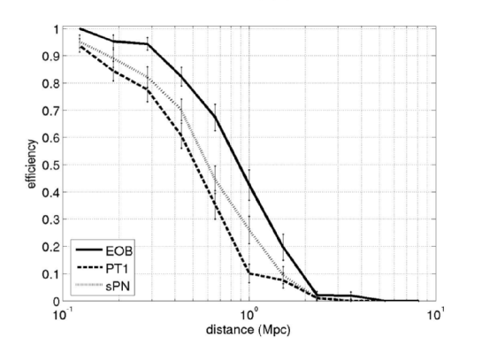
Figure 1: The efficiency versus the distance for the three families of injected waveforms is shown. The binomial error bars are also shown.

The first interesting result is that we can detect gravitational waves from binary black hole inspirals with efficiency of at least 10% at distances of 1 Mpc, for the mass range that we are exploring. That is consistent with the expected reach of the LIGO interferometers during S2. The fact that some injected signals are missed at distances lower than the effective range mentioned in sec. (5.1) can be attributed to various factors. Some of the injected signals have highly non-optimal orientation for at least one of the LIGO interferometers and can only produce triggers with signal-to-noise ratio lower than the threshold. Other signals, injected at times early during S2, correspond to epochs during which the reach of the LIGO interferometers was limited. Finally, some signals correspond to very low or very high masses and thus are not expected to be detectable at distances as large as the effective ranges mentioned previously.

The second interesting result pertains to the efficiency of our pipeline for different injected waveforms. It is clear from fig. (1) that the efficiency for recovering EOB waveforms is higher than that for standard post-Newtonian or PadeT1 waveforms, for all distances. The efficiency of recovering standard post-Newtonian waveforms is a little higher than the efficiency for recovering PadeT1 waveforms. That is consistent with the observation [9] that the BCV templates have higher overlap with the EOB waveforms than with the standard post-Newtonian or the PadeT1 waveforms.

6 Background estimation

We estimate the rate of accidental coincidences (also known as background rate) for this search by introducing an artificial time offset (lag) $\Delta t$ to the triggers coming from the Livingston detector relative to the Hanford detectors. The time-lag triggers are fed into the coincidence steps of the pipeline and, for triple coincident data, to the step of the filtering of the H2 data and the last coincidence. For a given time lag, the triggers which emerge from the end of the pipeline are considered as one single trial representation of an output from a search if no signals are present in the data. By choosing a lag of more than 20 ms (equal to the time coincidence window between the two sites), we ensure that a true gravitational wave could never produce coincident triggers in the time-shifted data streams. To avoid correlations, we use lags longer than the duration of the longest waveform ($\sim$ 0.6 s). We choose to not time-shift the two Hanford detectors relative to one another since there may be real correlations due to environmental disturbances between them. The resulting triggers are not correlated at the sites and so they correspond only to accidental coincidences of noise triggers.

6.1 Background result

A total of 80 time-lags were analyzed to estimate the background. Specifically the values of the time shifts ranged from $\Delta t=-407\;s$ up to $\Delta t=+407\;s$ in increments of $10\;s$. The time lags of $\pm 7s$ were not performed. We focus here on the signal-to-noise ratio for the triggers from each detector: $\rho_{\mathrm{L}}$ for L1 and $\rho_{\mathrm{H}}$ for the Hanford detectors.

The distribution of time-lag triggers in the $(\rho_{\mathrm{L}},\rho_{\mathrm{H}})$ plane is shown in fig. (2). The accidental coincidence triggers are plotted as dots in that graph. There is a concentration of those triggers at the lower left corner of the graph, which corresponds to the region of low signal-to-noise ratio for all detectors. There are also “tails” in the distribution, that correspond to triggers that have high signal-to-noise ratio in one detector and low signal-to-noise ratio in the other. The distribution is quite different from the equivalent distribution that was observed in the binary neutron star search [11], where those tails of triggers were not present. The presence of these tails (and their absence from the corresponding distribution in the binary neutron star case) can be attributed to the fact that the $\chi^{2}$-veto was not applied in this search and thus some of the loud instrumental noise bursts that would have been eliminated by that test have instead survived.

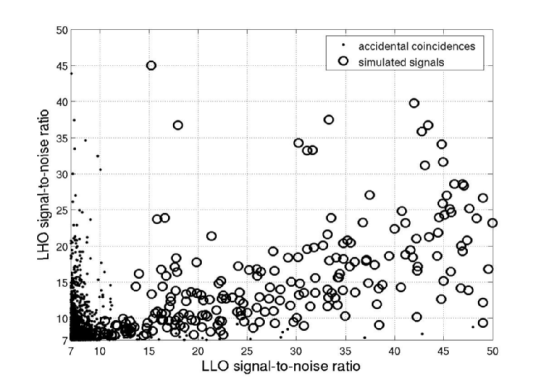
Figure 2: The accidental coincidences from the time-shifted triggers (dots) and the triggers from the simulated signal injections (open circles) are shown.

6.2 Comparison of injections to the background

It is interesting to compare the accidental coincidence triggers with triggers that result by recovering simulated inspiral signals added on the data. The triggers from the simulated signals are also plotted in fig. (2) as open circles.

The distributions of the two types of triggers are quite different. The injection triggers cluster mainly in the region under the diagonal of the $\rho_{\mathrm{H}}$ versus $\rho_{\mathrm{L}}$ plane. That is due to the fact that, as was mentioned in sec. (4), the L1 interferometer was more sensitive than either of the Hanford interferometers during S2. Consequently, signals that are detected at both sites have a higher signal-to-noise ratio in L1 than in H1 or H2. The few injection triggers that are above the diagonal correspond to injected signals from binary systems that are favorably oriented for H1 and H2 but not so for L1, which results to them having a higher signal-to-noise ratio at the Hanford instruments.

7 Summary

We described the methods used and the preliminary results of the first search for binary black hole inspirals that has been performed in real data. This search, even though similar in some ways to the binary neutron star inspiral search, has some significant differences and presents unique difficulties. The methods discussed in this paper are being used to complete the search in the S2 data and have given us insight on issues related to the spinning binary black hole search being performed on the data from the third science run of LIGO.

The fact that the performance and sensitivity of the LIGO interferometers is improving and the frequency sensitivity band can be extended to lower frequencies makes us hopeful that the first detection of gravitational waves from the inspiral phase of binary black hole coalescences may happen in the near future. In the absense of a detection, astrophysically interesting results can be expected by LIGO very soon. It is estimated that at design sensitivity the LIGO detectors will be able to detect binary black hole inspirals in at least 5600 Milky Way Equivalent Galaxies (MWEGs) with the most optimistic calculations giving 13600 MWEGs [13]. A science run of 2 years at design sensitivity is expected to give rate upper limits of less than $10^{-4}\;y^{-1}\;MWEG^{-1}$.

References

References

- [1] J. G. Baker, M. Campanelli, C. O. Lousto and R. Takahashi, Phys. Rev. D 65, 124012 (2002).
- [2] J. G. Baker, M. Campanelli and C. O. Lousto, Phys. Rev. D 65, 044001 (2002).
- [3] B. Abbott et. al, Class.Quant.Grav. 21, S677-S684 (2004), and references therein.
- [4] L. Blanchet, Living Rev. Rel. 5, (2003); web location: gr-qc/0202016 .
- [5] L. Blanchet, B. R. Iyer, C. Will and A. Wiseman, Class. Q. Grav. 13, 575 (1996).
- [6] T. Damour, B. R. Iyer and B. S. Sathyaprakash, Phys. Rev. D 57, 885 (1998).
- [7] A. Buonanno and T. Damour, Phys. Rev. D 59, 084006 (1999); Phys. Rev. D 62, 064015 (2000); T. Damour, P. Jaranowski and G. Schäfer, Phys. Rev. D 62, 084011 (2000).
- [8] E. W. Leaver, Proc. R. Soc. London, Ser. A 402, 285 (1985).
- [9] A. Buonanno, Y. Chen and M. Vallisneri, Phys. Rev. D 67, 024016 (2003).
- [10] B. Allen, web location: gr-qc/0405045.
- [11] B. Abbott et. al. (in preparation).
- [12] D. A. Brown, for the LIGO Scientific Collaboration (in these proceedings).
- [13] Nutzman et. al., ApJ, 612, 364 (2004).