A First Comparison Between LIGO and Virgo Inspiral Search Pipelines

Abstract

This article reports on a project that is the first step the LIGO Scientific Collaboration and the Virgo Collaboration have taken to prepare for the mutual search for inspiral signals. The project involved comparing the analysis pipelines of the two collaborations on data sets prepared by both sides, containing simulated noise and injected events. The ability of the pipelines to detect the injected events was checked, and a first comparison of how the parameters of the events were recovered has been completed.

Introduction

The LIGO Scientific Collaboration and the Virgo Experiment have agreed to pursue a joint search for binary inspiral signals [1]. The proposal defines goals and steps to scientifically analyze data in the search for burst events and for coalescence and mergers of compact binary systems. To achieve these goals, both collaborations have undertaken to work together on a series of preparatory data analysis projects of increasing complexity.

This article reports on the work done on the first test project in the search for inspiral signals from compact binary systems. The primary purpose of the first project was to gain a better understanding of the data analysis algorithms and procedures employed by each group, and to develop a common analysis language.

The first project involved learning how to exchange interferometer data and trigger files, and gaining experience in analyzing each others’ data. It also involved comparing the various search algorithms and their implementations for detection efficiency, as well as computational efficiency. In particular, we wanted to verify that both groups’ detection algorithms identify the same injected events in the data streams and that the recovered parameters of these events are in good agreement with the injection parameters, in order to establish confidence in both our injection and detection procedures. This allowed us to compare alternative implementations of matched filtering for a binary inspiral search. A similar project has been carried out simultaneously for burst events [2].

Each collaboration created three hours of single interferometer simulated data matching their design sensitivity. Additionally, each group provided a series of inspiral injections to be added to the data. Both the LSC and Virgo analysis codes were then run over both data sets, over the same source mass range and with the same threshold on the signal to noise ratio. Triggers from the searches have been exchanged, to compare detection efficiency, computational cost and parameter recovery.

The first section of this article presents the features of the simulated data that have been generated by each collaboration for the project. The analysis pipelines used to search the data are described in section 2. Section 3 is devoted to the trigger production, and section 4 presents a detailed comparison of the events identified by the different analysis codes.

1 Simulated Data

To serve as a benchmark for this first project, each collaboration produced three hours of single interferometer data consisting of colored stationary Gaussian noise at their own sample rate (16384 Hz for LIGO and 20000 Hz for Virgo) with a spectrum matching their design sensitivity, including expected narrowband features. Figure 1 shows the amplitude spectral density of each set of simulated data.

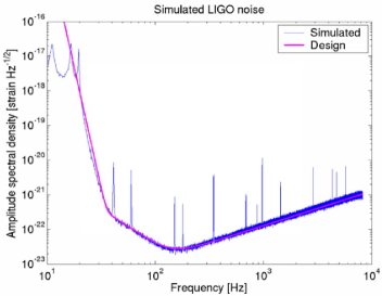
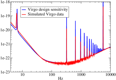
Figure 1: Amplitude spectral density of simulated noise matching the design sensitivity of LIGO (left) and Virgo (right), in strain $/\sqrt{Hz}$.

In addition to the detector noise, each group provided a series of non-coincident, optimally oriented, neutron star inspiral waveforms to be injected in the data. The events were generated using second order post Newtonian waveforms.

A number of 26 such events were randomly injected in the LIGO data, with source masses either $[1.4M_{\odot},1.4M_{\odot}]$ or $[1M_{\odot},2M_{\odot}]$, with $M_{\odot}$ the mass of the Sun. The source was assumed to be located at a distance either 20, 25, 30 or 35 Mpc from the detector. The waveforms were generated with a starting frequency of 40 Hz, consistent with the interferometer sensitivity, and injected with an average period of about 400 seconds.

In the Virgo data, 11 inspiral events with source masses $[1.4M_{\odot},1.4M_{\odot}]$ were randomly injected with an average period of about 900 seconds. The starting frequency of the waveform was 24 Hz, and the events were injected with a signal to noise ration (SNR) of 10, corresponding to a distance of 24.8 Mpc between the source and the detector.

All data were stored in frame format, and only calibrated strain data were exchanged. Details of the injected signals were also exchanged in advance.

2 Analysis Pipelines

Each group analyzed both sets of LIGO and Virgo simulated data, using their own analysis pipeline. In this section we give a short description of the analysis codes used. They are all based on matched filtering implemented on a bank of templates covering some given space for the source masses.

2.1 LSC Pipeline

A detailed description of the LSC inspiral search pipeline can be found in [3]. We only summarize here the main features of the algorithm.

The data set is split into analysis chunks of 15 overlapping segments. The length of each segment is chosen so as to be at least four times the duration of the longest template in the bank, which depends on the starting frequency of the search. For each analysis chunk, a bank of templates is created, generating templates in the frequency domain using second order post Newtonian waveforms.

The data are filtered with each template in the bank, and a trigger is recorded each time the maximum of the SNR of a filter output exceeds some threshold. Maxima above threshold separated in time by less than the length of the template are considered the same trigger, but triggers from different templates are recorded individually.

2.2 Virgo Pipeline

For this project, the multi-band search (MBTA) [4], which is one of the template-based analyzes implemented by the Virgo Collaboration, has been used. In this approach, the templates are split for efficiency into low and high frequency parts and then combined together, in a hierarchical way.

For each frequency band, a bank of “real” templates is created, generating templates first in the time domain using second order post Newtonian waveforms. These templates are called real because they are actually used to filter the data. The analysis is done on data segments long enough to accommodate at least twice the longest template length.

On the full frequency band, a bank of “virtual” templates is created with the same criteria, but the templates are not used directly in matched filters. For each virtual template, the output of the corresponding filter is built coherently from the outputs of the filters based on the real templates associated to the virtual template in each frequency band.

A trigger is recorded each time the maximum of the SNR of a (virtual) filter output exceeds some threshold. The triggers are then clustered both in time and over the template bank; triggers issued by different templates but with matching ending time are considered the same event.

A ”flat search” more similar to the LSC pipeline has also been implemented in Virgo, and was run on both data sets. The triggers obtained are consistent with those resulting by the MBTA analysis and for the sake of article’s clarity we do not report further details. Readers interested in the ”flat search” approach can refer to the paper by L.Bosi et al. in these proceedings [5].

3 Production of Trigger Lists

The LSC pipeline and the MBTA pipeline were used to analyze both data sets, with common search parameters agreed upon beforehand by the two groups. The parameters of the analysis are summarized in table 1. The source mass space explored was 1-3 M_⊙. The template banks were generated matching a grid in the mass space created with a minimal match criterion of 95%, ensuring that no event in that mass space should be detected with a SNR loss greater than 5%.

The starting frequency $f_{low}$ used to build the templates was set to different values to analyze the LIGO data and the Virgo data, to be consistent with the SNR accumulation driven by the sensitivity curves of both experiments; $f_{low}$ was set to 40 Hz for LIGO data and to 30 Hz for Virgo data. In addition, the MBTA code was run with a splitting frequency between the low and high frequency bands chosen so as to share in an approximately equal way the SNR between the two bands (see table 2). Triggers were recorded when the SNR exceeded a threshold of 6.

	LIGO data	Virgo data
Mass range	1-3 M⊙	1-3 M⊙
Grid minimal match	95%	95%
Starting frequency $f_{low}$	40 Hz	30 Hz
Longest template duration	$\sim$ 45 seconds	$\sim$ 96 seconds
SNR threshold	6	6

Table 1: Common search parameters for the LSC and MBTA pipelines.

The layout of the template banks depends on the noise power spectral density of the instrument, and on the value chosen for $f_{low}$. The way the LSC designs the grid used to place the templates is described in [6]. The Virgo group creates the grid according to a 2D contour reconstruction technique based on the parameter space metric [7]. The two methods lead to numbers of templates that differ by about 40%, as is reported in table 2.

	LSC pipeline	MBTA pipeline	LSC pipeline	MBTA pipeline
	on LIGO data	on LIGO data	on Virgo data	on Virgo data
Number of templates	$\sim$ 3500	$\sim$ 1900	$\sim$ 9500	$\sim$ 6100
Band splitting frequency	not relevant	130 Hz	not relevant	95.3 Hz
Number of jobs	6	1	3	7
Type of processor	1 GHz Pentium II	Xeon 2 GHz	Xeon 2.66 GHz	2.4 GHz Pentium IV
Total memory		0.9 GByte		4.5 GBytes
Total processing time	$\sim$ 46 hours	$\sim$ 13 hours	$\sim$ 88 hours	$\sim$ 28 hours
$\frac{{\rm processing\ time}\times{\rm processor\ speed}}{{\rm number\ of\ templates}}$	$\sim$ 47 s GHz	$\sim$ 49 s GHz	$\sim$ 89 s GHz	$\sim$ 40 s GHz

Table 2: Configuration and computing cost of each analysis.

Table 2 also provides information about the way the production was done for the two pipelines and each data set: on how many jobs the production was split (the LSC pipeline analyzes different time periods in different jobs, whereas the MBTA explores different regions of the parameter space), which type of processor was used and how much resources were needed (memory, total processing time after initialization).

In order to compare the performances of the two pipelines, the table also quotes the amount of time required to analyze one template, normalized by the speed of the processor. The speeds of all the analyses are about the same, apart from the LSC pipeline running on Virgo data, presumably because it did not use a number of points which was a power of 2, and this would have slowed down the fast Fourier transforms. Regarding the MBTA pipeline, the version of the code used was optimized for memory.

4 Comparison of Triggers

Since both groups use different formats to record their triggers, some specific software was developed to convert triggers from one format to the other.

4.1 Injection Identifications

The first point was to compare how both groups’ detection procedures were able to identify the inspiral injections present in the data streams. In each trigger list, an element is tagged true if the ending time of the event matches the ending time of the injected event within $\pm$ 20 ms. The detection efficiency and the identification overlap of the two pipelines are very good: The 11 events injected in the Virgo data are detected by both pipelines. In the LIGO data stream, there is one event out of 26 which is missed by both analyzes, and one event which is identified by the LSC pipeline but missed by the Virgo pipeline. This is interpreted as a threshold effect since both events were injected at a distance of 35 Mpc, leading to an expected low value of 6.40 for the SNR.

An issue was to associate the triggers produced by the LSC pipeline with those produced by MBTA. The LSC triggers are not clustered over the template bank, so that many of them usually correspond to a given injection. On the other hand, MBTA usually produces a single trigger per injection due to the clustering over templates. This becomes important to further compare the detection parameters of events identified by the codes of the two groups. For each injection, the trigger with highest SNR among the LSC associated triggers was kept to be compared to the corresponding MBTA trigger.

4.2 Signal to Noise Ratio

For each injected event coincidentally detected by both pipelines, the measured signal to noise ratio was compared. The result of the comparison is shown in figure 2. On both data sets, there is a good correlation and general agreement between the SNRs measured by the LSC and MBTA pipelines.

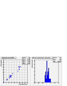
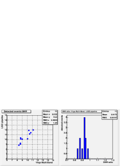
Figure 2: Comparison of the measured signal to noise ratio. The top row corresponds to the LIGO produced data, while the bottom row is Virgo produced.

In the case of the Virgo data, the two pipelines appear to be slightly biased in opposite directions, so that there is an average 8% discrepancy between the measured SNRs. The statistically significant part of the difference can be attributed to differences in the way the template grids are generated. In particular, while the LSC grid has a point very close to $[1.4M_{\odot},1.4M_{\odot}]$, the grid used by MBTA does not have a template very close to this point where signals were injected. The closest template has a match only slightly above the 95% required minimal match.

4.3 Distance

The distances to the source measured by both pipelines were also compared, as shown in figure 3. As expected, the same correlation and general agreement as in the SNR case is observed. The quality of the agreement is somewhat degraded, however, and in the worst case of the Virgo data, is at the 12% level.

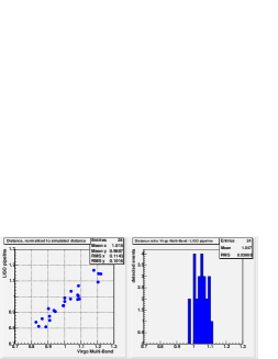
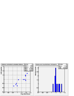
Figure 3: Comparison of the measured source distance, normalized to the simulated distance. The top row corresponds to the LIGO produced data, while the bottom row is Virgo produced.

The systematic effects at the origin of this bias in the distance recovery are yet to be investigated. In the MBTA case, for instance, it is clear that the distance overestimation exceeds the loss in the measured SNR, which is not consistent. The way triggers from the two pipelines are associated for comparison could also have an impact.

4.4 Arrival Time

A crucial parameter in view of coincident analysis is the arrival time of the detected events. It is essential that the two pipelines agree on this parameter. Figure 4 shows a comparison of the arrival times quoted by the LSC and MBTA pipelines.

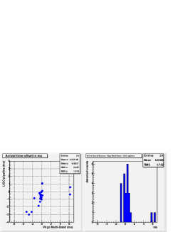
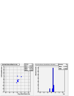
Figure 4: Comparison of the measured arrival time. The top row corresponds to the LIGO produced data, while the bottom row is Virgo produced.

Interestingly, the plots exhibit some correlation also for the arrival time. In the case of LIGO data, the MBTA pipeline is clearly off for two events detected by the same template which does not behave well as far as the arrival time is concerned. Apart from these two events, which are detected with a low SNR, the agreement between the measured arrival times is at the 1 ms level.

4.5 Source Mass

The last test was to see how accurately the mass parameters of an injected inspiral signal could be reconstructed. Figure 5 shows that neither pipeline is able to obtain the component masses particularly accurately. On the other hand, a reliable estimate of the chirp mass, $m_{chirp}=(m_{1}m_{2})^{3/5}/(m_{1}+m_{2})^{1/5}$, can be obtained. For the two data sets, we see that the accuracies of both pipelines are comparable. Furthermore we recover the chirp mass very well - errors less than $4\cdot 10^{-3}$ in LIGO data and $1\cdot 10^{-3}$ in Virgo data (in contrast to previous sections, the two numbers we quote here are based on the different data sets rather than the different pipelines, which actually give comparable results). Thus, the chirp mass seems a natural parameter to use in coincidence tests. The better accuracy in Virgo data is due to better low frequency sensitivity and hence longer waveforms. The errors in the chirp mass appear uncorrelated between the pipelines, and are probably due to the specific template placement algorithms used.

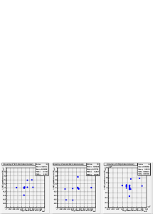
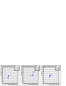
Figure 5: Comparison of the measured source mass parameters. The top row corresponds to the LIGO produced data, while the bottom row is Virgo produced.

As a post-processing on selected data sections, a Bayesian parameter estimation routine was also applied to the sections of data where the inspiral triggers were found. A Markov chain Monte Carlo (MCMC) routine using a Metropolis-Hastings algorithm generated estimates for the posterior probability distribution functions (PDFs). This method, which is designed to find 2.5 post Newtonian inspiral signals, is described in [8, 9]. Figure 6 shows examples of the MCMC produced posterior PDFs for the chirp mass for two of the signals analyzed. For the LIGO produced signal with $m_{1}$=1 $M_{\odot}$, $m_{2}$ =2 $M_{\odot}$ (chirp mass = 1.2167 $M_{\odot}$) the posterior PDF for the chirp mass overlaps the injected value. For the Virgo produced signal with $m_{1}$=$m_{2}$ = 1.4 $M_{\odot}$ (chirp mass =1.2188 $M_{\odot}$) the mean of the posterior PDF for the chirp mass differs by 0.23% from the injected value. This slight difference, also seen with the LIGO produced signals with $m_{1}$=$m_{2}$=1.4 $M_{\odot}$, is likely due to the different nature of the signals; the generated signals were 2.0 post-Newtonian in the time domain, while the MCMC searches for 2.5 post-Newtonian in the frequency domain. The fact that there is not a complete one to one match between these two signals is reflected in these estimates.

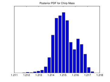
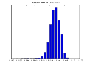
Figure 6: Two examples of posterior PDFs produced by the MCMC for the chirp mass. Left: LIGO produced signal at [1 $M_{\odot}$, 2 $M_{\odot}$] (chirp mass = 1.2167 $M_{\odot}$), PDF mean= 1.2152, RMS = 0.298. Right: Virgo produced signal at [1.4 $M_{\odot}$, 1.4 $M_{\odot}$ (chirp mass =1.2188 $M_{\odot}$), PDF mean=1.2158, RMS = 0.185.

5 Conclusion

In this first project based on simulated data, the LIGO-Virgo joint working group has had the opportunity to run analysis pipelines from the two collaborations on data sets produced by both sides. In doing so, it has been possible to gain better understanding and - most importantly - confidence in each other’s detection procedures, since both analysis pipelines have shown to detect the same events with comparable parameters. This project has thus established the grounds for future work toward collaborative data analysis in the search for inspiral gravitational wave signals.

References

References

- [1] Proposal for joint LIGO-Virgo data analysis, LIGO-T040137-08-Z and VIRGO-PLA-DIR-1000-201 (2004)
- [2] M.Zanolin et al., Joint LIGO/Virgo working group (these proceedings)
- [3] LIGO Scientific Collaboration, B.Abbott et al., Phys. Rev. D 69 (2004) 122001
- [4] Virgo Collaboration, F.Marion et al., Proceedings of the Rencontres de Moriond 2003, Gravitational Waves and Experimental Gravity (2004)
- [5] Virgo Collaboration, L.Bosi et al. (these proceedings)
- [6] B.J.Owen and B.S.Sathyaprakash, Phys. Rev. D 60, 022002 (1999)
- [7] D.Buskulic et al, Class. Quant. Grav. 20 17 (2003) 789
- [8] N. Christensen, R. Meyer and A. Libson. Classical and Quantum Gravity, Vol. 21, pp. 317 (2004)
- [9] N. Christensen and R. Meyer, Physical Review D, Vol. 64, p. 022001 (2001)