Variable placement of templates technique in a 2D parameter space for binary inspiral searches

Abstract

In the search for binary systems inspiral signal in interferometric gravitational waves detectors, one needs the generation and placement of a grid of templates. We present an original technique for the placement in the associated parameter space, that makes use of the variation of size of the isomatch ellipses in order to reduce the number of templates necessary to cover the parameter space. This technique avoids the potentially expensive computation of the metric at every point, at the cost of having a small number of “holes” in the coverage, representing a few percent of the surface of the parameter space, where the match is slightly lower than specified. A study of the covering efficiency, as well as a comparison with a very simple regular tiling using a single ellipse is made. Simulations show an improvement varying between 6% and 30% for the computing cost in this comparison.

1 Introduction

In searching for gravitational wave signals from coalescing binary compact objects, one commonly uses an optimal filtering technique [1]. This technique consists of the comparison of the output signal of an interferometric gravitational waves detector with a family of expected theoretical waveforms, called templates. Each template depends on one or more parameters $\left\{\lambda_{i}\right\}$. The choice of the templates in the $\left\{\lambda_{i}\right\}$ parameter space, called placement, is the purpose of this paper. We restrict ourselves to a 2D parameter space, considering spinless templates computed at second post-newtonian order.

We will first describe in section 2 the motivations of our placement technique, comparing it with a simple uniform paving of the parameter space. Section 3 describes the calculation of the parameters of the parameter space portion covered by a single template. This portion is in our case well approximated by an ellipse. Next, section 4 treats the triangulation of the parameter space, a step needed by the placement, which is covered by section 5. Finally, performance tests are covered by section 6, where some real use-cases are considered in the context of the Virgo detector [2].

2 Motivations

2.1 Portion of the parameter space covered by one template

The comparison of a signal with one template is made through a Wiener filter [3]:

$$\langle\tilde{a},\widetilde{T}\rangle=2\left[\int^{f_{s}}_{f_{i}}\frac{\tilde{a}(f).\widetilde{T}^{*}(f)}{S(f)}\textrm{d}f+\textrm{c.c.}\right]$$ (1)

This is essentially a weighted intercorrelation, $\tilde{a}(f)$ being the interferometer output and $\widetilde{T}(f)$ the template. $S(f)$ is the noise power spectral density (PSD) of the detector, $f_{i}$ and $f_{s}$ are the lower and upper limits of the detector spectral window.

Each template is represented by a point in a multidimensional parameter space. After taking care of most extrinsic parameters (like time of arrival or initial orbital phase of the system) by maximizing the output of the optimal filter over them [5], there remain only two parameters, that we will call $\lambda_{1}$ and $\lambda_{2}$. Those parameters may be the masses of the two bodies but in general, one uses parameters derived from the masses that simplify the calculations.

A template corresponding to parameters $(\lambda_{1},\lambda_{2})$ is sensitive to a signal corresponding to nearby parameters $(\lambda_{1}+\delta\lambda_{1},\lambda_{2}+\delta\lambda_{2})$. The difference leads to a decrease in signal over noise ratio (SNR) with respect to the SNR obtained with a signal corresponding to the exact template. For an acceptable loss in SNR, each template covers a portion of the two dimensional parameter space. Following Owen [1] in a geometrical interpretation of the optimal filtering, one is able to define a distance between two templates as the ambiguity function maximized over extrinsic parameters, called “match”. When filtering a signal which has the same shape as a template of parameters $(\lambda_{1}+\delta\lambda_{1},\lambda_{2}+\delta\lambda_{2})$ with a reference template of parameters $(\lambda_{1},\lambda_{2})$, the match is the fraction of the optimal SNR obtained when filtering the reference template with a signal identical in shape to itself.

Given a minimal match $MM$, we can define the region of parameter space around a given point corresponding to a template $T$, the match of which, computed with any template corresponding to a point in the region, will be above $MM$. We will call the boundary of this region the “isomatch contour”. The shape of this boundary may be complex, so one generally uses parameters for which it has been shown that, for high values of the minimal match, ($MM>0.97$) the contour is closed and well approximated by an ellipse [1]. Throughout this paper,instead of masses, we will use chirp times $\tau_{0}$ and $\tau_{1.5}$[4] defined as:

$$\tau_{0}=\frac{5M}{256\eta(\pi Mf_{0})^{8/3}}\qquad\tau_{1.5}=\frac{\pi M}{8\eta(\pi Mf_{0})^{5/3}}$$ (2)

in geometrized units ($G=c=1$), where $M$ is the total mass of the binary system, $\eta=m_{1}m_{2}/M^{2}$ is the symmetric mass ratio and $f_{0}$ a fiducial frequency chosen as the lower frequency cutoff of the detector sensitivity. Results are properly scaled to restore physical units.

The calculation of the parameters of the ellipse may be done analytically for a given spectral density [1][6].

The final goal of our study is to pave the parameter space with isomatch contours in as optimal a way as possible. This is equivalent to finding the minimal set of templates whose isomatch contours pave all the parameter space, without letting any hole or unpaved region [7].

2.2 Simple paving of the parameter space

One simple solution, already described elsewhere, is to calculate the ellipse parameters for the point in the parameter space where it is known to be the smallest and pave the space with this single ellipse [1], obtaining a regular tiling of the parameter space. This is not very different from paving a bidimensional space with circles. As was already noted [7], because of the rotational symmetry, the centers of the circles should sit at the vertices of regular polygons which make a regular tiling of the plane. This is only possible for triangles, squares or hexagons. In the first case, the centers of the circles are placed on the corners of an equilateral triangle, as shown in figure 1 A). It is desirable to have the sparsest possible circles, which means that three circles touch at one single point $P$. The surface region consisting of the points whose closest circle center is $C$ is shown in gray. This is also the surface covered on average by one circle.

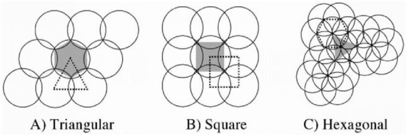
Figure 1: Paving of a plane with different elementary cells. The relevant Voronoi sets are shown in gray.

In the triangular case, it is a hexagon. The set of points which belongs to this region is called the Voronoi set of $C$. As illustrated in figure 1, in the case of a square tiling, the Voronoi set has a square shape and in the case of a hexagonal tiling, the Voronoi set has a triangular shape. It has been shown [7], as one would intuitively expect, that the most efficient tiling in the case of placement of circles is the triangular one. Of course, in our case, the circles are skewed according to the parameters of the initially calculated ellipse.

The tiling is extended outside the parameter space to make the coverage complete. The ellipses, the center of which lies in a physically forbidden region (under the equal mass line), are shifted towards the allowed region, staying on the equal mass line, still ensuring the completeness of the coverage. An example is given in fig. 2, where the ellipse at the extreme right (smallest masses) represents the only computed point.

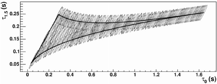
Figure 2: Example of a regular tiling of a parameter space. The templates are computed at 2 PN order in the mass range [5;50] $\textrm{M}_{\odot}$, the minimal match being 0.95, the frequency range [50;2000] Hz with the Virgo PSD.

2.3 Improvements to this method

The above simple method is very fast but, assuming that one uses the smallest possible ellipse, is clearly suboptimal in most cases. It gives a higher number of templates than would be ideally needed if one was able to calculate the shape of the isomatch contours at any given point of the parameter space and use those bigger shapes to cover the space. A second problem would then arise, since an optimal tiling of the parameter space with varying shapes is far from being obvious. The principle of reconstruction of exact isomatch contours has been described previously [9] as well as a preliminary placement method.

We present in this paper an extension and improvement of this method in the case where the elliptic approximation for isomatch contours is assumed valid.

3 Computation of ellipse parameters

Before doing the placement, one should be able to calculate as fast as possible the ellipse parameters at any given point in the parameter space. This is done by

• Calculating the ellipses at a chosen set of points (we obtain “seed ellipses”).

• Triangulating the parameter space with this set. Actually, as we will see, those two steps are closely linked. We give in appendix a short tutorial about triangulation and computational geometry.

• Interpolate linearly ellipses at any point using the previously calculated seed ellipses. This step is much faster than an analytical computation.

3.1 Computation of seed ellipses

The seed ellipses are computed using the algorithm included inside the LIGO Analysis Library (LAL) [13]. This algorithm uses the procedure described in [8]. The metric components used to find the parameters of the ellipse are calculated using the moments of the PSD curve.

3.2 Triangulation and interpolation

The triangulation of the parameter space deserves hereafter a section by itself. Once it is computed, each point $P$ in the parameter space belongs to one and only one triangle whose corners are three seed points. One is able to interpolate linearly the shapes (resp. metric parameters) of the three seed ellipses to obtain the parameters of the ellipse (resp. metric) at point $P$ (see fig. 3).

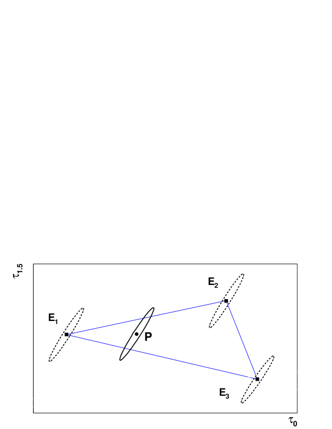
Figure 3: Linear interpolation between analytically calculated ellipses $(E_{1},E_{2},E_{3})$, that may differ in size and orientation, at an arbitrary point P in a triangle.

4 Triangulation of the parameter space

The triangulation of the parameter space is done using standard techniques known in computational geometry. The notions necessary to understand the present study are explained in appendix. The base algorithm used is known as the Bowyer-Watson [14][15] algorithm.

4.1 Triangulation algorithm adapted to the CB parameter space

The Bowyer-Watson algorithm is quite simple but needs adaptation to our problem. We need to take care of the fact that the borders of the parameter space are not convex and we need to choose which points to use for the triangulation.

The main idea of our adapted algorithm is to start from an existing triangle at the corners of which sit three already calculated ellipses $\{E_{1},E_{2},E_{3}\}$ and subdivide it only if necessary, i.e. if for any point $P$ inside the triangle, the ellipse linearly interpolated between $\{E_{1},E_{2},E_{3}\}$ is different enough from the one calculated using the metric at that point. Let $E_{i}$ be the interpolated ellipse and $E_{c}$ the calculated one. $\sigma$ being the measure of the surface of $E_{i}$, $\sigma_{out}$ the surface of $E_{i}$ that does not intersect $E_{c}$ (fig. 4), the variable describing the difference between $E_{i}$ and $E_{c}$ has been chosen as the proportion

$$p=\frac{\sigma_{out}}{\sigma}$$ (3)

It was not deemed necessary to also take into account the surface of $E_{c}$ that does not intersect $E_{i}$, because if $\sigma_{out}$ is null, the interpolated ellipse is completely inscribed inside the calculated one and we are simply going to make a more dense placement at a later stage.

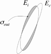
Figure 4: The variable indicating the difference between the two interpolated and calculated ellipses at the same point is the proportion of the surface of the interpolated ellipse not common to both ellipses.

A limit is set on this variable to stop the subdivision of triangles.

4.1.1 Division of an existing triangle

Given an existing triangle, a choice has to be made on the points appropriate for its subdivision. Ideally, one would use the points which have the highest proportion $p$. It is however impractical, and very expensive in terms of computing power to test all the points in a triangle to find the one with the higher $p$. We chose to test only the middle points of each segment forming the triangle.

Each of these three points is inserted and used to subdivide the triangle following a Delaunay method, but considering only the triangle, not the adjacent ones that may exist in the ongoing triangulation process. If the middle point of a segment is outside the parameter space, it is replaced by the closest point on the border, perpendicularly to the segment (fig. 5). Some peculiar situations (two middle segment points outside the parameter space for example) are taken into account. All subtriangles generated outside the parameter space are removed.

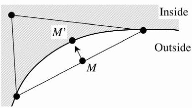
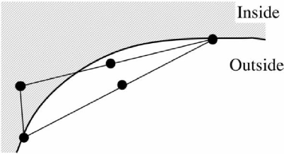
(a)	(b)

Figure 5: Replacement of a point $M$ outside the parameter space by a point $M^{\prime}$ on the border close by (a). A peculiar case, which is taken into account, is also shown (b)

From the description above, it is obvious that the final triangulation will not be strictly speaking a Delaunay one, since we use the Delaunay criterion only locally for a triangle subdivision.

4.1.2 Global algorithm view

We start from the triangle formed in the $(\tau_{0},\tau_{1.5})$ parameter space by the three angular points corresponding to $(m_{min},m_{min})$, $(m_{min},m_{max})$ and $(m_{max},m_{max})$, where $m_{min}$ and $m_{max}$ are respectively the minimal and maximal masses of the binary system members considered.

The triangle is then recursively subdivided as described above. Since there is a limit on the $p$ proportion of each inserted point, the subdivision will stop naturally when the mesh becomes dense enough. These successive refinement steps are illustrated in figure 6. In order to avoid too big a number of calculated ellipses, and to limit the computing time, the number of refinement steps has been arbitrarily limited to 7. It was verified that this doesn’t bring any problems, except in the lower left corner of the parameter space, corresponding to high masses (above 10 $\textrm{M}_{\odot}$) for both objects. In that case, the placement may be somewhat wrong but a posteriori Monte-Carlo tests show an undercoverage not exceeding 2% of the total parameter space surface.

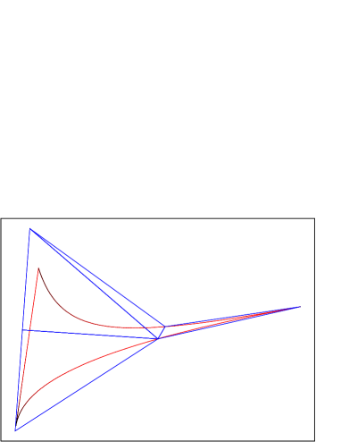
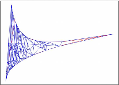
Refinement step 1	Refinement step 5

Figure 6: Mesh refinement steps. Starting from a triangle enclosing the parameter space, insert points and retriangulate while the proportion of discrepancy $p$ between interpolated and calculated ellipse is greater than a limit $p_{lim}$.

As may be noted on figure 6, the tesselation of the parameter space is extended in the physically allowed region to avoid some extrapolation side-effects in the following placement procedure.

4.2 Extrapolation outside border of the parameter space

Each ellipse calculated for the placement procedure described hereafter is actually interpolated inside one of the triangles found during the triangulation step. If the point considered by the placement is outside of the tesselated (triangulated) part, it doesn’t belong to any triangle a priori. We will see that the placement procedure needs to spill over the strict borders of the parameter space to ensure complete coverage, and it may happen that a determination of ellipse parameters is needed outside the tesselated part. Furthermore, the calculation of the metric is impossible in the disallowed (physically forbidden) region under the equal mass line in the $(\tau_{0},\tau_{1.5})$ parameter space. Therefore, we cannot triangulate that region since we cannot calculate true ellipses or contours in it.

Thus, we need to provide a way to extrapolate the ellipse parameters outside the strictly tesselated part of the space. As will be seen later, the final step of the placement procedure consists of shifting the points found in the forbidden region so that they fall in the allowed one. But extrapolation is needed all around the space border during the placement, albeit in a limited area.

For a given point $A$ outside the parameter space, it is natural to associate it with the closest triangle of the tesselation. The word ”closest” should be taken with care, as closest in euclidian distance doesn’t mean more adequate for our purposes. We consider only the triangles which border the tesselated region, i.e. which have one side that is not common to another triangle, thus delimits the border of the tesselation (fig. 7). Once the triangle associated with the point $A$ is determined, one can do a linear extrapolation of the ellipse parameters, as for the points inside the triangle.

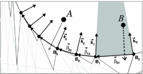
Figure 7: Association between a point outside the triangulated part of the parameter space and a triangle on the border

The choice of the triangle associated with a given point $A$ is done as follows. We define the vectors $\vec{\beta}_{ij}$ which join two successive vertices $B_{i}$ and $B_{j}$ lying on the border of the tesselated part of the parameter space. Each vertex $B_{i}$ is associated with a vector $\vec{k}_{i}$ whose direction is pointing towards the outside of the space and is an average of the normal to two consecutive vectors $\vec{\beta}_{ki}$ and $\vec{\beta}_{ij}$.

A point $A$ will be associated with the triangle containing the vertices $B_{i}$ and $B_{j}$ if it is located in the domain delimited by $\vec{\beta}_{ij}$ and the two lines defined by $(B_{i},\vec{k}_{i})$ and $(B_{j},\vec{k}_{j})$. An example of such a domain is shown in gray in figure 7.

Clearly, the very simple extrapolation we describe is valid only for the points close to the space boundary. The lines $(B_{i},\vec{k}_{i})$ will cross and it is not possible to associate a point and a triangle beyond those crossings. Furthermore, the validity of the extrapolation is not guaranteed for points pushed away from the boundary of the parameter space. In our case, where we marginally extend the calculation of the metric outside the borders, this shows not to be a problem.

4.3 Results in concrete cases

Figure 8 shows triangulation in a few real cases.

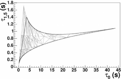
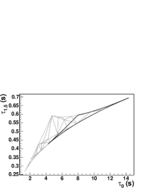
$m_{min}=1\textrm{M}_{\odot}$, $m_{max}=30\textrm{M}_{\odot}$,	$m_{min}=1.95\textrm{M}_{\odot}$, $m_{max}=4.05\textrm{M}_{\odot}$,
$F_{l}=40$ Hz, $F_{h}=2000$ Hz,	$F_{l}=40$ Hz, $F_{h}=2000$ Hz,
$PN=2$, $NStep_{max}=5$, $N_{T}=152$	$PN=2$, $NStep_{final}=4$, $N_{T}=31$

Figure 8: Examples of triangulations representing real use cases for CB searches in Virgo. The black line represents the border of the parameter space. The triangulation area is extended outside to prevent extrapolation problems. See the text for an explanation of computing conditions.

• $m_{min}$ and $m_{max}$ are the minimal and maximal masses of the parameter space

• $F_{l}$ and $F_{h}$ the lower and higher frequency cutoffs used for the generation of templates

• $PN$ is the order of the post-newtonian expansion

• $NStep_{max}$ is the limit imposed on the number of triangulation steps

• $NStep_{final}$ is the number of steps effectively needed to satisfy the surface proportion condition for all the ellipses generated, without reaching the $NStep_{max}$ limit

• $N_{T}$ is the number of calculated points in the triangulation to reach the $NStep_{max}$ or $NStep_{final}$ limit

• The noise spectral density used was a Virgo-like one, shown on fig. 9

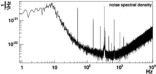
Figure 9: Noise spectral density for the real use cases.

5 Placement

5.1 Isomatch properties

Once the triangulation and seed ellipses have been generated, the placement is done in two stages. Both rely on basic properties of isomatch contours described in [9], namely:

• The match symmetry between two contours. If $\widetilde{T}_{1}$ and $\widetilde{T}_{2}$ are two normalized templates, one has $\langle\widetilde{T}_{1},\widetilde{T}_{2}\rangle=\langle\widetilde{T}_{2},\widetilde{T}_{1}\rangle=M$. Thus, the point in the parameter space corresponding to $\widetilde{T}_{1}$ is located on the isomatch contour of value $M$ corresponding to $\widetilde{T}_{2}$, and conversely, the point corresponding to $\widetilde{T}_{2}$ is located on the isomatch contour of value $M$ corresponding to $\widetilde{T}_{1}$. In practical computations, the match symmetry may not be absolutely verified because in general one maximizes over the initial phase of one template (say $\widetilde{T}_{1}$), which is not done for the signal ($\widetilde{T}_{2}$). This has proven to be negligible for smooth variations of the metric throughout the parameter space, which is roughly the case in our tests using the LAL, except perhaps for high masses, $>10\textrm{ M}_{\odot}$.

• To place an ellipse with respect to another in an optimal way, one introduces a guiding ellipse. This allows to place three ellipse sets (fig. 11). The three ellipses intersect at the center of the guiding ellipse.

In the course of the running of the algorithm, if two of the ellipses are placed, the third one may be positioned naturally on the border of the guiding ellipse by maximizing the surface of the triangle formed by the centers of the three ellipses.

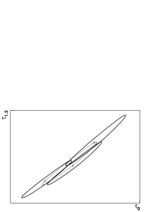
Figure 10: Placement of three contours in the ($\tau_{0}$,$\tau_{1.5}$) plane

Figure 11: First stage of placement along the equal mass line

5.2 First stage

The first stage consists of a side by side placement along the equal mass line starting from the $(m_{max},m_{max})$ point (fig. 11). Unlike in the simple placement case where this was avoided, it is the most efficient way of paving while only one ellipse is needed to cover the parameter space along the direction of the semi-major axis of the ellipse, an almost vertical direction in most of our cases.

The principle is described in figure 12. Starting from an ellipse $E_{i}$ the center of which $C_{i}$ lies on the equal mass line, a choice is made (explained hereafter) of the position $C_{g}$ of the center of a guiding ellipse along the border of $E_{i}$. Because of the isomatch contour properties stated above, $C_{i}$ lies on the guiding ellipse. It is also on the equal mass line. $C_{i+1}$ is the other intersection of the guiding ellipse and the equal mass line.

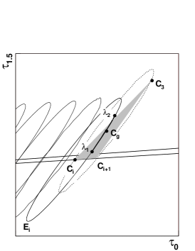
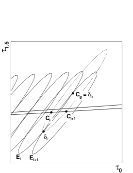
Choice of the position of the guiding ellipse	Position of the next ellipse

Figure 12: principle of the first stage of placement along the equal mass line

The position $C_{g}$ is chosen between $\lambda_{1}$ and $\lambda_{2}$ limits on the $E_{i}$ ellipse, in such a way that the surface of the $\{C_{i},C_{i+1},C_{3}\}$ triangle is maximized. $C_{3}$ is the location of the center of a potential ellipse $E_{3}$ that would form with $E_{i}$ and the next ellipse $E_{i+1}$ a three ellipse set optimally placed (with the placement conditions imposed by the parameter space lower boundary correponding to the equal mass line). The $\lambda_{1}$ and $\lambda_{2}$ limits are chosen empirically and are subject to the influence of numerical errors as well as interpolation/extrapolation errors.

The next ellipse $E_{i+1}$ is then placed at position $C_{i+1}$. $E_{i+1}$ and $E_{i}$ should ideally intersect at two points $\delta_{h}$ and $\delta_{l}$, $\delta_{h}$ being equal to the center of the guiding ellipse $C_{g}$ and $\delta_{l}$ being in the physically forbidden region underneath the equal mass line. Because of the curvature and variation of the metric, it may happen that $E_{i+1}$ and $E_{i}$ do not intersect. In that case, the position $C_{i+1}$ of $E_{i+1}$ is shifted towards $C_{i}$ along the equal mass line until the point $C_{g}$ comes on $E_{i+1}$.

The first stage placement algorithm stops when $\delta_{h}$ falls inside the parameter space, which means that two ellipses are needed to cover the parameter space in the vertical direction.

5.3 Second stage

The second stage of placement consists of the coverage of the parameter space line by line, as was described in [9].

• One starts from a three ellipse set placed optimally at a point $D_{0}$.

• Then place iteratively ellipses using successive guiding ellipses that follow rules defined in section 5.1. The placement is done alternatively on the left and on the right of the line of guiding ellipses, and successively above and below the initial point $D_{0}$.

• One obtains a two-line set crossing the parameter space (fig. 13). Among the external crossings of the generated ellipses of one of the lines (called $\gamma_{1i}$), a point $D_{1}$ is chosen and the process is iterated.

• At each step, only one of the lines is kept, the other being approximately superimposed with a line generated at the previous step (fig. 13).

• The starting point of each two-line set $D_{i}$ for the step $j$ is chosen among the $\gamma_{(j-1)i}$ as the point outside the parameter space and not in the physically forbidden region which is the closest to the border of the parameter space. Other choices have led to the observation of variations in the direction of two successive lines, giving holes in the coverage of the space.

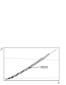
Figure 13: Independent placement of the third line starting from a crossing point on the edge of a first two line set.

The starting point for the first line building of the second stage is the first intersection point $\delta_{h}$ found in the first stage that is inside the parameter space. The placement ends when no ellipse from a line covers any part of the parameter space.

5.4 Correcting points felt outside of the parameter space

Once the first two stages are finished, a cleaning is performed to remove superfluous ellipses that do not cover any part of the parameter space.

It is not possible to do it beforehand because it is not obvious if a given ellipse covers or not a part of the parameter space before it is actually placed. Its center may lie outside of the parameter space but a small part of the ellipse may still cover a portion of the parameter space.

A position correction is also done on ellipses which, while covering a portion of the parameter space, have their center in the physically forbidden region. Those ellipses are shifted following the guiding contour used for their generation until they fall on the equal mass border.

5.5 Examples of computed placements

Figures 14 and 15 show a few real use-cases of placement.

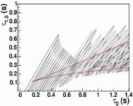
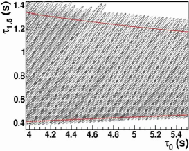
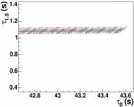
$m_{min}=1\textrm{M}_{\odot}$, $m_{max}=30\textrm{M}_{\odot}$, $MM=0.95$, $F_{l}=40$ Hz, $F_{h}=2000$ Hz,$PN=2$, $N_{T}=152$, $N_{P}=11369$

Figure 14: Example of placement obtained for real world CB searches in Virgo. The black line represents the border of the parameter space. Three portions of space are shown and color of ellipses is varied to help viewing the shapes. See the text for an explanation of computing conditions.

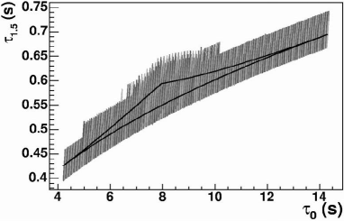
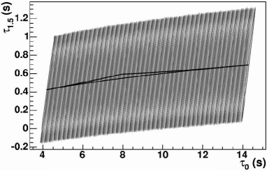
$F_{l}=40$ Hz, $F_{h}=2000$ Hz, $N_{P}=1011$	$F_{l}=40$ Hz, $F_{h}=100$ Hz, $N_{P}=226$
	Only first stage needed to pave all space

$m_{min}=1.95\textrm{M}_{\odot}$, $m_{max}=4.05\textrm{M}_{\odot}$, $MM=0.95$, $PN=2$

Figure 15: Example of placement obtained for real world CB searches in Virgo. The black line represents the border of the parameter space. Color of ellipses is varied to help viewing the shapes. See the text for an explanation of computing conditions.

• $m_{min}$ and $m_{max}$ are the minimal and maximal masses of the parameter space

• $MM$ the minimal match, $F_{l}$ and $F_{h}$ the lower and higher frequency cutoffs used for the generation of templates

• $PN$ is the order of the post-newtonian expansion

• $N_{T}$ is the number of calculated points in the triangulation

• $N_{P}$ is the number of points found in the placement.

• The PSD used was a Virgo-like one (fig. 9)

6 Performance tests

6.1 Number of templates with the simple placement algorithm

The number of templates needed for complete space coverage represents a simple performance estimator. An estimation of this number was already given [8] by computing the ratio between the volume of the parameter space and the proper volume covered by a single template. It was supposed that the packing algorithm used was a square (or hypercubic in $D$ dimensions) one. The proper volume is then, in 2 dimensions

$$\Delta V=2(1-MM)$$ (4)

and in the triangular lattice case (hexagonal Voronoï sets), which was used in our simple algorithm for $D-2$

$$\Delta V=\frac{3\sqrt{3}}{2}(1-MM)$$ (5)

Table 1 shows the numbers we found by using an actual Virgo noise power spectral density. $V_{ps}$ being the volume of the parameter space, $N_{P}^{refSquare}$ is the reference number computed as in [8] assuming a square packing, $N_{P}^{refTriang}$ assumes a triangular packing algorithm and $N_{P}^{simple}$ is the actual number found with our simple algorithm described in paragraph 2.2, which also produces a triangular lattice. Edge effects appear clearly, as the smallest the volume of the parameter space, the largest the difference between $N_{P}^{refTriang}$ and $N_{P}^{simple}$.

$m_{min}\textrm{ (M}_{\odot}\textrm{)}$	$V_{ps}$	$N_{P}^{refSquare}$	$N_{P}^{refTriang}$	$N_{P}^{simple}$
0.5	$1.43\times 10^{4}$	$1.43\times 10^{5}$	$1.10\times 10^{5}$	$1.28\times 10^{5}$
1	$2.57\times 10^{3}$	$2.57\times 10^{4}$	$1.98\times 10^{4}$	$2.59\times 10^{4}$
3	$1.38\times 10^{2}$	$1.38\times 10^{3}$	$1.06\times 10^{3}$	$1.80\times 10^{3}$

Table 1: Comparison of the number of templates obtained with a simple algorithm (triangular packing) and a theoretical number (ratio between parameter space volume and proper volume asuming a square or triangular packing). The minimum mass varies from 0.5 $\textrm{M}_{\odot}$ to 3 $\textrm{M}_{\odot}$. Other conditions : $m_{max}~{}=~{}30\textrm{M}_{\odot}$, $f_{min}~{}=~{}30\textrm{Hz}$, $f_{max}~{}=~{}2000\textrm{Hz}$, $MM~{}=~{}0.95$, Virgo-like PSD.

6.2 Performance gain

With the grid of templates coming out of the new placement algorithm, one can expect a gain in the total computational cost needed to perform a search over the defined parameter space with respect to the simple placement algorithm (paragraph 2.2). This gain is not easily quantified because it depends on the specific search algorithm and on aspects that do not depend on the computational algorithm itself, such as I/O. But it may be estimated in at least two ways:

• firstly, by the gain in the overall number of templates coming out of the placement algorithms (method A).

• secondly, by modeling the “standard” method for doing the optimal filtering and searching for an approximation of the gain (method B).

The optimal filtering technique and an estimation of the computational cost are described by Schutz in [16]. An approximation of the cost (number of floating point operations) for analyzing a set of $N_{tot}$ data values for a given template of length $N_{s}$, and a fractional overlap $x$ of successive data set chunks is:

$$N_{flop}=\frac{N_{tot}}{1-x}[3ln_{2}\frac{N_{f}}{x}+4]$$ (6)

A discussion on the optimal value of $x$ is made in [16], but it does not take into account the I/O costs, as well as exchanges of data between memory and processor, which is found to be critical in our case. Therefore, as explained in [17], we choose $x$ so as to roughly optimize the length and the number of the vectors to be exchanged between the core memory and the CPU. Starting from the expression above and fixing $x=\frac{1}{2}$ for each template, it may be shown that the approximate total number of operations needed to analyze a set of $M$ templates is given by:

$$N_{flop}^{T}=6N_{tot}\sum_{i=1}^{M}[ln_{2}(2f_{s}\tau_{i})+\frac{4}{3}]$$ (7)

where $f_{s}$ is the sampling frequency and $\tau_{i}$ the length of an individual template. This leads to consider a computing performance estimator of the form

$$\xi=\sum_{i=1}^{M}[ln_{2}(2f_{s}\tau_{i})+\frac{4}{3}]$$ (8)

Since we only want an approximate expression, we consider $\tau_{i}=\tau_{0}(i)$, where $\tau_{0}(i)$ is the newtonian chirp time of the coalescing binary producing a given template. We made comparisons between the placement produced by the simple method of paragraph 2.2 and the full placement method. Tables 2, 3 and 4 show the gain on the number of templates and the gain on the performance estimator $\xi$. The conditions of the tests were varied but the base conditions were the following:

• minimal mass $m_{min}=1\textrm{M}_{\odot}$,

• maximal mass $m_{max}=30\textrm{M}_{\odot}$

• minimal frequency for template generation $f_{min}=30\textrm{Hz}$

• maximal frequency for template generation $f_{max}=2000\textrm{Hz}$

• minimal match $MM=0.95$

• power spectral density close to the final Virgo one (fig. 9)

In the tables, $N_{P}^{refSquare}$ is the reference number of templates, computed as in [8] assuming a square packing, as explained above in section 6.1. $N_{P}$ represents the number of templates found by the placement to cover the parameter space, $G_{N_{P}}=(N_{P}^{simple}-N_{P}^{full})/N_{P}^{simple}$ is the gain in the number of templates obtained when going from the simple placement to the full placement method, $N_{T}$ is the number of seed templates necessary to triangulate the parameter space, $G_{\xi}$ is the gain in performance estimator. Unless otherwise noted, the triangulation process was stopped after 7 steps of refinement, which was shown in the section 4.1.2 not to bring problems.

$MM$	$N_{P}^{refSquare}$	$N_{P}^{simple}$	$N_{P}^{full}$	$G_{N_{P}}$	$N_{T}$	$\xi_{simple}$	$\xi_{full}$	$G_{\xi}$
0.90	12840	14047	10746	$23.5\%$	395	$2.46\times 10^{5}$	$1.91\times 10^{5}$	$22.4\%$
0.95	25680	26183	20161	$23.0\%$	381	$4.58\times 10^{5}$	$3.57\times 10^{5}$	$21.9\%$
0.98	64200	61144	47183	$22.8\%$	394	$1.06\times 10^{6}$	$8.34\times 10^{5}$	$21.6\%$

Table 2: Gain on the number of templates and on performance coefficient with respect to a simple algorithm and varying the minimal match. Other conditions: $m_{min}~{}=~{}1\textrm{M}_{\odot}$, $m_{max}~{}=~{}30\textrm{M}_{\odot}$, $f_{min}~{}=~{}30\textrm{Hz}$, $f_{max}~{}=~{}2000\textrm{Hz}$, Virgo-like PSD.

In table 2, the minimal match was varied from $MM=0.90$ to $MM=0.98$, keeping the other parameters equal. As can be seen, an average performance gain of roughly 22% is achieved. It may be noted that the number of templates may also be used as a performance estimator, giving numbers very similar to $\xi$.

$m_{min}\textrm{ (M}_{\odot}\textrm{)}$	$N_{P}^{simple}$	$N_{P}^{full}$	$G_{N_{P}}$	$N_{T}$	$\xi_{simple}$	$\xi_{full}$	$G_{\xi}$
0.5	129507	113531	$12.3\%$	335	$1.28\times 10^{6}$	$1.13\times 10^{6}$	$11.9\%$
1	26183	20161	$23.0\%$	381	$4.58\times 10^{5}$	$3.57\times 10^{5}$	$21.9\%$
3	1829	1106	$39.5\%$	416	$1.65\times 10^{4}$	$1.01\times 10^{4}$	$38.7\%$

Table 3: Gain on the number of templates and on performance coefficient with respect to a simple algorithm. The minimum mass varies from 0.5 $\textrm{M}_{\odot}$ to 3 $\textrm{M}_{\odot}$. Other conditions: $m_{max}~{}=~{}30\textrm{M}_{\odot}$, $f_{min}~{}=~{}30\textrm{Hz}$, $f_{max}~{}=~{}2000\textrm{Hz}$, $MM~{}=~{}0.95$, Virgo-like PSD.

In table 3, only the minimal mass of the stars, hence the size of the parameter space, was varied from $m_{min}=0.5\textrm{M}_{\odot}$ to $m_{min}=3\textrm{M}_{\odot}$. The gain is naively expected to increase with the size of the parameter space. The bigger the parameter space, the higher the variation of metric, hence the bigger the variation in size of the ellipses. The results shown in table 3 vary in the opposite direction. This is explained by edge effects, where the influence of ellipses covering a small part of the parameter space, on or outside the border, and the way they are placed, play a dominant role.

$f_{min}-f_{max}\textrm{ (Hz)}$	$N_{P}^{simple}$	$N_{P}^{full}$	$G_{N_{P}}$	$N_{T}$	$\xi_{simple}$	$\xi_{full}$	$G_{\xi}$
30-100	2191	1948	$11.1\%$	90	$4.09\times 10^{4}$	$1.37\times 10^{4}$	$11.2\%$
100-2000	986	833	$15.5\%$	167	$1.37\times 10^{3}$	$1.17\times 10^{3}$	$15.2\%$
30-2000	12641	11820	$6.6\%$	61	$2.33\times 10^{5}$	$2.18\times 10^{5}$	$6.5\%$

Table 4: Gain on the number of templates and on performance coefficient with respect to a simple algorithm. Two limited frequency ranges are tested: $[30;100]$ Hz and $[100;2000]$ Hz. The mass range is $[1;5]\ \textrm{M}_{\odot}$. Other conditions: $MM~{}=~{}0.95$, Virgo-like PSD.

Finally, table 4 shows the results for a variation in the frequency range. The mass range was limited to $[1;5]\ \textrm{M}_{\odot}$ because for high masses we are reaching the limits of the numerical relevance of the metric calculation.

It may be noted that in practical algorithms, templates will be grouped by groups of similar length. The expression of $\xi$ (equation 8) will take a linear form as a function of the number of templates. This should bring the gains we obtained for the performance estimator closer to the ones obtained with the number of templates.

6.3 Coverage tests

The metric calculation is approximate, especially in the high mass region, where there is yet no good model of coalescence. It is therefore important to do independent tests on the covering efficiency. Monte-Carlo tests were performed by testing randomly scattered points over the parameter space. The distribution of position is uniform in $(\tau_{0},\tau_{1.5})$ parameters. For each point, the corresponding waveform is computed and the match with the templates of the bank is calculated, retaining the highest. Actually, only the subset of templates which are closer than a given distance to the point, in the metric sense, are considered.

The chosen conditions in terms of masses, frequencies and minimal match are the standard ones described in 6.2. Figure 16.A shows the distribution of test points over the parameter space, while figure 16.B shows the distribution of points the match of which is lower than the specified match (0.95 in our case).

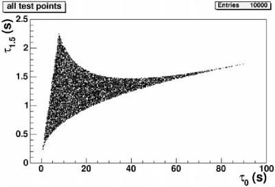
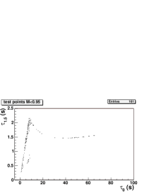
A	B

Figure 16: Monte-Carlo distribution of points in coverage tests. A: all the points, B: points with match $M<0.95$ with the closest template. The conditions are the standard ones.

The low match points (with match $M<0.95$) represent 1.6% of all the test points. There are two possible reasons for the presence of these points. The first is the presence of holes in between ellipses, due to suboptimal placement, the second is a possible miscalculation of the metric in some peculiar cases, for example for high mass binaries. Finer Monte-Carlo tests were performed in small regions relevant for the two cases, and low match point positions were superimposed with isomatch ellipses. The first case is illustrated with figure 17 where it is clearly seen that most of the low match points fall in existing holes of the placement.

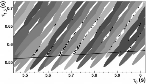
Figure 17: Superposition of a small part of calculated isomatch ellipses in placement and test points with match $M<0.95$. The test points clearly fall in holes formed by locally incorrect placement.

The second case is illustrated in figure 19. The test is made with points chosen in the region $\tau_{0}\in[6.8;7.1]$ and $\tau_{1.5}\in[1.7;2]$ (region named $\sigma_{HM}$), the points being inside the parameter space. It is clear from the picture that all the points of $\sigma_{HM}$ fall well inside an existing ellipse, hence they should have had match $M>0.95$ if the metric was correctly calculated. This situation is explained by the miscalculation of the ellipse orientation, as is illustrated in figure 19. In this figure, the points with $M>0.99$ were considered, and they form a figure clearly showing the wrong orientation of the computed ellipses (several colors depending on the value of the match were used, the darker the points the higher the match).

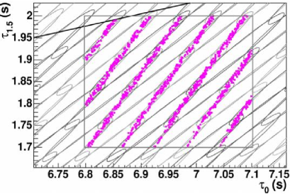
Figure 18: Superposition of a small part of calculated isomatch ellipses in placement and test points with match $M<0.95$. The gray box surrounds the test region.

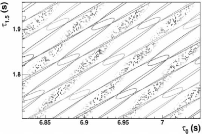
Figure 19: Superposition of a small part of calculated isomatch ellipses in placement and test points with match $M>0.99$. This illustrates the wrongly calculated orientation of the ellipses, leading to a wrong placement.

Figure 21 compares the distribution of the test points match for the full placement algorithm and for the simple placement algorithm. The simple placement is clearly suboptimal, but ensures a complete covering of the parameter space while the optimality is better for the full algorithm, though it does not cover perfectly the parameter space, at the level of a few percent undercoverage. Figure 21 illustrates the influence of miscalculation of the metric. Superimposed to the distribution of the match in the full placement case, is the distribution of the match for $\sigma_{HM}$. This distribution was scaled down proportionately to the surface of $\sigma_{HM}$ region versus the surface of the parameter space to show its contribution to the overall distribution.

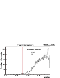
Figure 20: Comparison of the match distribution for the simple and full placement. The red vertical line shows the requested minimal match, 0.95 in this case.

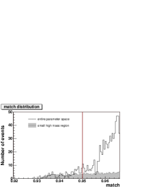
Figure 21: Estimation of the contribution of points in a region where ellipses correspond to high mass with miscalculated metric. The red vertical line shows the requested minimal match, 0.95 in this case.

In general, the two effects, miscalculation and misplacement, are both present with various strength throughout the whole parameter space. Miscalculation is due to wrong approximation of the metric and/or approximations in the triangulation and interpolation steps of the placement algorithm.

In figure 16.B, a clear accumulation of low match points seems to occur in the high mass region. To confirm this, a test was made with a mass range $[m_{min};m_{max}]=[1;10]\textrm{M}_{\odot}$. The match distribution for this test, superimposed on the match distribution of the entire parameter space ($[m_{min};m_{max}]=[1;30]\textrm{M}_{\odot}$) and on the match distribution of $\sigma_{HM}$, is shown in figure 22. It is clear from this figure that the main source of low match points is the miscalculation of the metric for high masses.

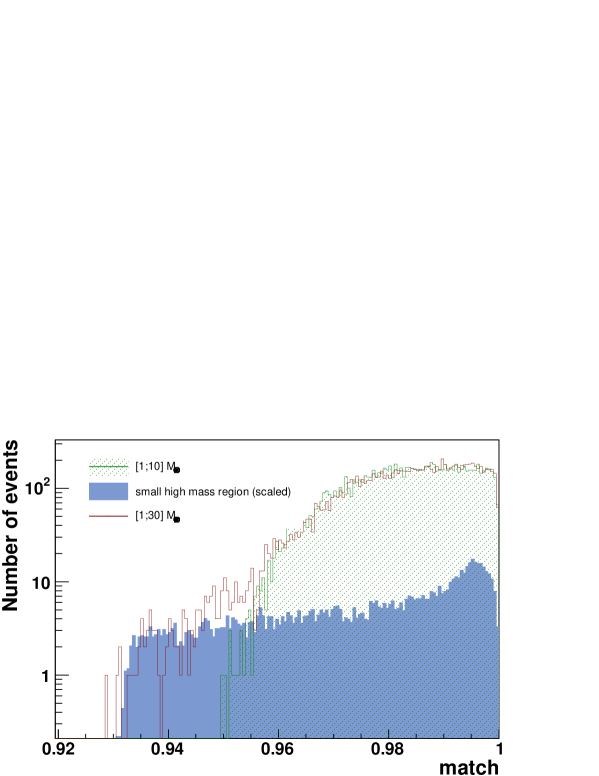
Figure 22: Comparison of match distributions for $[m_{min};m_{max}]=[1;30]\textrm{M}_{\odot}$ and $[m_{min};m_{max}]=[1;10]\textrm{M}_{\odot}$. Also included is the distribution corresponding to a specifically high mass region in the parameter space, scaled proportionately to its surface with respect to that of the whole parameter space.

In order to get an idea of how to easily overcome these problems, one can calculate the proportion of bad match test points as a function of a varying minimal match value $\mathpzc{M}$, for a given placement. This corresponds to enlarging the ellipses obtained with a placement with an initial minimal match $\mathpzc{M}_{0}$. Figure 23 shows the variation of the proportion $\rho$ of test points with match lower than $\mathpzc{M}$ versus $\mathpzc{M}$. From this figure, given a desired bad match points proportion, one gets an estimation of the effective minimal match reached.

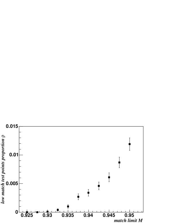
Figure 23: Proportion of bad match test points as a function of an effective minimal match value for a given placement. Only statistical errors are reported.

A question may be raised about the robustness of the algorithm, i.e. is the algorithm adequate for real, noisy data. It is very difficult to assess an “absolute” robustness of the algorithm, because of three main points :

• the difference between the true contour and the calculated ellipse, especially for low matches, which may in some circumstances push the algorithm to its limits.

• the fact that the algorithm is not robust in the case of large and fast variations of the metric.

• the difference between calculated and interpolated ellipses that may, though not in large proportions, affect the algorithm.

There is a need for tools that run online and verify the relevance of the computed grid banks. In the case of problems, it is always possible to switch to the simple algorithm.

6.4 Speed tests and recomputation of the placement

All the tests were performed on a Linux 2.4 GHz Pentium IV workstation and we present in table 5 the computation time in seconds needed for each placement, in increasing number of generated grid points. The time is divided in two, corresponding to the two main steps of the algorithm, namely first the triangulation and generation of seed contours and second the placement itself. There is a rough proportionality between the number of final grid points and the time, with a quasi constant term corresponding to the first step (the number of generated seed contours being always of the same order of magnitude).

$m_{min}-m_{max}\textrm{ (M}_{\odot}\textrm{)}$	$MM$	$N_{T}$	$N_{P}^{full}$	Time (s)
3-30	0.90	418	643	60
3-30	0.95	416	1106	67
3-30	0.98	402	2362	84
1-30	0.90	395	10746	203
1-30	0.95	381	20161	294
1-30	0.98	394	47183	575
0.5-30	0.90	335	59103	742
0.5-30	0.95	346	113531	1287

Table 5: Computation time for different placements on a 2.4 GHz Pentium IV Linux workstation.

The frequency of recomputation of the placement is still under consideration in Virgo. It depends on the change rate of the shape of the sensitivity curve over time, the stability of which is not yet fully assessed for future science runs. The numbers given in table 5 may seem too large for a frequent recomputation, for instance every 15 minutes, in the case of large volume parameter spaces. Though such a frequency is not expected for the final Virgo science runs, we may need to consider a parallelization of the algorithm. The part of the algorithm that could be parallelized efficiently is the placement part, but one should not expect more than an estimated factor 2 to 5 improvement in overall computing time, due to the sequential nature of the algorithm. Indeed, in one line of ellipses, ellipse number $n$ may not be placed before ellipse number $n-1$. Only the placement of complete lines may be somewhat decorrelated.

7 Comparison with previous studies and perspectives

Beside very important pioneering efforts [1][8] the results of which are now widely used, several previous studies were done for the template placement problem. We believe that our method is somewhat complementary to them. For example, the placement algorithm used in [18] for extended hierarchical searches is based on a square tiling. This is justified in this case by the low minimal match value used ($\Gamma=0.8$), which gives very irregularly shaped contours. Our method could probably be adapted to such a case by applying methods such as in [9] to determine the shape of the contours, but an important effort has to be made to improve the speed of the shape reconstruction algorithm, which is going to be one of the main limiting factors.

Another example is the paper of Arnaud et al.[19] where authors devise a 2D tiling method and test it in the case of supernova ringdown signals. It is very difficult to make a direct comparison between this algorithm and ours. The very large parameter space curvature described by Arnaud et al is likely to bring some holes if we apply directly our tiling method to ringdown signals. This would imply the need for an improvement to our placement procedure. On the other hand, the Arnaud 2D tiling method was not yet applied to the case of a $(\tau_{0},\tau_{1.5})$ inspiral parameter space and it is not clear what would be the result in terms of speed and possible overcoverage.

The computational geometry tools that we used are still valid in higher dimensional spaces. It may be tempting to consider the extension of our algorithm to multidimensional searches. In that case, the main challenge would be to improve the algorithm speed, since the number of contours in nD is roughly going as

$$N_{n}\approx N_{2}^{\frac{n}{2}}$$ (9)

Where $N_{2}$ is the number of contours obtained in 2D. This is of course a “worst case” scenario where the granularity is the same (and high) in all dimensions.

8 Conclusion

We presented a technique for doing the placement of isomatch ellipses on a template parameter space using triangulation and interpolation of seed ellipses. A comparison is done with a simple regular triangular tiling using a single ellipse. This comparison shows an improvement between 6% and 30% depending on the mass range and frequency range. Some coverage tests were also performed that show a few percent undercoverage of the parameter space, mainly in the high mass region. This undercoverage seems to come from the miscalculation of the metric for high masses. Finally, speed tests were made.

9 Acknowledgements

We would like to thank all our Virgo colleagues from the inspiral data analysis group, and particularly Andrea Viceré for his help in bringing an important piece of Mathematica code and insightful comments. We would also like to acknowledge the use of the Ligo Analysis Library, and thank Thomas Cokelaer for his precious help.

References

Appendix: A few notions of computational geometry

Since computational geometry is not very commonly used in our field, we will give a very short introduction to the notions useful for the present study. It is in no way exhaustive or pretending to be accurate. More details may be found in [10] or [11].

Definition of a triangulation

Given a set $S$ of points in a euclidian space, 2-dimensional in our case, we would like to subdivide the space into a set of triangles, each triangle being formed by three points from $S$. Any point $P$ in the space belongs to (is included into) one and only one triangle. This is however not enough and the properties of the set of triangles should be the ones of a triangulation.

Some definitions first. Let’s consider a set of $(n+1)$ affinely independent points in an n-dimensional euclidian space $\mathbb{R}^{n}$.

• The convex hull of a set of points is the minimal convex set containing all the points (imagine a rubber band stretched so that it encompasses all the points).

• A simplex is the convex hull of a set of $n+1$ points (a line segment in 1D, a triangle in 2D, a tetrahedron in 3D,…).

A triangulation $T$ of the set of points $S$ in $\mathbb{R}^{n}$ is a subdivision of $\mathbb{R}^{n}$ into n-dimensional simplices such that:

• The set of points that are vertices of the simplices coincides with $S$.

• Any two simplices in $T$ intersect in a common face, only one vertex or not at all.

• The convex hull of $S$ defines a domain $\Omega$ in $\mathbb{R}^{n}$. If $K$ is a simplex, then

  $$\Omega=\bigcup_{K\in T}K$$ (10)

We illustrate the above definition by showing what is and what is not a triangulation in a 2-dimensional space in figure 24 for a given set of points.

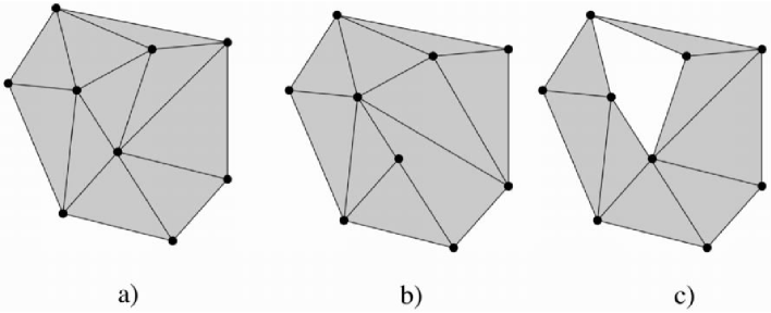
Figure 24: a) a valid triangulation, b) invalid since there are two triangles sharing only a part of a face, c) invalid because part of the domain is not covered by triangles

Voronoï diagram

A triangulation is not unique, as may be seen in figure 25.

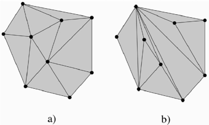
Figure 25: Two examples of valid triangulations for the same set of points. Intuitively, the a) case is “better” than the b) case

All triangulations are not equivalent for a given problem. There is a need to define a criterion of suitability. The most commonly used criterion is the Delaunay criterion which constraints the compactness of the triangles and will be explained later. It is linked to the so called Voronoï diagram. Given $\mathcal{S}$ a set of points $P_{i}$ in a $d$-dimensional space, the Voronoï diagram is the set of cells $\mathcal{V}_{i}$ associated with each point $P_{i}$ and defined as

$$\mathcal{V}_{i}=\{P\in\mathbb{R}^{n}\textrm{ such that }d(P,P_{i})\leq d(P,P_{j}),\forall j\neq i\}$$ (11)

Where $d$ is the euclidian distance between two points. In other words, $\mathcal{V}_{i}$ is the locus of points in $\mathbb{R}^{n}$ closer to $P_{i}$ than to any other point of $\mathcal{S}$. It has been shown [12] that the geometrical dual of the Voronoï diagram is a triangulation, the Delaunay triangulation (fig. 26).

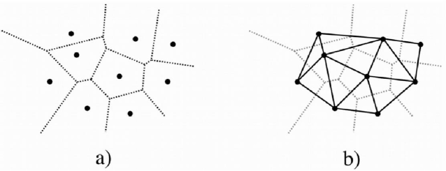
Figure 26: a) the Voronoï diagram of a set of points and b) the dual of the Voronoï diagram, the Delaunay triangulation

Delaunay triangulation

The Delaunay criterion states that the open circumdisk (in 2 dimensions, circumsphere in $n$ dimensions) of a triangle (simplex) contains no point from the set. The example in figure 27 shows a triangulation not satisfying the Delaunay criterion.

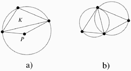
Figure 27: Example of a) a triangulation not satisfying the Delaunay criterion (the point $P$ is inside the circumdisk of $K$) b) satisfying it. A few circumcircles of triangles are shown

Among all possible triangulations, the Delaunay triangulation

• maximizes the minimum angle formed by the faces of the triangles

• minimizes the biggest diameter of the circumcircles associated with the triangles

Intuitively, this would mean that the Delaunay triangulation produces the more “compact” triangles.

A simple algorithm

Based on the previous definition of the Delaunay criterion, it is possible to devise a simple algorithm to compute a triangulation based on a set of points. It is called an incremental algorithm, or Bowyer-Watson algorithm [14][15].

The algorithm is incremental in the sense that the points of the set $S$ are added one by one, recomputing a triangulation at each step. The process starts by the generation of a supertriangle that encompasses all the points in $S$. At the end, all triangles that share one edge with the supertriangle are removed. The addition of one point is illustrated in figure 28

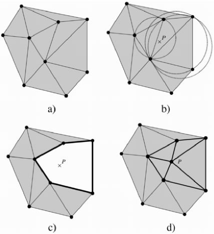
Figure 28: Incremental algorithm. a) add a point $P$ to an existing triangulation, b) remove all triangles whose circumcircle contains $P$, c) obtain a polygon enclosing P, d) triangulate only this polygon

To add one point $P$, all the triangles whose circumcircle contains $P$ are first removed. The resulting hole in the triangulation has a polygonal shape. New triangles are formed between $P$ and the outside edges of the polygon.

References

- [1] Search templates for gravitational waves from inspiraling binaries: Choice of template spacing, B.J.Owen, Physical Review D, 53(1996) 6749-6761
- [2] Virgo Coll., Final Design Report, 1997, see also http://www.virgo.infn.it/
- [3] See, e.g., N. Wiener,The Extrapolation, Interpolation and Smoothing of Stationary Time Series with Engineering Applications (Wiley, New York, 1949)
- [4] Filtering post-Newtonian gravitational waves from coalescing binaries, B.S. Sathyaprakash, Physical Review D, 50(1994) R7111-R7115
- [5] B.F. Schutz, in The Detection of Gravitational Radiation, Cambridge University Press, Cambridge, England, 1989
- [6] D.K. Churches,T. Cokelaer,B.S. Sathyaprakash Package Bank, Lal Software Documentation
- [7] Optimum Placement of Post-1PN GW Chirp Templates Made Simple at any Match Level via Tanaka-Tagoshi Coordinates, R.P. Croce, Th Demma, V. Pierro and I.M. Pinto, Physical Review D, 65(2002) 102003
- [8] Matched filtering of gravitational waves from inspiraling compact binaries: Computational cost and template placement, B.J.Owen and B.S. Sathyaprakash, Physical Review D, 60(1999) 022002
- [9] New contour reconstruction technique in template parameter space and associated placement, F. Beauville et al., Class. Quantum Grav., 20(2003) S789-S801
- [10] J. O’Rourke,Computational geometry in C (Cambridge University Press, Cambridge, 1998)
- [11] P.L. George, H. Borouchaki Triangulation de Delaunay et maillage (Hermes, Paris, 1997)
- [12] B. Delaunay (1934), Sur la sphère vide, Bul. Acad. Sci. URSS, Class. Sci. Nat., 793-800
- [13] http://www.lsc-group.phys.uwm.edu/lal/
- [14] D.F. Watson,Computing the -dimensional Delaunay tessellation with applications to Voronoi polytopes, The Computer Journal, 24(2) (1981) 167-172.
- [15] A. Bowyer,Computing Dirichlet tessellations, The Computer Journal, 24(2) (1981) 162-166.
- [16] B.F. Schutz, in The Detection of Gravitational Waves, Edited by D.G. Blair, Cambridge University Press, Cambridge, England, 1991, p.406
- [17] A. Viceré, Computational costs for coalescing binaries detection in Virgo using matched filters, Virgo Note, VIR-NOT-PIS-1390-149 (2000).
- [18] A faster implementation of the hierarchical search algorithm for detection of gravitational waves from inspiraling compact binaries, A.S. Sengupta, S. Dhurandhar and A. Lazzarini, Physical Review D, 67(2003) 082004
- [19] Elliptical tiling method to generate a 2-dimensional set of templates for gravitational wave search, N. Arnaud et al., Physical Review D, 67(2003) 102003