A time-domain MCMC search and upper limit technique for gravitational waves of uncertain frequency from a targeted neutron star.

Abstract

It is computationally expensive to search the large parameter space associated with a gravitational wave signal of uncertain frequency, such as might be expected from the possible pulsar generated by SN1987A. To address this difficulty we have developed a Markov Chain Monte Carlo method that performs a time-domain Bayesian search for a signal over a 4 Hz frequency band and a spindown of magnitude of up to $1\!\times\!10^{-9}$ Hz/s. We use Monte Carlo simulations to set upper limits on signal amplitude with this technique, which we intend to apply to a gravitational wave search.

1 Introduction

Recent targeted searches for gravitational waves from radio pulsars have needed to consider only four signal parameters: $h_{0}$, the signal amplitude, $\cos{\iota}$, the inclination angle of the pulsar toward the line of sight, $\psi$, the polarisation angle of the gravitational wave and $\phi_{0}$, the initial phase of the signal. In the absence of a detection, it is possible to set an upper limit on $h_{0}$, and therefore on the ellipticity of the pulsar in question. This is accomplished by defining a Bayesian posterior probability density function (PDF) of the four signal parameters and marginalising it numerically on a grid. In the time-domain, this search technique relies on precise heterodyning of data from the gravitational wave detector, which itself requires accurate information on the phase evolution of the signal. For known pulsars this is easily obtained by monitoring the timing of their radio wave pulses, which directly provides the frequency and frequency derivatives of the gravitational signal (emitted at twice the object’s rotation frequency) [1]. However, there are objects whose frequencies are not known accurately, such as the reported remnant of Supernova 1987A [3]. To perform a search over a range of frequencies would require a grid on frequency and frequency derivative with resolutions approximately $1/T_{\rm obs}$ and $1/T_{\rm obs}^{2}$ respectively, which makes the number of search templates very large ($\sim 4.5\!\times\!10^{11}$ for LIGO S3 data). We present an adaptation of this search based on a Markov Chain Monte Carlo (MCMC) method which does not require an exhaustive examination of the parameter space and therefore is able to search a range of frequencies in a reasonable time.

2 MCMC parameter estimation

After heterodyning at close to the expected signal frequency, the gravitational wave signal from a rotating triaxial neutron star has the form

$$y(t_{k};{\bf a})=\Big{(}\frac{1}{4}F_{+}(t_{k};\psi)(1+\cos^{2}\iota)-\frac{i}{2}F_{\times}(t_{k};\psi)\cos{\iota}\Big{)}h_{0}e^{i\Phi(t_{k})}$$ (1)

where $F_{+}$ and $F_{\times}$ are the beam patterns for the $+$ and $\times$ polarisations, and $\Phi(t)$ is the phase of the signal given to the first two Taylor expansion terms by

$$\Phi(t)=\phi_{0}+2\pi[\delta{}f(T-T_{0})+\frac{1}{2}\delta{}\dot{f}(T-T_{0})^{2}].$$ (2)

Here, $\delta{}f$ is the deviation of the signal frequency from the heterodyne frequency, and $\delta\dot{f}$ is the deviation from first derivative of the heterodyne frequency [7]. By including these two parameters we can search around the heterodyne frequency for a signal. The heterodyned data is reduced to one complex sample per minute, $B_{k}$, with variance $\sigma_{k}$, allowing a frequency range of $[-1/120,1/120]$ Hz around the heterodyne frequency to be searched. The search in $\delta\dot{f}$ is limited to $[-1\!\times\!10^{-9},1\!\times\!10^{-9}]$ Hz/s which is likely to include any possible pulsar spindown rates. The search proceeds by heterodyning 480 separate frequency bands at intervals of $1/120$ Hz, and running parallel searches on each band. In this way we complete a search over a 4 Hz range – suitable for the putative SN1987A pulsar.

The probability of a particular combination of the six parameters ${\bf a}$ representing a signal in the data $\{B_{k}\}$ is

$$p({\bf a}|\{B_{k}\})\propto p({\bf a})\exp{}\left[-\sum_{k}\frac{|B_{k}-y(t_{k};{\bf a})|^{2}}{2\sigma_{k}^{2}}\right],$$ (3)

which is the prior probability of ${\bf a}$ multiplied by its likelihood. This proportional definition is adequate for our application, as we will only be evaluating ratios of probabilities.

We now have a joint posterior probability distribution over the six parameters in vector ${\bf a}$, but in the presence of a signal the probability will be strongly concentrated around the signal parameters. The Markov Chain Monte Carlo method takes advantage of this fact by preferentially sampling the areas of greatest probability density, in proportion to that probability [4, 2]. In this way we can approximate the posterior distribution $p({\bf a}|\{B_{k}\})$ by allowing the Markov Chain to accumulate many samples, where the density of samples in an area is then proportional to the probability density in that area. In order to accomplish this, a Markov Chain in state ${\bf a}$ chooses a candidate sample ${\bf a^{\prime}}$ from proposal distribution $q_{1}({\bf a^{\prime}}|{\bf a})$, and then accepts the candidate as the next state of the chain with probability

$$\alpha_{1}({\bf a^{\prime}}|{\bf a})={\rm min}\left[1,\frac{p({\bf a^{\prime}})p(\{B_{k}\}|{\bf a^{\prime}})q_{1}({\bf a}|{\bf a^{\prime}})}{p({\bf a})p(\{B_{k}\}|{\bf a})q_{1}({\bf a^{\prime}}|{\bf a})}\right].$$ (4)

If the proposal is not accepted, the current state ${\bf a}$ is recorded as a sample again and the process repeats. The proposal distribution $q_{1}({\bf a^{\prime}}|{\bf a})$ is a multivariate normal distribution, with covariances determined by the correlation between parameters in trial runs. In practice, the highly correlated parameters $h_{0}$ and $\cos\iota$ are replaced with a re-parameterisation, such that $a_{1}=\frac{1}{4}h_{0}(1+\cos^{2}\iota)$ and $a_{2}=\frac{1}{2}h_{0}\cos\iota$. The frequency parameters are also changed to $f_{\rm start}=\delta{}f+\frac{1}{2}\delta\dot{f}\times{}t_{\rm start}$ and $f_{\rm end}=\delta{}f+\frac{1}{2}\delta\dot{f}\times{}t_{\rm end}$, being the signal frequency at the start and end times of the data.

It is important that the chain explore the parameter space adequately, in order to find the area of high probability. To this end, we have included a delayed rejection stage of the algorithm, so that if a proposal ${\bf a^{\prime}}$ is rejected, a new candidate is generated from distribution $q_{2}({\bf a^{\prime\prime}}|{\bf a^{\prime}},{\bf a})$, which has a narrower width and makes more conservative steps. These are accepted with probability

$$\alpha_{2}({\bf a^{\prime\prime}}|{\bf a})={\rm min}\left[1,\frac{p({\bf a^{\prime\prime}})p(\{B_{k}\}|{\bf a^{\prime\prime}})q_{1}({\bf a^{\prime}}|{\bf a^{\prime\prime}})q_{2}({\bf a}|{\bf a^{\prime}},{\bf a^{\prime\prime}})(1-\alpha_{1}({\bf a^{\prime}}|{\bf a^{\prime\prime}}))}{p({\bf a})p(\{B_{k}\}|{\bf a})q_{1}({\bf a^{\prime}}|{\bf a})q_{2}({\bf a^{\prime\prime}}|{\bf a},{\bf a^{\prime}})(1-\alpha_{1}({\bf a^{\prime}}|{\bf a}))}\right],$$ (5)

where the proposal distributions are included to satisfy the principle of detailed balance. This allows the chain to make small steps where a large step would be rejected.

In addition to these measures, there is also a burn-in period at the start of each MCMC run where the exponent in Eqn. 3 is multiplied by an inverse temperature factor $\beta$ in the proposed step. Initially $\beta=0.01$, and gradually increases during the burn-in period to $\beta=1$, where Eqn. 3 is restored. This decreases the likelihood of the chain getting stuck in a local maximum of probability without exploring the space adequately. No samples from the burn-in period are used in calculating the final PDF, as they do not represent the target distribution $p({\bf a}|\{B_{k}\})$. In our implementation the burn-in lasts for $1\!\times\!10^{6}$ iterations, followed by 100 000 iterations with every 50th used as a sample, so as to reduce correlation between samples. The program is implemented in C, using the LIGO Algorithm Library to calculate the beam patterns and time delays necessary for analysing a real signal [5].

3 Setting upper limits

In the standard time-domain search, if a signal is not detected it is useful to set an upper limit on gravitational radiation emitted by the source under examination. This translates as an upper limit on the ellipticity of the pulsar which can be used to constrain physical models of a neutron star. This is achieved by marginalising the posterior PDF over $\cos\iota$, $\psi$ and $\phi_{0}$, leaving a distribution on $h_{0}$ which can then be integrated upward from $h_{0}=0$ until 95% of the probability is included in the interval. The upper limit of the interval is then the 95% upper limit on $h_{0}$ for the target.

In the MCMC routine however, if the signal is below a certain threshold then the chain may not converge on the correct mode of the signal in the PDF [6]. This is partly due to the narrowness of the mode in $\delta{}f$ and $\delta\dot{f}$, where the bulk of the probability lies within a single frequency bin of width $1/T_{\rm obs}$ with a very small attraction area.

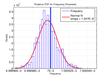
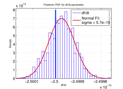
Figure 1: The posterior PDFs (bars) for a 2000 sample chain which has converged on the injected values of $\delta{}f=7\!\times\!10^{-3}$ Hz and $\delta\dot{f}=-2.5\!\times\!10^{-10}$ Hz/s (vertical lines), and the best normal fits, having standard deviations $1.047\!\times\!10^{-8}$ Hz and $5.7031\!\times\!10^{-15}$ Hz/s respectively.

A weak signal will raise probability only slightly in this bin, so that even if the chain were to find the mode, it has a probability of jumping out and not returning. These factors therefore preclude the evaluation of an upper limit simply by marginalising the posterior PDF when there is no detection. Instead, we performed a Monte Carlo simulation by injecting signals of known parameters into noise, and running the MCMC code to try and recover them. Signals are injected with known parameters by calculating the value of the signal at each timestamp $t_{k}$ using LAL and adding it to each sample $B_{k}$ in the input data file. Real data would have to be heterodyned prior to this step, but the artificial noise is generated at $1/60$ Hz so heterodyning is unnecessary in the simulations. It can be shown that the probability of detecting a signal using our method depends strongly on the injected values of $h_{0}$ and $\cos\iota$, and much more weakly on the value of $\psi$. To determine our upper limit for a particular set of data, we inject signals of varying $h_{0}$ and $\cos\iota$ into the noise $\sigma_{k}$, then analyse the results of the MCMC routine to determine if it has detected the signal. This is accomplished by observing the output PDFs in $\delta{}f$ and $\delta\dot{f}$, and determining if the chain has converged or not. If the injected value lies within three standard deviations of the mean, and the standard deviations themselves are less than one frequency bin in size, the chain is judged to have converged. If the chain has not converged, the samples are distributed widely over the entire $\delta{}f$ range, and the standard deviation is typically five orders of magnitude higher. Fig. 1 shows the posterior PDFs in the $\delta{}f$ and $\delta\dot{f}$ parameters for a chain converged on a signal with injected parameters $h_{0}=1.3$, $\cos\iota=0$, $\psi=0.281$, $\phi_{0}=4.234$, $\delta{}f=7\!\times\!10^{-3}$ Hz and $\delta\dot{f}=-2.5\!\times\!10^{-10}$  Hz/s, where the noise level was $\sigma=1.0$. Fig. 2 shows the same type of plot for a signal with $h_{0}=0.7$ and otherwise identical parameters; this chain failed to converge, so there is no concentrated mode in the PDF. The attempted fit to a normal distribution to test convergence is therefore very wide, and poorly fitted.

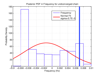
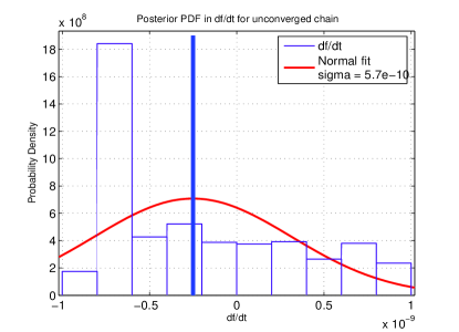
Figure 2: The $\delta{}f$ and $\delta\dot{f}$ posterior PDFs (bars) for a 2 000 sample chain which failed to converge on the injected parameters (vertical lines). This distribution is clearly distinguishable from the converged case using the criteria defined above.

The injections are repeated, using a different starting point in parameter space for the MCMC chain each time, and an empirical probability of signal recovery $P(\rm detection|h_{0},\cos\iota,\sigma_{k})$ for each point on the ($h_{0}$, $\cos\iota$) plane is obtained from the set of results. Fig. 3 shows the result on the ($h_{0}$, $\cos\iota$) plane of performing this procedure on 64 000 samples of white noise with a variance of $\sigma=1.0$. The dark region shows where no signal is detectable, above which is a small transition zone where there is a finite probability of detection. With increasing iterations of the chain, the width of this zone reduces - we are using a chain of 1 100 000 iterations, of which the first 1 000 000 are burn-in time and the last 100 000 used for sampling the PDF. The white area above this transition zone represents signals that are detected with very high probability. These are strong enough to cause the chain to converge on them in every instance of the Monte Carlo simulation. It is clear from the figure that this is strongly dependent on $\cos\iota$, as this acts a weighting factor between the power in the real and imaginary parts of the heterodyned signal. The distribution is symmetric about $\cos\iota=0$, so only the positive half was calculated.

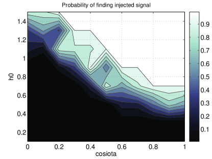
Figure 3: Results of Monte Carlo evaluation of probability of detection of a signal injected with varying values of $h_{0}$ and $\cos\iota$. This shows the strong dependence on both these parameters. The transition from detectable to undetectable occurs over a narrow region for a particular value of $\cos\iota$, but decreases in $h_{0}$ as $\cos\iota$ tends to 1.

This result can then be marginalised by summing over $\cos\iota$ and normalising to give a distribution on $h_{0}$, as required for an upper limit. The probability of there being an undetected gravitational wave is then $1-P(\rm detection|h_{0},\sigma_{k})$, and the upper limit $h_{95\%}$ satisfies $1-P(\rm detection|h_{95\%},\sigma_{k})=0.95$. Note that $P(\cdot|\cdot)$ is a probability rather than a probability density. The upper limit determined from this stage is applicable to each of the 480 bands in the 4 Hz frequency interval because the values of $\sigma_{k}$ are determined by estimating the noise over the entire 4 Hz band at the heterodyne stage. The heterodyne then performs filtering of this band to calculate the signal $B_{k}$ in each $1/60$ Hz interval, from which the 480 bands are derived.

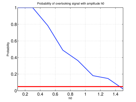
Figure 4: The marginalisation of Fig. 3 onto the $h_{0}$ axis. This shows that the 95% confidence (represented by the horizontal line) may be drawn at $h_{95\%}=1.44$.

Fig. 4 shows this final distribution on $h_{0}$, where the horizontal line represents 95% confidence in detection, required for a 95% upper limit, which is achieved at $h_{0}=1.44$. It is useful to express this in terms of noise power spectral density, $S_{h}$, yielding the relation

$$h_{95\%}=515.2\sqrt{\frac{S_{h}}{T_{\rm obs}}}{Hz}^{-\frac{1}{2}}.$$ (6)

where the 512.2 is an indicator of the sensitivity of the search, empirically derived from the simulation.

For a realistic example, consider a noise power spectral density of $S(f)=6.6\!\times\!10^{-44}\,{\rm Hz}^{-1}$, or $h(f)=2.57\!\times\!10^{-22}$, and a data run of 44 days, the upper limit would then be approximately

$$h_{95\%}=515.2\sqrt{\frac{6.6\!\times\!10^{-44}}{3801600}}=6.8\!\times\!10^{-23}{Hz}^{-\frac{1}{2}}.$$ (7)

4 Summary

This MCMC search method is capable of reliably detecting a signal above a certain threshold and estimating its parameters including frequency and spindown. The computing time it takes to perform the search is dependent only on the amount of data and the number of MCMC iterations desired, which provides significant improvement over the previous time-domain targeted search[8]. With the current version of the pipeline, to analyse the entire 4 Hz window would take about 17 000 CPU hours on a 1.8 GHz Athlon processor, which is approximately two days on the 366-CPU Merlin cluster at AEI Golm. In the absence of a signal an upper limit can be set using Monte Carlo injections, which require a similar amount of processing on top of the search itself. Additional work is under way to tune the algorithm further, which may lead to improvements in sensitivity and speed of execution.

We hope that this technique could be applied to a search for gravitational radiation from possible pulsar in the remnant of SN1987A at $935\pm 2$ Hz, and in the absence of detection place upper limits on the gravitational radiation emitted by this object if it were triaxial. The method could also be easily applied to other similar objects.

References

References

- [1] Abbot B et al(The LIGO Scientific Collaboration) 2004 Phys. Rev. D 69 082004
- [2] Richard Umstätter, Renate Meyer, Réjean J Dupuis, John Veitch, Graham Woan and Nelson Christensen 2004 Class. Quantum Grav. 21 No 20 S1655-S1665
- [3] J. Middleditch, J. A. Kristian, W. E. Kunkel et al. Rapid photometry of supernova 1987A: a 2.14 ms pulsar? New Astronomy 5:243-283, August 2000
- [4] D. Gamerman. Markov Chain Monte Carlo: Stochastic Simulation for Bayesian Inference. Chapman & Hall, 1997
- [5] http://www.lsc-group.phys.uwm.edu/lal/
- [6] W.R. Gilks and S. Richardson and D.J. Spiegelhalter, Markov Chain Monte Carlo in Practice (Chapman and Hall, London, 1996).
- [7] Jaranowski P, Królak A and Schutz B 1998 Phys. Rev. D 58 063001
- [8] Abbott B et al(The LIGO Scientific Collaboration), Kramer M and Lyne A, accepted by Phys. Rev. Lett. Preprint gr-qc/0410007.