Wave and Particle Scattering Properties of High Speed Black Holes

Abstract

The light–like limit of the Kerr gravitational field relative to a distant observer moving rectilinearly in an arbitrary direction is an impulsive plane gravitational wave with a singular point on its wave front. By colliding particles with this wave we show that they have the same focussing properties as high speed particles scattered by the original black hole. By colliding photons with the gravitational wave we show that there is a circular disk, centered on the singular point on the wave front, having the property that photons colliding with the wave within this disk are reflected back and travel with the wave. This result is approximate in the sense that there are observers who can see a dim (as opposed to opaque) circular disk on their sky. By colliding plane electromagnetic waves with the gravitational wave we show that the reflected electromagnetic waves are the high frequency waves.

1 Introduction

When the Kerr black hole, located at the spatial origin of coordinates $\{\bar{x},\bar{y},\bar{z},\bar{t}\}$, has its axis pointing in an arbitrary direction relative to this asymptotically rectangular Cartesian coordinate system the metric tensor is given in Kerr–Schild form by

$$\bar{g}_{\mu\nu}=\bar{\eta}_{\mu\nu}+2\,H\,\bar{k}_{\mu}\,\bar{k}_{\nu}\ ,$$ (1.1)

with $\bar{\eta}_{\mu\nu}={\rm diag}(1,1,1,-1)$,

$$H=\frac{m\,\bar{r}^{3}}{\bar{r}^{4}+({\bf a}\cdot\bar{\bf x})^{2}}\ ,$$ (1.2)

and

$$\bar{k}_{\mu}\,d\bar{x}^{\mu}=\frac{({\bf a}\cdot\bar{\bf x})\,({\bf a}\cdot d\bar{\bf x})}{\bar{r}\,(\bar{r}^{2}+|{\bf a}|^{2})}+\frac{\bar{r}\,(\bar{\bf x}\cdot\bar{\bf dx})}{\bar{r}^{2}+|{\bf a}|^{2}}-\frac{{\bf a}\cdot({\bf\bar{x}}\times d{\bf\bar{x}})}{(\bar{r}^{2}+|{\bf a}|^{2})}-d\bar{t}\ .$$ (1.3)

Here ${\bf a}=(c,b,a)$, with $|{\bf a}|^{2}=a^{2}+b^{2}+c^{2}$ and $\bar{\bf x}=(\bar{x},\bar{y},\bar{z})$ with $\bar{r}$ given in terms of $\bar{x},\bar{y},\bar{z}$ by

$$\bar{x}^{2}+\bar{y}^{2}+\bar{z}^{2}+\frac{(c\bar{x}+b\bar{y}+a\bar{z})^{2}}{\bar{r}^{2}}=\bar{r}^{2}+a^{2}+b^{2}+c^{2}\ .$$ (1.4)

The dot and cross above signify the usual scalar and vector product in three–dimensional Euclidean space. This form of the Kerr metric has been given by Weinberg [1] and a derivation is given in [2]. When we consider the deflection of a highly relativistic particle in the Kerr gravitational field [2] we proceed as follows: The direction of the incoming particle is parallel to the positive $\bar{x}$–axis. The particle is projected with 3–velocity $v$ at a large distance from the black hole and with a non–zero (large) impact parameter. Since the black hole axis points in an arbitrary direction, projecting a particle in the $\bar{x}$–direction is equivalent to projecting in an arbitrary direction. We call $\bar{S}$, with coordinates $\{\bar{x},\bar{y},\bar{z},\bar{t}\}$, the rest frame of the Kerr source and $S$, with coordinates $\{x,y,z,t\}$, the rest–frame of the high speed particle. These frames are related by the Lorentz boost in the $\bar{x}$–direction

$$\bar{x}=\gamma\,(x+v\,t)\ ,\qquad\bar{y}=y\ ,\qquad\bar{z}=z,\qquad\bar{t}=\gamma\,(t+v\,x)\ ,$$ (1.5)

with $\gamma=(1-v^{2})^{-1/2}$. In $S$ the particle sees the Kerr source moving towards it with a speed close to the speed of light (unity in our units). In the ultrarelativistic limit the Kerr gravitational field looks to the particle as the gravitational field of a plane–fronted impulsive gravitational wave. The line–element of the space–time model of this field is derived in [2] and can be written in the form

$$ds^{2}=dx^{2}+dy^{2}+dz^{2}-dt^{2}-2\,H\,(dx+dt)^{2}\ ,$$ (1.6)

with

$$H=h(y,z)\,\delta(x+t)\ ,\qquad h(y,z)=2p\,\log\{(y-a)^{2}+(z+b)^{2}\}\ ,$$ (1.7)

with $p,a,b$ constants. The gravitational field described by (1.6) and (1.7) results in the limit $v\mapsto 1$ with the mass $m$ of the black hole tending to zero in this limit in such a way that $m\,(1-v^{2})^{-1/2}\mapsto p$. Here $b,a$ are respectively the components of the angular momentum per unit mass of the black hole in the $y$ and $z$ directions. The component of the angular momentum per unit mass in the $x$ direction drops out in the light–like limit on account of the way in which it must scale in terms of $v$ due to Lorentz contraction (this is explained in terms of the behavior of the multipole moments of the isolated source in [3], [4]). The hyperplane $x+t=0$ is null and the Riemann tensor of the space–time has components which are multiples of the Dirac delta function $\delta(x+t)$. This tensor is Type N in the Petrov classification and $x+t=0$ is the history of a plane impulsive gravitational wave. As well as being singular on the null hyperplane $x+t=0$ the Riemann tensor is also singular at $y=a,\ z=-b$ which is the singularity of the logarithm in (1.2). This is a null geodesic generator of the hyperplane $x+t=0$ and is a singular point on the plane wave front. When $a=b=0$ (1.6), (1.7) reduces to the gravitational field of the Schwarzschild source boosted to the speed of light originally calculated by Aichelburg and Sexl [5].

In this paper we demonstrate in section 2 that the focussing behavior of a time–like congruence in the space–time with line–element (1.6) is exactly what one would expect in the field of a rotating source. The focussing of geodesics in the space–time of general plane gravitational waves has been discussed in [6]. In section 3 we calculate the behavior of photons (a null geodesic congruence) which experience a head–on collision with the impulsive gravitational wave described by (1.6) and (1.7) as a prelude to the study of the collision of plane electromagnetic waves with the gravitational wave. This enables us to demonstrate in section 4 the dimming of the light signal by the gravitational wave and to indicate that it is the high electromagnetic wave frequencies being reflected by the gravitational wave that is responsible for the dimming. When studying photons and electromagnetic waves in the present paper we solve the null geodesic equations and Maxwell’s equations in the space–time given by (1.6) and (1.7). This is required in order to describe the new signal dimming phenomenon which applies to a non–rotating as well as to a rotating black hole.

2 Scattering of Particles:Time-Like Geodesics

The time–like geodesic equations in the space–time with line–element (1.6) with (1.7) can be used to calculate the angles of deflection of a high speed particle projected in any direction into the field of the black hole [2] [7]. This involves two approximations: in the rest frame of the incoming particle the Kerr field is taken to be given approximately by (1.6) with (1.7) and the impact parameter must be large. The leading terms in the calculated deflection angles are found to coincide with the angles of deflection of photons projected into the Kerr field [2].

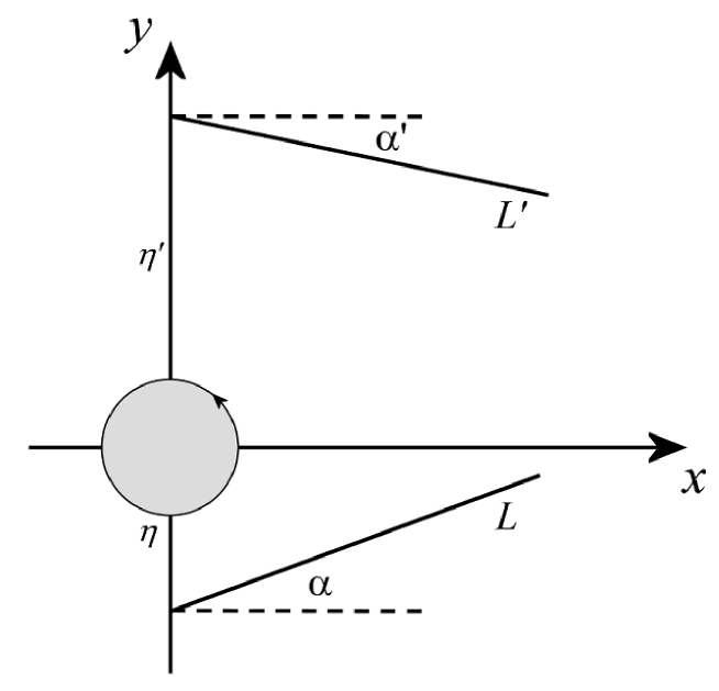
Figure 1: The equatorial plane $z=0$ with $a>0$ and thus the angular momentum points in the positive $z$-direction

The calculations are simplest when the particle is projected into the equatorial plane of the hole. For a Kerr black hole of mass $m$ and angular momentum ${\rm J}=(0,0,m\,a)$, with respect to asymptotically Cartesian spatial coordinates, Figure 1 shows the asymptotes $L$ and $L^{\prime}$ of two scattered photon paths in the equatorial plane, one co-rotating with the hole $(L)$ and one counter-rotating with the hole $(L^{\prime})$. The small angles of scattering $\alpha$ and $\alpha^{\prime}$ indicated in the figure have been calculated by Boyer and Lindquist [8] and are found to be

$$\alpha=\frac{4\,m}{\eta}-\frac{4\,m\,a}{\eta^{2}}>0\ ,$$ (2.1)

and

$$\alpha^{\prime}=-\frac{4\,m}{\eta^{\prime}}-\frac{4\,m\,a}{\eta^{\prime 2}}<0\ ,$$ (2.2)

respectively, where $\eta>0$ and $\eta^{\prime}>0$ are large impact parameters. To have $\alpha^{\prime}=-\alpha$ we see that we must have $\eta^{\prime}=\eta+2\,a$. In this case for $x\geq 0$ the straight lines $L$ and $L^{\prime}$ intersect on the straight line

$$y=a,\qquad z=0\ .$$ (2.3)

This asymmetrical behavior is entirely due to the rotation of the black hole. If $a=0$ then $\eta^{\prime}=\eta$ and $L$ and $L^{\prime}$ will intersect on the straight line $y=0$. The corresponding angles of deflection of high speed particles, calculated using the time–like geodesics of (1.6) with (1.7) are given exactly by [7]

$$\tan\alpha=\frac{4\,m\,(\eta+a)}{(\eta+a)^{2}-4\,m^{2}}\ ,$$ (2.4)

and

$$\tan\alpha^{\prime}=-\frac{4\,m\,(\eta^{\prime}-a)}{(\eta^{\prime}-a)^{2}-4\,m^{2}}\ ,$$ (2.5)

respectively. Putting $\alpha^{\prime}=-\alpha$ we deduce from these equations that

$$\eta^{\prime}=\eta+2\,a\ ,$$ (2.6)

without the assumption that $\eta,\ \eta^{\prime}$ are large and so $L$ and $L^{\prime}$ intersect on the straight line $y=a,\ z=0$ in this case also. We note that (2.4) and (2.5) agree with (2.1) and (2.2) if the impact parameters are large. This asymmetrical intersection behavior can be seen in greater generality by studying the deflection of a family of high speed particles projected into the field of the Kerr black hole. This involves the study of time–like geodesics of the space–time with line–element given by (1.6) and (1.7).

The time–like geodesic equations for the space–time described by (1.6) and (1.7) have been solved in [7]. If $\tau$ is proper time along them then we shall take $\tau<0$ on a geodesic before it intersects the null hyperplane $x+t=0$, $\tau=0$ at the point of intersection with $x+t=0$ and $\tau>0$ to the future of $x+t=0$. For the simplest initial conditions we find that a time–like geodesic is given for $\tau<0$ by

$$x = x_{0}+x_{1}\tau\ ,$$ (2.7)

$$y = y_{0}\ ,$$ (2.8)

$$z = z_{0}\ ,$$ (2.9)

$$t = -x_{0}+t_{1}\tau\ ,$$ (2.10)

and for $\tau>0$ by

$$x = x_{0}+x_{1}\tau+X_{1}\tau+\hat{X}_{1}\ ,$$ (2.11)

$$y = y_{0}+Y_{1}\tau\ ,$$ (2.12)

$$z = z_{0}+Z_{1}\tau\ ,$$ (2.13)

$$t = -x_{0}+t_{1}\tau-X_{1}\tau-\hat{X}_{1}\ ,$$ (2.14)

with

$$\hat{X}_{1} = (h)_{0}\ ,$$ (2.15)

$$X_{1} = -\frac{C_{0}}{2}\,\{(h_{y})_{0}^{2}+(h_{z})_{0}^{2}\}\ ,$$ (2.16)

$$Y_{1} = -C_{0}\,(h_{y})_{0}\ ,$$ (2.17)

$$Z_{1} = -C_{0}\,(h_{z})_{0}\ ,$$ (2.18)

and

$$x_{1}+t_{1}=C_{0}\ ,\qquad x_{1}-t_{1}=-C_{0}^{-1}\ ,$$ (2.19)

where $C_{0}$ is a constant. Here $h(y,z)$ is given by (1.7), subscripts $y$ and $z$ on $h$ indicate partial derivatives and round brackets followed by a subscript zero indicate that $h$ and its partial derivatives are to be evaluated at $y=y_{0},\ z=z_{0}$. By varying $x_{0},y_{0},z_{0}$ we have here two time–like congruences, one for $\tau<0$ and another for $\tau>0$. The interesting one corresponds to $\tau>0$ and the unit time–like tangent to the congruence on $\tau=0$ has components (in rectangular Cartesian coordinates and time; here and throughout Greek indices take values 1, 2, 3, 4)

$$v^{\mu}=(x_{1}+X_{1}\ ,\ Y_{1}\ ,Z_{1}\ ,\ t_{1}-X_{1})\ .$$ (2.20)

We can consider (2.11)–(2.14) defining $x_{0},\ y_{0},\ z_{0},\ \tau$ as scalar fields on the region of Minkowskian space–time $\tau\geq 0$. Thus $v^{\mu}$ becomes a vector field on $\tau\geq 0$ whose integral curves constitute the congruence of interest. In addition we can use $x_{0},\ y_{0},\ z_{0},\ \tau$ as coordinates on this region of space–time, which we label by $X^{\mu}=(\zeta\ ,\bar{\zeta}\ ,x_{0}\ ,\tau)$ with $\zeta=y_{0}+iz_{0}$. In these coordinates (2.20) is given via the 1–form

$$v_{\mu}\,dX^{\mu}=C_{0}\,dx_{0}-d\tau\ ,$$ (2.21)

or alternatively as the covariant vector field

$$v^{\mu}\,\frac{\partial}{\partial X^{\mu}}=\frac{\partial}{\partial\tau}\ .$$ (2.22)

The line–element in the region $\tau\geq 0$ of Minkowskian space–time is given by

$$ds^{2} = dx^{2}+dy^{2}+dz^{2}-dt^{2}\ ,$$ (2.23)

$$= \left|d\zeta-2\,C_{0}\,\tau\,\frac{\partial^{2}(h)_{0}}{\partial\bar{\zeta}^{2}}\,d\bar{\zeta}\right|^{2}+2\,C_{0}\,d\tau\,dx_{0}-d\tau^{2}\ .$$

Before the time–like congruence encounters the null hyperplane history of the impulsive gravitational wave (for $\tau<0$) it is given parametrically by (2.7)–(2.10). Again using $x_{0},y_{0},z_{0},\tau$ as cordinates the line–element of Minkowskian space–time for $\tau<0$ is given by

$$ds^{2}=|d\zeta|^{2}+2\,C_{0}\,d\tau\,dx_{0}-d\tau^{2},$$ (2.24)

where as before $\zeta=y_{0}+iz_{0}$. The two line–elements (2.23) and (2.24) can be combined to read

$$ds^{2}=\left|d\zeta-2\,C_{0}\,\tau\,\vartheta(\tau)\,\frac{\partial^{2}(h)_{0}}{\partial\bar{\zeta}^{2}}\,d\bar{\zeta}\right|^{2}+2\,C_{0}\,d\tau\,dx_{0}-d\tau^{2}\ .$$ (2.25)

Here $\vartheta(\tau)$ is the Heaviside step function (equal to unity if $\tau>0$ and equal to zero if $\tau<0$) and now this line–element incorporates the impulsive gravitational wave with history $\tau=0$. The metric tensor in these coordinates is clearly continuous across $\tau=0$ but has a jump in its first derivative across $\tau=0$ and the Riemann curvature tensor will have a delta function singular on $\tau=0$. This can easily be checked by direct calculation starting with the line–element (2.25).

To work out the properties of the time–like congruence (contraction, twist and shear) for $\tau>0$, having as tangent the covariant vector field (2.21), we need the covariant derivative of the tangent with respect to the Riemannian connection calculated with the metric tensor given via the line–element (2.25) with $\tau>0$. With this derivative indicated by a stroke, we find that it takes the neat form

$$v_{\mu|\nu}=\hat{\mu}_{1}\,n_{(1)\mu}\,n_{(1)\nu}+\hat{\mu}_{2}\,n_{(2)\mu}\,n_{(2)\nu}=v_{\nu|\mu}\ .$$ (2.26)

Here $n_{(1)\mu}\ ,n_{(2)\mu}$ are given via the 1–forms

$$n_{(1)\mu}\,dX^{\mu} = \frac{i}{2}(1+2\,C_{0}\,\tau\,|h_{\zeta\zeta}|)\,\left\{\left(\frac{h_{\zeta\zeta}}{|h_{\zeta\zeta}|}\right)^{\frac{1}{2}}d\zeta-\left(\frac{|h_{\zeta\zeta}|}{h_{\zeta\zeta}}\right)^{\frac{1}{2}}d\bar{\zeta}\right\}\ ,$$ (2.27)

$$n_{(2)\mu}\,dX^{\mu} = \frac{1}{2}(1-2\,C_{0}\,\tau\,|h_{\zeta\zeta}|)\,\left\{\left(\frac{h_{\zeta\zeta}}{|h_{\zeta\zeta}|}\right)^{\frac{1}{2}}d\zeta+\left(\frac{|h_{\zeta\zeta}|}{h_{\zeta\zeta}}\right)^{\frac{1}{2}}d\bar{\zeta}\right\}\ ,$$ (2.28)

where here and henceforth we use the shorthand

$$h_{\zeta\zeta}=\frac{\partial^{2}(h)_{0}}{\partial\zeta^{2}}\ .$$ (2.29)

The vectors $n^{\mu}_{(1)}\ ,\ n^{\mu}_{(2)}$ are unit space–like vectors, orthogonal to each other and each orthogonal to $v^{\mu}$. They are both parallel transported along the congruence tangent to $v^{\mu}$. We thus confirm from (2.26) that the congruence is geodesic and twist–free. The scalars $\hat{\mu}_{1},\ \hat{\mu}_{2}$ in (2.26) are given by

$$\hat{\mu}_{1} = \frac{2\,C_{0}\,|h_{\zeta\zeta}|}{1+2\,C_{0}\,\tau\,|h_{\zeta\zeta}|}\ ,$$ (2.30)

$$\hat{\mu}_{2} = \frac{-2\,C_{0}\,|h_{\zeta\zeta}|}{1-2\,C_{0}\,\tau\,|h_{\zeta\zeta}|}\ .$$ (2.31)

Hence the contraction of the congruence is given by

$$\vartheta=v^{\mu}{}_{|\mu}=\hat{\mu}_{1}+\hat{\mu}_{2}=-\frac{8\,C_{0}^{2}\tau\,|h_{\zeta\zeta}|^{2}}{1-4C_{0}^{2}\tau^{2}|h_{\zeta\zeta}|^{2}}\ .$$ (2.32)

The shear tensor $\sigma_{\mu\nu}$ associated with the congruence reads now

$$\sigma_{\mu\nu}=v_{\mu|\nu}-\frac{1}{3}\vartheta\,(g_{\mu\nu}+v_{\mu}\,v_{\nu})\ .$$ (2.33)

An orthonormal tetrad which is parallel propagated along the congruence is given by $\{n_{(1)}^{\mu},n_{(2)}^{\mu},n^{\mu},v^{\mu}\}$ with the unit space–like vector field $n^{\mu}$ given by

$$n^{\mu}\,\frac{\partial}{\partial X^{\mu}}=C_{0}^{-1}\frac{\partial}{\partial x_{0}}+\frac{\partial}{\partial\tau}\ .$$ (2.34)

Using (2.26) and (2.33) we can write the shear tensor in the form

$$\sigma_{\mu\nu}=\mu_{1}\,n_{(1)\mu}\,n_{(1)\nu}+\mu_{2}\,n_{(2)\mu}\,n_{(2)\nu}+\mu_{3}\,n_{\mu}\,n_{\nu}\ ,$$ (2.35)

with

$$\mu_{1}=\hat{\mu}_{1}-\frac{1}{3}\vartheta\ ,\mu_{2}=\hat{\mu}_{2}-\frac{1}{3}\vartheta\ ,\mu_{3}=-\frac{1}{3}\vartheta\ .$$ (2.36)

We note that $\{n_{(1)}^{\mu},n_{(2)}^{\mu},n^{\mu},v^{\mu}\}$ are the unit eigenvectors of the shear tensor with $\{\mu_{1},\mu_{2},\mu_{3},0\}$ the corresponding eigenvalues. The shear tensor is trace free in the sense that $g^{\mu\nu}\,\sigma_{\mu\nu}=0$ and thus $\mu_{1}+\mu_{2}+\mu_{3}=0$ and this follows from (2.32). This time–like congruence is an approximation to the world lines of high speed particles after they have been deflected by the rotating black hole. That it exhibits the intersection behavior described at the beginning of this section (actually a generalization of this behavior because the congruence above has resulted from the scattering of high speed particles projected at any angle into the field of the black hole) can be seen easily by first noting from (2.32) that the lines of the congruence converge when $\tau=\tau_{0}$ with $\tau_{0}$ given by

$$\tau_{0}=\frac{(y_{0}-a)^{2}+(z_{0}+b)^{2}}{4\,C_{0}\,p}\ .$$ (2.37)

However from (2.12) and (2.13) we have

$$y-a = (y_{0}-a)\,\left(1-\frac{\tau}{\tau_{0}}\right)\ ,$$ (2.38)

$$z+b = (z_{0}+b)\,\left(1-\frac{\tau}{\tau_{0}}\right)\ ,$$ (2.39)

and the right hand sides of these equations vanish when $\tau=\tau_{0}$ given by (2.37). Thus in this more general case the paths of the high speed particles converge on a straight line after being scattered by the black hole and this straight line is the intersection of the planes $y=a,\ z=-b$.

3 Scattering of Particles:Null Geodesics

We will consider in section 4 the collision of plane electromagnetic waves propagating in the positive $x$–direction with the impulsive gravitational wave (1.6) with (1.7) which is propagating in the negative $x$–direction. We will treat the electromagnetic field of the waves before and after collision as a test field on this space–time. We show in an appendix that it is always possible to find a frame of reference in which this collision is head–on. As a prelude to this we examine in this section the behavior of null geodesics in the space–time described by (1.6) and (1.7). The light–like propagation direction of the electromagnetic waves before encountering the impulsive gravitational wave is given (in rectangular Cartesian coordinates and time $x,y,z,t$) by

$${}^{(-)}l^{\mu}=(1,0,0,1)\ .$$ (3.1)

The superscript minus on $l$ denotes a quantity before collision with the gravitational wave. A useful null tetrad is given by $\{{}^{(-)}l^{\mu},{}^{(-)}n^{\mu},{}^{(-)}m^{\mu},{}^{(-)}\bar{m}^{\mu}\}$ with

$${}^{(-)}n^{\mu}=\left(\frac{1}{2},0,0,-\frac{1}{2}\right)\ ,\qquad{}^{(-)}m^{\mu}=\frac{1}{\sqrt{2}}(0,1,i,0)\ ,$$ (3.2)

and ${}^{(-)}\bar{m}^{\mu}$ the complex conjugate of ${}^{(-)}m^{\mu}$. All scalar products among $\{{}^{(-)}l^{\mu},{}^{(-)}n^{\mu},{}^{(-)}m^{\mu},{}^{(-)}\bar{m}^{\mu}\}$ vanish with the exception of ${}^{(-)}n^{\mu}\,{}^{(-)}l_{\mu}=1$ and ${}^{(-)}\bar{m}^{\mu}\,{}^{(-)}m_{\mu}=1$. As a preliminary we investigate what happens a null geodesic starting with tangent ${}^{(-)}l^{\mu}$ in the space–time with line–element (1.6). The differential equations of such a curve $x^{\mu}=x^{\mu}(\lambda)$, where $\lambda$ is an affine parameter, are

$$\ddot{x} = H_{x}\,(\dot{x}+\dot{t})^{2}+2\,(h_{y}\dot{y}+h_{z}\dot{z})\,(\dot{x}+\dot{t})\,\delta(x+t)\ ,$$ (3.3)

$$\ddot{y} = -h_{y}\,(\dot{x}+\dot{t})^{2}\delta(x+t)\ ,$$ (3.4)

$$\ddot{z} = -h_{z}\,(\dot{x}+\dot{t})^{2}\delta(x+t)\ ,$$ (3.5)

$$\ddot{t} = -H_{x}\,(\dot{x}+\dot{t})^{2}-2\,(h_{y}\dot{y}+h_{z}\dot{z})\,(\dot{x}+\dot{t})\,\delta(x+t)\ .$$ (3.6)

As always subscripts on $H$ and $h$ denote partial derivatives and, in particular, $H_{x}=h(y,z)\,\delta^{\prime}(x+t)$, with the prime on the delta function denoting the derivative with respect to the argument of the function. Differentiation with respect to $\lambda$ is indicated by a dot. The first integral of (3.3)–(3.6) is given by

$$(\dot{x}+\dot{t})\,\{\dot{x}-\dot{t}-2\,H\,(\dot{x}+\dot{t})\}+\dot{y}^{2}+\dot{z}^{2}=0\ .$$ (3.7)

These equations are identical in form to the time–like geodesic equations in this space–time considered in [7], with the exception of a zero appearing on the right hand side of (3.7) instead of minus one. They are solved in exactly the same way. If $\lambda<0$ on the null geodesic before encountering the null hyperplane $x+t=0\Leftrightarrow\lambda=0$, which is the history of the impulsive gravitational wave, and $\lambda>0$ on the null geodesic after encountering the null hyperplane $x+t=0$ then we find that for $\lambda<0$ the geodesic is given by

$$x=x_{0}+\lambda\ ,\qquad y=y_{0}\ ,\qquad z=z_{0}\ ,\qquad t=-x_{0}+\lambda\ ,$$ (3.8)

where $x_{0},y_{0},z_{0}$ are constants of integration. For $\lambda>0$ the geodesic is given by

$$x = x_{0}+\lambda+X_{1}\,\lambda+\hat{X}_{1}\ ,$$ (3.9)

$$y = y_{0}+Y_{1}\,\lambda\ ,$$ (3.10)

$$z = z_{0}+Z_{1}\,\lambda\ ,$$ (3.11)

$$t = -x_{0}+\lambda-X_{1}\,\lambda-\hat{X}_{1}\ .$$ (3.12)

Here

$$\hat{X}_{1}=(h)_{0}\ ,\qquad Y_{1}=-2\,(h_{y})_{0}\ ,\qquad Z_{1}=-2\,(h_{z})_{0}\ ,$$ (3.13)

and

$$X_{1}=-(h_{y})_{0}^{2}-(h_{z})_{0}^{2}\ ,$$ (3.14)

with, as before, the round brackets followed by a subscript zero on a function of $y$ and $z$ denoting that the function is calculated at $y=y_{0},\ z=z_{0}$ (on $\lambda=0$). We see from (3.8)–(3.12) that the point at which the null geodesic meets the null hyperplane and the point from which it leaves the null hyperplane (they are different points due to a translation along the generators of $\lambda=0$ in going from the past side of the null hyperplane to the future side, in order to construct the impulsive wave geometrically) are both specified by the constants $x_{0},y_{0},z_{0}$. We note that the tangent to the null geodesic on the future side of $\lambda=0$ is given by

$$l^{\mu}=(1+X_{1},Y_{1},Z_{1},1-X_{1}).$$ (3.15)

A null tetrad defined on the future side of $\lambda=0$ at the point specified by $x_{0},y_{0},z_{0}$ is given by $\{l^{\mu},n^{\mu},m^{\mu},\bar{m}^{\mu}\}$ with

$$n^{\mu}=\left(\frac{1}{2},0,0,-\frac{1}{2}\right)={}^{(-)}n^{\mu}\ ,$$ (3.16)

and

$$m^{\mu}=\frac{1}{\sqrt{2}}\left(-\frac{1}{2}\left(Y_{1}+iZ_{1}\right),1,i,\frac{1}{2}\left(Y_{1}+iZ_{1}\right)\right)\ ,$$ (3.17)

with $\bar{m}^{\mu}$ the complex conjugate of $m^{\mu}$.

The vectors $\{l^{\mu},n^{\mu},m^{\mu},\bar{m}^{\mu}\}$ defined on the future side of $\lambda=0$ in (3.15)–(3.17) can be extended to vector fields in the region to the future of the null hyperplane (the region corresponding to $\lambda>0$) by parallel transport along the null geodesics tangent to $l^{\mu}$ emanating to the future from each point of $\lambda=0$ specified by $x_{0},y_{0},z_{0}$. We then need to calculate the derivatives of these vector fields with respect to $x,y,z$ and $t$. To do this we notice first that $x_{0},y_{0},z_{0}$ and $\lambda$ can be extended to scalar fields for $\lambda>0$ by reading (3.9)–(3.12) as defining $x_{0},y_{0},z_{0},\lambda$ as functions of $x,y,z,t$. Now the derivatives of $x_{0},y_{0},z_{0},\lambda$ each with respect to $x,y,z,t$ can be calculated from these equations. Among these derivatives are the following with a transparent geometrical interpretation:

$$\frac{\partial\lambda}{\partial x^{\mu}}=n_{\mu}\qquad{\rm and}\qquad\frac{\partial x_{0}}{\partial x^{\mu}}=\frac{1}{2}\,l_{\mu}\ .$$ (3.18)

Thus the integral curves of the vector fields $n^{\mu},\ l^{\mu}$ are twist–free null geodesics. For the case of $n^{\mu}$ they generate the null hyperplanes $\ \lambda={\rm constant}$ while for $l^{\mu}$ they generate the null hypersurfaces $\ x_{0}={\rm constant}$. Clearly $n^{\mu}$ is a constant vector field (in the rectangular Cartesian coordinates and time) and so this property of the integral curves of $n^{\mu}$ is obvious. This is not the case for $l^{\mu}$ and we will confirm below that the integral curves of $l^{\mu}$ have contraction and shear. The derivatives of $y_{0}$ and $z_{0}$ are given as follows: Defining

$$\varphi=1-4\,\lambda^{2}\{(h_{yz})^{2}_{0}+(h_{yy})^{2}_{0}\}\ ,$$ (3.19)

we find that

$$\varphi\,\frac{\partial y_{0}}{\partial x} = -\frac{1}{2}\,\left\{(y_{1}+Y_{1})\,\left(1+\lambda\,\frac{\partial Z_{1}}{\partial z_{0}}\right)-(z_{1}+Z_{1})\,\lambda\,\frac{\partial Y_{1}}{\partial z_{0}}\right\}$$ (3.20)

$$= \varphi\,\frac{\partial y_{0}}{\partial t}\ ,$$

$$\varphi\,\frac{\partial z_{0}}{\partial x} = \frac{1}{2}\,\left\{-(z_{1}+Z_{1})\,\left(1+\lambda\,\frac{\partial Y_{1}}{\partial y_{0}}\right)+(y_{1}+Y_{1})\,\lambda\,\frac{\partial Z_{1}}{\partial y_{0}}\right\}$$ (3.21)

$$= \varphi\,\frac{\partial z_{0}}{\partial t}\ ,$$

$$\varphi\,\frac{\partial y_{0}}{\partial y} = 1+\lambda\,\frac{\partial Z_{1}}{\partial z_{0}}\ ,\qquad\varphi\,\frac{\partial z_{0}}{\partial y}=-\lambda\,\frac{\partial Z_{1}}{\partial y_{0}}\ ,$$ (3.22)

$$\varphi\,\frac{\partial y_{0}}{\partial z} = -\lambda\,\frac{\partial Y_{1}}{\partial z_{0}}\ ,\qquad\varphi\,\frac{\partial z_{0}}{\partial z}=1+\lambda\,\frac{\partial Y_{1}}{\partial y_{0}}\ ,$$ (3.23)

Lowering indices with the Minkowskian metric tensor in rectangular Cartesian coordinates and time $\eta_{\mu\nu}={\rm diag}(1,1,1,-1)$ and denoting partial derivatives by a comma we obtain from these

$$\sigma=l_{\mu,\nu}\,m^{\mu}\,m^{\nu}=\frac{-4\,\{(h_{yy})_{0}+i(h_{yz})_{0}\}}{1-4\,\lambda^{2}\{(h_{yy})_{0}^{2}+(h_{yz})_{0}^{2}\}}\ ,$$ (3.24)

and

$$\rho=l_{\mu,\nu}\,m^{\mu}\,\bar{m}^{\nu}=\frac{-4\,\lambda\,\{(h_{yy})_{0}^{2}+(h_{yz})_{0}^{2}\}}{1-4\,\lambda^{2}\{(h_{yy})_{0}^{2}+(h_{yz})_{0}^{2}\}}\ .$$ (3.25)

The scalar $\sigma$ is the (complex) shear of the null geodesic congruence tangent to $l^{\mu}$ while the real scalar $\rho$ is the contraction of this congruence. Since ${}^{(-)}l^{\mu}$ introduced in (3.1) is a constant vector field its integral curves are twist–free, expansion–free, shear–free null geodesics. We see now that on crossing $x+t=0\Leftrightarrow\lambda=0$ this congruence experiences a jump in the shear while the expansion is continuous. These are general properties of a null geodesic congruence crossing the history of an impulsive gravitational wave first pointed out by Penrose [9]. The former of the two properties exhibits the wave behaving as an astigmatic lens while the latter property demonstrates the focussing effect of this ‘lens’. The plane electromagnetic waves incident on the high speed black hole will have propagation direction ${}^{(-)}l^{\mu}$ in space–time before colliding with the impulsive gravitational wave. Since this propagation direction acquires contraction after encountering the gravitational wave the electromagnetic waves cannot remain plane and, in fact, since this direction acquires shear it cannot remain the propagation direction of pure electromagnetic waves (except perhaps in an approximation) on account of Robinson’s theorem [10].

With the derivatives of $x_{0},\ y_{0},\ z_{0},\ \lambda$ with respect to $x,y,z,t$ now known the derivatives of $X_{1},Y_{1},Z_{1}$ in (3.13) and (3.14) can be evaluated and using these the derivatives of the vector fields $l^{\mu},\ n^{\mu},\ m^{\mu}$ with respect to $x,y,z,t$ can be derived. Lowering indices with the Minkowskian metric tensor in rectangular Cartesian coordinates and time $\eta_{\mu\nu}={\rm diag}(1,1,1,-1)$ and denoting partial derivatives by a comma, we obtain the deceptively simple results:

$$l_{\mu,\nu} = \bar{\sigma}\,m_{\mu}\,m_{\nu}+\sigma\,\bar{m}_{\mu}\,\bar{m}_{\nu}+\rho\,(m_{\mu}\,\bar{m}_{\nu}+\bar{m}_{\mu}\,m_{\nu})\ ,$$ (3.26)

$$n_{\mu,\nu} = 0\ ,$$ (3.27)

$$m_{\mu,\nu} = -\rho\,n_{\mu}\,m_{\nu}-\sigma\,n_{\mu}\,\bar{m}_{\nu}\ ,$$ (3.28)

with $\sigma$ and $\rho$ given by (3.24) and (3.25).

We see from (3.25) that $\rho$ becomes infinite (neighbouring null geodesics tangent to $l^{\mu}$ intersect) when $\lambda=\lambda_{0}>0$ given by

$$4\,\lambda_{0}^{2}\{(h_{yy})_{0}^{2}+(h_{yz})_{0}^{2}\}=1\ .$$ (3.29)

Substituting for $h(y,z)$ from (1.7) we see that this occurs when

$$8\,p\,\lambda_{0}=(y_{0}-a)^{2}+(z_{0}+b)^{2}\ .$$ (3.30)

On account of (3.10) and (3.11) we have in general for $\lambda>0$,

$$y-a = (y_{0}-a)\,\left(1-\frac{\lambda}{\lambda_{0}}\right)\ ,$$ (3.31)

$$z+b = (z_{0}+b)\,\left(1-\frac{\lambda}{\lambda_{0}}\right)\ .$$ (3.32)

Hence for $\lambda=\lambda_{0}$ given in (3.30) we see that the integral curves of $l^{\mu}$ focus on the straight line

$$y=a\ ,\qquad z=-b\ .$$ (3.33)

This behavior of the null geodesics mirrors the behavior of the time–like geodesics described in the previous section. The fact that the rays converge on a straight line shows that the lensing source is moving on a straight line.

In the region of space–time corresponding to $\lambda>0$ we may regard $x_{0},y_{0},z_{0},\lambda$ , in the terminology of Synge [11], as optical coordinates relative to a null hyperplane base $\lambda=0$. The coordinate transformation relating these coordinates to the rectangular Cartesians and time is given by (3.9)–(3.12). Putting $\zeta=y_{0}+iz_{0}$ we find that the line–element of Minkowskian space–time in coordinates $X^{\mu}=(\zeta,\bar{\zeta},\lambda,x_{0})$ reads

$$ds^{2}=\left|d\zeta+2\,\lambda\,\frac{\partial Y_{1}}{\partial\bar{\zeta}}\,d\bar{\zeta}\right|^{2}+4\,d\lambda\,dx_{0}\ .$$ (3.34)

Denoting the null tetrad $l^{\mu},\ n^{\mu},\ m^{\mu},\ \bar{m}^{\mu}$ defined in (3.15)–(3.17) by $L^{\mu}$, $\ N^{\mu}$, $\ M^{\mu}$, $\bar{M}^{\mu}$ when expressed in the coordinates $X^{\mu}$, we find that it is given via the 1–forms (cf. the equations in (3.18))

$$L_{\mu}\,dX^{\mu} = 2\,dx_{0}\ ,$$ (3.35)

$$N_{\mu}\,dX^{\mu} = d\lambda\ ,$$ (3.36)

$$M_{\mu}\,dX^{\mu} = \frac{1}{\sqrt{2}}\left(d\zeta+2\,\lambda\,\frac{\partial Y_{1}}{\partial\bar{\zeta}}\,d\bar{\zeta}\right)\ ,$$ (3.37)

$$\bar{M}_{\mu}\,dX^{\mu} = \frac{1}{\sqrt{2}}\left(d\bar{\zeta}+2\,\lambda\,\frac{\partial Y_{1}}{\partial\zeta}\,d\zeta\right)\ .$$ (3.38)

In the coordinates $X^{\mu}$ the important equations (3.26)–(3.28) are now written as

$$L_{\mu|\nu} = \bar{\sigma}\,M_{\mu}\,M_{\nu}+\sigma\,\bar{M}_{\mu}\,\bar{M}_{\nu}+\rho\,(M_{\mu}\,\bar{M}_{\nu}+\bar{M}_{\mu}\,M_{\nu})\ ,$$ (3.39)

$$N_{\mu|\nu} = 0\ ,$$ (3.40)

$$M_{\mu|\nu} = -\rho\,N_{\mu}\,M_{\nu}-\sigma\,N_{\mu}\,\bar{M}_{\nu}\ ,$$ (3.41)

where the stroke indicates covariant differentiation with respect to the Riemannian connection associated with the metric tensor given via the line–element (3.34). The scalars $\sigma$ and $\rho$ are still given by (3.24) and (3.25) respectively which can also be written in the form:

$$\sigma = 2\,\frac{\partial Y_{1}}{\partial\bar{\zeta}}\,\left(1-4\,\lambda^{2}\left|\frac{\partial Y_{1}}{\partial\zeta}\right|^{2}\right)^{-1}\ ,$$ (3.42)

$$\rho = -4\,\lambda\left|\frac{\partial Y_{1}}{\partial\zeta}\right|^{2}\left(1-4\,\lambda^{2}\left|\frac{\partial Y_{1}}{\partial\zeta}\right|^{2}\right)^{-1}\ .$$ (3.43)

With $Y_{1}$ in (3.13) and $h$ in (1.7) we can now write

$$\frac{\partial Y_{1}}{\partial\zeta}=\frac{4\,p}{(\zeta-\alpha)^{2}}\ ,$$ (3.44)

with $\alpha=a-ib$. We see from (3.8) that the coordinates $\zeta,\bar{\zeta},\lambda,x_{0}$ are also available to us in the region $\lambda<0$. In this case the Minkowskian line–element takes the form

$$ds^{2}=|d\zeta|^{2}+4\,d\lambda\,dx_{0}\ .$$ (3.45)

We now have a null tetrad basis in $\lambda<0$ given via the 1–forms

$${}^{(-)}L_{\mu}\,dX^{\mu}=2\,dx_{0}\ ,\qquad{}^{(-)}N_{\mu}\,dX^{\mu}=d\lambda\ ,$$ (3.46)

and

$${}^{(-)}M_{\mu}\,dX^{\mu}=\frac{1}{\sqrt{2}}\,d\zeta\ ,\qquad{}^{(-)}\bar{M}_{\mu}\,dX^{\mu}=\frac{1}{\sqrt{2}}\,d\bar{\zeta}\ .$$ (3.47)

We note that on $\lambda=0$ we have ${}^{(-)}L^{\mu}=L^{\mu},\ {}^{(-)}N^{\mu}=N^{\mu},\ {}^{(-)}M^{\mu}=M^{\mu}$ and ${}^{(-)}\bar{M}^{\mu}=\bar{M}^{\mu}$. Making use of the Heaviside step function $\vartheta(\lambda)$ we can incorporate (3.34) and (3.45) in the one expression,

$$ds^{2}=\left|d\zeta+2\,\lambda\,\vartheta(\lambda)\,\frac{\partial Y_{1}}{\partial\bar{\zeta}}\,d\bar{\zeta}\right|^{2}+4\,d\lambda\,dx_{0}\ .$$ (3.48)

This form of the line–element also includes the impulsive gravitational wave.

4 Scattering of Electromagnetic Waves: Dimming of the Signal

To study the scattering of plane electromagnetic waves by a high speed Schwarzschild black hole (the Kerr case is qualitatively the same as this and is mentioned following (4.27) below) we treat the Maxwell fields before and after encountering the impulsive gravitational wave as test fields in the space–time with line–element (1.6) with $a=b=0$. Thus the incoming plane waves will have ${}^{(-)}L^{\mu}$ as propagation direction in space–time for $\lambda<0$. If $F^{\mu\nu}=-F^{\nu\mu}$ is the Maxwell bivector and $F^{*}_{\mu\nu}=\frac{1}{2}\eta_{\mu\nu\rho\sigma}\,F^{\rho\sigma}$ is its dual (here $\eta_{\mu\nu\rho\sigma}=\sqrt{-g}\,\epsilon_{\mu\nu\rho\sigma}$ where $g={\rm det}(g_{\mu\nu})$ and $\epsilon_{\mu\nu\rho\sigma}$ is the Levi–Civita permutation symbol) and if ${\cal F}_{\mu\nu}=F_{\mu\nu}+iF^{*}_{\mu\nu}$ then the plane wave field has the algebraic form

$${}^{(-)}{\cal F}^{\mu\nu}={}^{(-)}A\,\{{}^{(-)}L^{\mu}\,{}^{(-)}M^{\nu}-{}^{(-)}L^{\nu}\,{}^{(-)}M^{\mu}\}\ ,$$ (4.1)

where ${}^{(-)}A$ is a complex–valued function of the coordinates $\{\zeta,\bar{\zeta},\lambda,x_{0}\}$. Maxwell’s source–free field equations in the region $\lambda<0$ read

$${}^{(-)}{\cal F}^{\mu\nu}{}_{,\nu}=0.$$ (4.2)

By (3.46) and (3.47) these yield

$${}^{(-)}A={}^{(-)}A(x_{0})\ .$$ (4.3)

We see that ${}^{(-)}A$ is constant on the history of a plane wave front (the null hyperplane $x_{0}={\rm constant}$) and, of course, we are free to specify the profile of the incoming waves. In the region $\lambda>0$ of space–time after the collision with the impulsive gravitational wave the algebraic form of the test Maxwell field is completely general:

$${}^{(+)}{\cal F}^{\mu\nu} = A\,(L^{\mu}\,M^{\nu}-L^{\nu}\,M^{\mu})+B\,(N^{\mu}\,\bar{M}^{\nu}-N^{\nu}\,\bar{M}^{\mu})$$ (4.4)

$$+C\,(M^{\mu}\,\bar{M}^{\nu}-M^{\nu}\,\bar{M}^{\mu}+L^{\mu}\,N^{\nu}-L^{\nu}\,N^{\mu})\ ,$$

with $A,B,C$ complex–valued functions of the coordinates $\{\zeta,\bar{\zeta},\lambda,x_{0}\}$. The source–free Maxwell field equations in the region $\lambda>0$ read

$${}^{(+)}{\cal F}^{\mu\nu}{}_{|\nu}=0,$$ (4.5)

and these are calculated with the help of (3.35)–(3.38). We thus arrive at the propagation equations along $L^{\mu}$,

$$\frac{\partial A}{\partial\lambda}+\rho\,A = C_{,\mu}\bar{M}^{\mu}\ ,$$ (4.6)

$$\frac{\partial C}{\partial\lambda}+2\,\rho\,C = B_{,\mu}\bar{M}^{\mu}\ ,$$ (4.7)

and the ‘constraint’ equations

$$A_{,\mu}\,M^{\mu}+\frac{1}{2}\,\frac{\partial C}{\partial x_{0}} = 0\ ,$$ (4.8)

$$C_{,\mu}\,M^{\mu}+\frac{1}{2}\,\frac{\partial B}{\partial x_{0}} = \sigma\,A\ ,$$ (4.9)

with $\rho$ and $\sigma$ given by (3.43), (3.44) and (3.44). In (4.4) the $A$–part is Type N in the Petrov classification with degenerate principal null direction $L^{\mu}$ and thus it may be considered as describing ‘transmitted waves’, the $B$–part is also Type N but with $N^{\mu}$ as degenerate principal null direction and since $N^{\mu}\,L_{\mu}=1$ we may consider the $B$– part as representing ‘backscattered waves’. The $C$–part of (4.4) is algebraically general with principal null directions $L^{\mu},\ N^{\mu}$ and thus is a ‘Coulomb part’ of the electromagnetic field. Clearly from (4.9) we cannot have, when $\lambda>0$, $B=C=0$ because $\sigma\neq 0$. In addition with the boundary conditions given below in (4.13) we cannot separately have $B=0$ or $C=0$ for $\lambda>0$. This is because integrating (4.7) when $B=0$ would imply $C=0$ for $\lambda>0$ since $C=0$ on $\lambda=0$ by (4.13). Also integrating (4.6) when $C=0$ gives a result inconsistent with (4.8). The source–free Maxwell test field on the space–time with line–element (3.48) can be written, for any value of $\lambda$, in the form

$${\cal F}^{\mu\nu}={}^{(-)}{\cal F}^{\mu\nu}\,(1-\vartheta(\lambda))+{}^{(+)}{\cal F}^{\mu\nu}\,\vartheta(\lambda)\ .$$ (4.10)

The Christoffel symbols calculated with the metric given via the line–element (3.48) take the form

$$\Gamma^{\mu}_{\nu\sigma}={}^{(+)}\Gamma^{\mu}_{\nu\sigma}\,\vartheta(\lambda)\ .$$ (4.11)

Hence Maxwell’s source–free equations, ${\cal F}^{\mu\nu}{}_{|\nu}=0$ (with the stroke here representing covariant differentiation with respect to the connection (4.11)), yield (4.2) for $\lambda<0$, (4.5) for $\lambda>0$ and to avoid a distribution of 4–current on the null hyperplane $\lambda=0$ we must have, on $\lambda=0$, the junction conditions:

$$\left\{{}^{(+)}{\cal F}^{\mu\nu}-{}^{(-)}{\cal F}^{\mu\nu}\right\}\,N_{\nu}=0\ .$$ (4.12)

Written out explicitly these equations read, on $\lambda=0$,

$$A={}^{(-)}A(x_{0})\qquad{\rm and}\qquad C=0\ .$$ (4.13)

We can now evaluate the Maxwell equations (4.6)–(4.9) on $\lambda=0$ using (4.13) to obtain

$$\frac{\partial A}{\partial\lambda}=0\ ,\qquad\frac{\partial C}{\partial\lambda}=\sqrt{2}\,\frac{\partial B}{\partial\zeta}\ ,\qquad\frac{1}{2}\frac{\partial B}{\partial x_{0}}=2\,{}^{(-)}A(x_{0})\,\frac{\partial Y_{1}}{\partial\bar{\zeta}}\ .$$ (4.14)

We emphasize that these equations only hold on $\lambda=0$. The Maxwell equation (4.8) gives $0=0$ in this case. Writing ${}^{(-)}A(x_{0})=d{}^{(-)}W(x_{0})/dx_{0}$ for convenience, and using (3.44), the final equation in (3.18) gives

$$B=\frac{16\,p\,{}^{(-)}W(x_{0})}{\bar{\zeta}^{2}}\ ,$$ (4.15)

on $\lambda=0$, where a function of integration (of $\zeta\ ,\bar{\zeta}$) has been put equal to zero on the basis that, without loss of generality, if there is no in–coming Maxwell field (${}^{(-)}A(x_{0})=0$) then there is no out–going Maxwell field. We thus see that on $\lambda=0$, ${}^{(+)}B$ is singular at $\zeta=0$ and tends to zero like $|\zeta|^{-2}$ for $|\zeta|$ large. As a result of (4.15) the second equation in (4.14) now reads

$$\frac{\partial C}{\partial\lambda}=0\ ,$$ (4.16)

on $\lambda=0$. If we now return to (4.4) and define the separate parts by

$${}^{(+)}{\cal F}^{\mu\nu}_{1} = A(L^{\mu}\,M^{\nu}-L^{\nu}\,M^{\mu})\ ,$$ (4.17)

$${}^{(+)}{\cal F}^{\mu\nu}_{2} = B(N^{\mu}\,\bar{M}^{\nu}-N^{\nu}\,\bar{M}^{\mu})\ ,$$ (4.18)

$${}^{(+)}{\cal F}^{\mu\nu}_{3} = C(M^{\mu}\,\bar{M}^{\nu}-M^{\nu}\,\bar{M}^{\mu}+L^{\mu}\,N^{\nu}-L^{\nu}\,N^{\mu})\ ,$$ (4.19)

then using (4.14)–(4.16), and the formulae (3.39)–(3.41), we find that on $\lambda=0$,

$${}^{(+)}{\cal F}^{\mu\nu}_{1}{}_{|\nu} = \frac{8\sqrt{2}\,p\,{}^{(-)}A(x_{0})}{\bar{\zeta}^{2}}\,\delta^{\mu}_{1}\ ,$$ (4.20)

$${}^{(+)}{\cal F}^{\mu\nu}_{2}{}_{|\nu} = -\frac{8\sqrt{2}\,p\,{}^{(-)}A(x_{0})}{\bar{\zeta}^{2}}\,\delta^{\mu}_{1}\ ,$$ (4.21)

$${}^{(+)}{\cal F}^{\mu\nu}_{3}{}_{|\nu} = 0\ .$$ (4.22)

These equations allow us to see how each of the complex, self–dual bivectors above approximates a Maxwell field on $\lambda=0$ for large values of $|\zeta|$.

In coordinates $\{x,y,z,t\}$ the 4–momentum of the in–coming photons is given by (3.1) while the 4–momentum of the photons immediately after the collision (i.e. on the future side of the null hyperplane $\lambda=0$) is given by (3.15) which we write more explicitly as

$$l^{\mu}=\left(1-\frac{16\,p^{2}}{R_{0}^{2}},-\frac{8\,p\,\cos\phi_{0}}{R_{0}},-\frac{8\,p\,\sin\phi_{0}}{R_{0}},1+\frac{16\,p^{2}}{R_{0}^{2}}\right)\ ,$$ (4.23)

and where for convenience we have written

$$\zeta=R_{0}\,{\rm e}^{i\phi}\ ,$$ (4.24)

with $R_{0},\ \phi$ real. If

$$R_{0}<4\,p\ ,$$ (4.25)

then (4.23) is given approximately by

$$l^{\mu}=-\frac{16\,p^{2}}{R_{0}^{2}}\,\left(1,0,0,-1\right)=-\frac{32\,p^{2}}{R_{0}^{2}}\,n^{\mu}\ .$$ (4.26)

We note that, as defined in (3.16), $n^{\mu}$ is past–pointing. We see from (4.26) that photons colliding with the gravitational wave sufficiently close to the singular point on the wave ($y_{0}=0,\ z_{0}=0$) are reflected back in the direction from whence they came and accompany the gravitational wave moving in the reflected direction. Hence there are observers, who in the normal course of events would see the light after it has passed through the gravitational wave, who can also see a circular disk on their sky. The equation of this disk is

$$y_{0}^{2}+z_{0}^{2}\leq 16\,p^{2}\ .$$ (4.27)

As this result is only approximate the disk is not opaque to these observers but the light passing through it is dimmed because most of it is reflected. The case of plane electromagnetic waves scattered by a high speed Kerr black hole is qualitatively the same as this case. The only difference is that the singularity on the gravitational wave front is at $y_{0}=a,\ z_{0}=-b$ now and thus the equation of the disk (4.27) is adjusted to read

$$(y_{0}-a)^{2}+(z_{0}+b)^{2}\leq 16\,p^{2}\ .$$ (4.28)

The electromagnetic energy tensor on the plus (future) side of the history of the impulsive gravitational wave is now obtained from

$$2\,{}^{(+)}T^{\mu\sigma}=|{}^{(-)}A|^{2}L^{\mu}\,L^{\sigma}+|B|^{2}N^{\mu}\,N^{\sigma}+{}^{(-)}\bar{A}\,B\,\bar{M}^{\mu}\,\bar{M}^{\sigma}+{}^{(-)}A\,\bar{B}\,M^{\mu}\,M^{\sigma}\ ,$$ (4.29)

while the electromagnetic energy tensor on the past side of the history of the impulsive gravitational wave is given by

$$2\,{}^{(-)}T^{\mu\sigma}=|{}^{(-)}A|^{2}L^{\mu}\,L^{\sigma}\ .$$ (4.30)

Using (4.24) we see that for $R_{0}$ very large (4.29) is dominated by the first term. Thus, from the point of view of the electromagnetic energy tensor, the electromagnetic waves which collide with the impulsive gravitational wave effectively “pass through” the gravitational wave in the region of the gravitational wave front which is far from the singularity $R_{0}=0$. For $R_{0}$ small the situation is quite different. In general we have

$$\frac{|B|}{|{}^{(-)}A|}=\frac{16\,p}{R^{2}_{0}}\,\left|\frac{{}^{(-)}W}{{}^{(-)}A}\right|\ .$$ (4.31)

We expect the contribution to (4.29) from the reflected wave, described by $B$, to be weaker than the incident wave contribution described by ${}^{(-)}A$, and so we have

$$\frac{|B|}{|{}^{(-)}A|}<1\ .$$ (4.32)

If (4.25) holds then it is particularly interesting to consider incoming waves of a definite frequency $\omega$ so that ${}^{(-)}A={}^{(-)}A_{0}\exp\{i\omega\,x_{0}\}$ where ${}^{(-)}A_{0}\ ,\ \omega$ are constants. Now we may take ${}^{(-)}W={}^{(-)}A/i\omega$ and (4.31) becomes

$$\frac{|B|}{|{}^{(-)}A|}>\frac{1}{p\,\omega}\ .$$ (4.33)

This inequality ensures that $B\neq 0$ and so there is a reflected wave on $\lambda=0$. Now (4.32) implies

$$\omega>\frac{1}{p}\ .$$ (4.34)

This means that for $R_{0}$ small, in the sense of (4.25), only waves of sufficiently high frequency will be reflected and will thus fail to pass through the gravitational wave. This leads to the dimming of the signal.

5 Discussion

The singularity in the line–element (1.6) with (1.7) at $y=a,\ z=-b$ has its origin in the fact that the source of the Kerr gravitational field is isolated and rotating. We have demonstrated in section 2 that the focussing behavior of a time–like congruence in the space–time with line–element (1.6) is exactly what one would expect in the field of a rotating source. In section 3 we calculated the behavior of photons (a null geodesic congruence) which experience a head–on collision with the impulsive gravitational wave described by (1.6) and (1.7) as a prelude to the study of the collision of plane electromagnetic waves with the gravitational wave. This enabled us to demonstrate in section 4 the dimming of the light signal by the gravitational wave and to indicate that it is the high electromagnetic wave frequencies being reflected that is responsible for the dimming.

Appendix A Collision is Head-on

We demonstrate here that without loss of generality a frame can always be chosen so that the collision of the plane electromagnetic waves and the impulsive gravitational wave in section 4 is head-on. If the plane electromagnetic waves propagate in such a way that they collide with the gravitational wave described by (1.6) and (1.7) but otherwise their propagation direction is arbitrary then ${}^{(-)}l^{\mu}$ in (3.1) must be replaced by

$${}^{(-)}l^{\mu}=(x_{1},y_{1},z_{1},t_{1})\ ,\qquad x_{1}>0\ ,\qquad t_{1}=\sqrt{x_{1}^{2}+y_{1}^{2}+z_{1}^{2}}\ .$$ (A.1)

Solving the null geodesic equations (3.3)–(3.7) now yields for $\lambda<0$,

$$x=x_{0}+x_{1}\,\lambda\ ,\qquad y=y_{0}+y_{1}\,\lambda\ ,\qquad z=z_{0}+z_{1}\lambda\ ,\qquad t=-x_{0}+t_{1}\,\lambda\ ,$$ (A.2)

where $x_{0},y_{0},z_{0}$ are constants of integration. For $\lambda>0$ the null geodesic is given by

$$x = x_{0}+(x_{1}+X_{1})\,\lambda+\hat{X}_{1}\ ,$$ (A.3)

$$y = y_{0}+(y_{1}+Y_{1})\,\lambda\ ,$$ (A.4)

$$z = z_{0}+(z_{1}+Z_{1})\,\lambda\ ,$$ (A.5)

$$t = -x_{0}+(t_{1}-X_{1})\,\lambda-\hat{X}_{1}\ .$$ (A.6)

Here

$$\hat{X}_{1}=(h)_{0}\ ,\qquad Y_{1}=-C_{0}\,(h_{y})_{0}\ ,\qquad Z_{1}=-C_{0}\,(h_{z})_{0}\ ,$$ (A.7)

and

$$X_{1}=-\frac{1}{C_{0}}\left[y_{1}\,Y_{1}+z_{1}\,Z_{1}+\frac{1}{2}\,\left(Y_{1}^{2}+Z_{1}^{2}\right)\right]\ ,$$ (A.8)

with $C_{0}=x_{1}+t_{1}$ and otherwise the notation is the same as that of section 3. Thus the tangent to the null geodesic on the future side ($\lambda>0$) of $\lambda=0$ is

$$l^{\mu}=(x_{1}+X_{1},y_{1}+Y_{1},z_{1}+Z_{1},t_{1}-X_{1}).$$ (A.9)

Proceeding now as in section 3 and using $x_{0},y_{0},z_{0},\lambda$ as coordinates, given in terms of the rectangular Cartesian coordinates and time by (A.2) for $\lambda<0$ and by (A.3)–(A.6) for $\lambda>0$ we find that $l^{\mu}$ can be written

$$l_{\mu}=\frac{\partial}{\partial x^{\mu}}\{C_{0}\,x_{0}+\frac{1}{2}(\bar{\zeta}_{1}\,\zeta+\zeta_{1}\,\bar{\zeta})\}\ ,$$ (A.10)

the line–element for $\lambda<0$ takes the form

$$ds^{2}=|d\zeta|^{2}+2\,d\lambda\,\left\{C_{0}\,dx_{0}+\frac{1}{2}(\bar{\zeta}_{1}d\zeta+\zeta_{1}d\bar{\zeta})\right\}\ ,$$ (A.11)

and the line–element for $\lambda>0$ can be put in the form

$$ds^{2}=\left|d\zeta+2\,\lambda\,\frac{\partial Y_{1}}{\partial\bar{\zeta}}\,d\bar{\zeta}\right|^{2}+2\,d\lambda\,\left\{C_{0}\,dx_{0}+\frac{1}{2}(\bar{\zeta}_{1}d\zeta+\zeta_{1}d\bar{\zeta})\right\}\ .$$ (A.12)

Here as before $\zeta=y_{0}+iz_{0}$, and

$$\frac{\partial Y_{1}}{\partial\zeta}=\frac{2\,C_{0}\,p}{(\zeta-\alpha)^{2}}\ ,$$ (A.13)

with $\alpha=a-ib$ and in addition $\zeta_{1}=y_{1}+iz_{1}$. Now a transformation

$$x_{0}\rightarrow x_{0}^{\prime} = x_{0}+\frac{1}{2\,C_{0}}(\bar{\zeta}_{1}\,\zeta+\zeta_{1}\,\bar{\zeta})\ ,$$ (A.14)

$$\lambda\rightarrow\lambda^{\prime} = \frac{1}{2}\,\lambda\,C_{0}\ ,$$ (A.15)

takes (A.11)–(A.13) into the form given by (3.34), (3.44) and (3.45). In this new frame of reference the collision is therefore head–on.

References

[1] S. Weinberg, Gravitation and Cosmology (John Wiley,
New York, 1972), p. 244.
[2] C. Barrabès and P. A. Hogan, Phys. Rev. D70, 107502 (2004).
[3] C. Barrabès and P. A. Hogan, Phys. Rev. D64, 044022 (2001).
[4] C. Barrabès and P. A. Hogan, Phys. Rev. D67, 084028
(2003).
[5] P. C. Aichelburg and R. U. Sexl, Gen. Rel. Grav. 12, 303 (1971).
[6] J. Garriga and E. Verdaguer, Phys. Rev. D43,
391 (1991).
[7] C. Barrabès and P. A. Hogan, Class. Quantum Grav. 21, 405 (2004).
[8] R. H. Boyer and R. W. Lindquist, J. Math. Phys. 8, 265 (1967).
[9] R. Penrose, “The Geometry of Impulsive Gravitational
Waves”, in General Relativity: papers in honour of J. L.
Synge, edited by L. O’Raifeartaigh (Clarendon Press, Oxford
1972), p.101.
[10] I. Robinson, J. Math. Phys. 2, 290 (1961).
[11] J. L. Synge, Relativity: the general theory
(North–Holland Publishing Company, Amsterdam 1964), p.83.