Simulation of the White Dwarf — White Dwarf galactic background in the LISA data.

Abstract

LISA (Laser Interferometer Space Antenna) is a proposed space mission, which will use coherent laser beams exchanged between three remote spacecraft to detect and study low-frequency cosmic gravitational radiation. In the low-part of its frequency band, the LISA strain sensitivity will be dominated by the incoherent superposition of hundreds of millions of gravitational wave signals radiated by inspiraling white-dwarf binaries present in our own galaxy. In order to estimate the magnitude of the LISA response to this background, we have simulated a synthesized population that recently appeared in the literature. Our approach relies on entirely analytic expressions of the LISA Time-Delay Interferometric responses to the gravitational radiation emitted by such systems, which allows us to implement a computationally efficient and accurate simulation of the background in the LISA data. We find the amplitude of the galactic white-dwarf binary background in the LISA data to be modulated in time, reaching a minimum equal to about twice that of the LISA noise for a period of about two months around the time when the Sun-LISA direction is roughly oriented towards the Autumn equinox. This suggests that, during this time period, LISA could search for other gravitational wave signals incoming from directions that are away from the galactic plane. Since the galactic white-dwarfs background will be observed by LISA not as a stationary but rather as a cyclostationary random process with a period of one year, we summarize the theory of cyclostationary random processes and present the corresponding generalized spectral method needed to characterize such process. We find that, by measuring the generalized spectral components of the white-dwarf background, LISA will be able to infer properties of the distribution of the white-dwarfs binary systems present in our Galaxy.

1 Introduction

The Laser Interferometric Space Antenna (LISA) is a space mission jointly proposed to the National Aeronautics and Space Administration (NASA) and the European Space Agency (ESA). Its aim is to detect and study gravitational waves (GW) in the millihertz frequency band. It will use coherent laser beams exchanged between three identical spacecraft forming a giant (almost) equilateral triangle of side $5\times 10^{6}$ kilometers. By monitoring the relative phase changes of the light beams exchanged between the spacecraft, it will extract the information about the gravitational waves it will observe at unprecedented sensitivities [1].

The astrophysical sources that LISA is expected to observe within its operational frequency band ($10^{-4}-1$ Hz) include extra-galactic super-massive black-hole coalescing binaries, stochastic gravitational wave background from the early universe, and galactic and extra-galactic coalescing binary systems containing white dwarfs and neutron stars.

Recent surveys have uniquely identified twenty binary systems emitting gravitational radiation within the LISA band, while population studies have concluded that the large number of binaries present in our own galaxy should produce a stochastic background that will lie significantly above the LISA instrumental noise in the low-part of its frequency band. It has been shown in the literature (see [13] for a recent study and [3, 4] for earlier investigations) that these sources will be dominated by detached white-dwarf — white-dwarf (WD-WD) binaries, with $1.1\ \times 10^{8}$ of such systems in our Galaxy. By using the distribution for the parameters of the WD-WD binaries given in ([13]) we have simulated the LISA response to the WD-WD background.

This paper is organized as follows. In Section 2 we recall the analytic expression of the unequal-arm Michelson combination, $X$, of the LISA Time-Delay Interferometric (TDI) response to a signal radiated by a binary system. In Section 3 we give a summary of how the WD-WD binary population was obtained, and a description of our numerical simulation of the $X$ response to it. In Section 4 we describe the numerical implementation of our simulation of the LISA $X$ response to the WD-WD background, and summarize our results. The time-dependence and periodicity of the magnitude of the WD-WD galactic background in the LISA data implies that it is not a stationary but rather a cyclostationary random process of period one year. In Section 5 we provide a brief summary of the theory of cyclostationary random processes relevant to the LISA detection of the WD-WD galactic background, and apply it to three years worth of simulated LISA $X$ data in Section 6. We find that, by measuring the generalized spectral components of such cyclostationary random process, LISA will be able to infer key-properties of the distribution of the WD-WD binary systems present in our own Galaxy.

The non-stationarity of the WD-WD background was first pointed out by Giampieri and Polnarev [18] under the assumption of sources distributed anisotropically, and they also obtained the Fourier expansion of the sample variance and calculated the Fourier coefficient for simplified WD-WD binary distributions in the Galactic disc. What was however not realized in their work is that this non-stationary random process is actually cyclostationary, i.e. there exists cyclic spectra that can in principle allow us to infer more information about the WD-WD background than one could obtain by just estimating the zero-order spectrum.

2 The LISA response to signals from binary systems

The gravitational wave response $X^{\rm GW}(t)$ of the first generation Michelson TDI combination to a signal from a binary system has been derived in [6], and it can be written in the following form

$$X^{\mathrm{GW}}(t)=Re\left[A(x,t)\ e^{-i\phi(t)}\right]\ ,$$ (1)

where $x=\omega_{s}L$ ($\omega_{s}$ being the angular frequency of the GW signal in the source reference frame), and the expressions for the complex amplitude $A(x,t)$ and the real phase $\phi(t)$ are

$$A(x,t) = 2\,x\,\sin(x)\left\{\left[sinc[(1+c_{2}(t))\frac{x}{2}]\ e^{ix(\frac{3}{2}+d_{2}(t))}+sinc[(1-c_{2}(t))\frac{x}{2}]\ e^{ix(\frac{5}{2}+d_{2}(t))}\right]\ {\cal B}_{2}(t)\right.$$ (2)

$$- \left.\left[sinc[(1-c_{3}(t))\frac{x}{2}]\ e^{ix(\frac{3}{2}+d_{3}(t))}+sinc[(1+c_{3}(t))\frac{x}{2}]\ e^{ix(\frac{5}{2}+d_{3}(t))}\right]\ {\cal B}_{3}(t)\right\}\ ,$$

$$\phi(t) = \omega_{s}t+\omega_{s}\ R\ \cos\beta\ \cos(\Omega t+\eta_{0}-\lambda)\ .$$ (3)

In equation (3) $R$ is the distance of the guiding center of the LISA array, $o$, from the Solar System Barycenter (SSB), ($\beta,\lambda$) are the ecliptic latitude and longitude respectively of the source location in the sky, $\Omega=2\pi/{\rm year}$, and $\eta_{0}$ defines the position of the LISA guiding center in the ecliptic plane at time $t=0$. Note that the functions $c_{k}(t)$, $d_{k}(t)$, and ${\cal B}_{k}(t)$ ($k=2,3$) do not depend on $x$. The analytic expressions for $c_{k}(t)$, and $d_{k}(t)$ are the same as those given in equations (46,47) of reference [6], while the functions ${\cal B}_{k}(t)$ ($k=2,3$) are equal to

$${\cal B}_{k}(t)=(a^{(1)}+i\ a^{(3)})\ u_{k}(t)+(a^{(2)}+i\ a^{(4)})\ v_{k}(t)\ .$$ (4)

The coefficients ($a^{(1)},a^{(2)},a^{(3)},a^{(4)}$) depend only on the two independent amplitudes of the gravitational wave signal, ($h_{+}$, $h_{\times}$), the polarization angle, $\psi$, and an arbitrary phase, $\phi_{0}$, that the signal has at time $t=0$. Their analytic expressions are given in equations (41–44) of reference [6], while the functions $u_{k}(t)$, and $v_{k}(t)$ ($k=2,3$) are given in equations (27,28) in the same reference.

Since most of the gravitational wave energy radiated by the galactic WD-WD binaries will be present in the lower part of the LISA sensitivity frequency band, say between $10^{-4}-10^{-3}$ Hz, it is useful to provide an expression for the Taylor expansion of the $X$ response in the long-wavelength limit (LWL), i.e. when the wavelength of the gravitational wave signal is much larger than the LISA armlength ($x<<1$). The LWL expression will allow us to analytically describe the general features of the white dwarfs background in the $X$-combination, and derive computationally efficient algorithms for numerically simulating the WD-WD background in the LISA data.

The nth-order truncation, $X^{\rm GW}_{(n)}(t)$, of the Taylor expansion of $X^{\rm GW}(t)$ in power series of $x$ can be written in the following form

$$X^{\rm GW}_{(n)}(t)=Re\sum_{k=0}^{n}A^{(k)}(t)\ x^{k+2}\ e^{-i\phi(t)}\ ,$$ (5)

where the first three functions of time $A^{(k)}(t),\ \ k\leq 2$ are equal to

$$A^{(0)} = 4\ [{\cal B}_{2}-{\cal B}_{3}]\ ,$$

$$A^{(1)} = 4i\ [(d_{2}+2)\ {\cal B}_{2}-(d_{3}+2){\cal B}_{3}]\ ,$$

$$A^{(2)} = [2{d_{3}}^{2}+8d_{3}+\frac{28}{3}+\frac{1}{6}{c_{3}}^{2}]\ {\cal B}_{3}-[2{d_{2}}^{2}+8d_{2}+\frac{28}{3}+\frac{1}{6}{c_{2}}^{2}]\ {\cal B}_{2}\ .$$ (6)

Note that the form we adopted for $X^{\rm GW}(t)$ (equation 1) makes the derivation of the functions $A^{(k)}(t)$ particularly easy since the dependence on $x$ in $A(x,t)$ is now limited only to the coefficients in front of the two functions ${\cal B}_{2}(t)$ and ${\cal B}_{3}(t)$ (see equation (2)).

Although it is generally believed that the lowest order long-wavelength expansion of the $X$ combination, $X^{\rm GW}_{(0)}$, is sufficiently accurate in representing a gravitational wave signal in the low-part of the LISA frequency band, there has not been in the literature any quantitative analysis of the error introduced by relying on such a zero-order approximation. Since any TDI combination will contain a linear superposition of tens of millions of signals, it is crucial to estimate such an error as a function of the order of the approximation, $n$. In order to determine how many terms we needed to use for a given signal angular frequency, $\omega_{s}$, we relied on the following “ matching function” [7]

$$M(X^{\rm GW},X^{\rm GW}_{(n)})\equiv\sqrt{\frac{\int_{0}^{T}{[X^{\rm GW}(t)-X^{\rm GW}_{(n)}(t)]}^{2}dt}{\int_{0}^{T}{[X^{\rm GW}(t)]}^{2}dt}}\ .$$ (7)

Equation (7) estimates the percent root-mean-squared error implied by using the $n^{\rm th}$ order LWL approximation. With $T=1{\rm year}$ we have found [7] that at $5\times 10^{-4}$ Hz, for instance, the zero-order LWL approximation ($n=0$) of the $X$ combination shows an r.m.s. deviation from the exact response equal to about $10$ percent. As expected, this inaccuracy increases for signals of higher frequencies, becoming equal to $40$ percent at $2\times 10^{-3}$ Hz. With $n=1$ the accuracy improves showing that the $X^{\rm GW}_{(1)}$ response deviates from the exact one with an r.m.s. error smaller than $10$ percent in the frequency band ($10^{-4}-2\times 10^{-3}$) Hz. In our simulation we have actually implemented the $n=2$ LWL expansion because it was possible and easy to do.

3 White Dwarf binary population distribution

The gravitational wave signal radiated by a WD-WD binary system depends on eight parameters, ($\phi_{o},\iota,\psi,D,\beta,\lambda,{\cal M}_{c},\omega_{s}$), which are the constant phase of the signal ($\phi_{o}$) at the starting time of the observation, the inclination angle ($\iota$) of the angular momentum of the binary system relative to the line of sight, the polarization angle ($\psi$) describing the orientation of the wave polarization axes, the distance ($D$) to the binary, the angles ($\lambda,\beta$) describing the location of the source in the sky relative to the ecliptic plane, the chirp mass (${\cal M}_{c}$), and the angular frequency ($\omega_{s}$) in the source reference frame respectively. Since it can safely be assumed that the chirp mass ${\cal M}_{c}$ and the angular frequency $\omega_{s}$ are independent of the source location [13] and of the remaining angular parameters $\phi_{o},\iota,\psi$, and because there are no physical arguments for preferred values of the constant phase $\phi_{o}$ and the orientation of the binary given by the angles $\iota$ and $\psi$, it follows that the joint probability distribution, $P(\phi_{o},\iota,\psi,D,\beta,\lambda,{\cal M}_{c},\omega_{s})$, can be rewritten in the following form

$$P(\phi_{o},\iota,\psi,D,\beta,\lambda,{\cal M}_{c},\omega_{s})=P_{1}(\phi_{o})P_{2}(\iota)P_{3}(\psi)P_{4}(D,\beta,\lambda)P_{5}({\cal M}_{c},\omega_{s})\ .$$ (8)

In the implementation of our simulation we have assumed the angles $\phi_{o}$ and $\psi$ to be uniformly distributed in the interval $[0,2\pi)$, and $\cos\iota$ uniformly distributed in the interval $[-1,1]$. We further assumed the binary systems to be randomly distributed in the Galactic disc according to the following axially symmetric distribution ${\cal P}_{4}(R,z)$ (see [13] Eq. (5))

$${\cal P}_{4}(R,z)=\frac{e^{-R/H}\ sech^{2}(z/z_{o})}{4\pi z_{o}H^{2}}\ ,$$ (9)

where $(R,z)$ are cylindrical coordinates with origin at the galactic center, $H=2.5$ kpc, and $z_{o}=200$ pc, and it is proportional to $P_{4}(D,\lambda,\beta)$ through the Jacobian of the coordinate transformation. Note that the position of the Sun in this coordinate system is given by $R_{\odot}=8.5\ {\rm kpc}$ and $z_{\odot}=-30\ {\rm pc}$. We then generate the positions of the sources from the distribution given by Eq. (9) and map them to their corresponding ecliptic coordinates $(D,\beta,\lambda)$.

The physical properties of the WD-WD population (${\cal M}_{c}\equiv{(m_{1}m_{2})}^{3/5}/{(m_{1}+m_{2})}^{1/5}$, with $m_{1}$, $m_{2}$ being the masses of the two stars, and $\omega_{s}=2\pi f_{s}=4\pi/P_{\rm orb}$) are taken from the binary population synthesis simulation discussed in [14]. For details on this simulation we refer the reader to [14], and for earlier work to [3, 4, 10, 11, 12, 13]. The basic ingredient for these simulations is an approximate binary evolution code. A representation of the complete Galactic population of binaries is produced by evolving a large (typically $10^{6}$) number of binaries from their formation to the current time, where the distributions of the masses and separations of the initial binaries are estimated from the observed properties of local binaries. This initial-to-final parameter mapping is then convolved with an estimate of the binary formation rate in the history of the Galaxy to obtain the total Galactic population of binaries at the present time. From these the binaries of interest can then be selected. In principle this technique is very powerful, although the results can be limited by the limited knowledge we have on many aspects of binary evolution. For WD-WD binaries, the situation is better than for many other populations, since the observed population of WD-WD binaries allows us to gauge the models (e.g. [13]).

We also include the population of semi-detached WD-WD binaries (usually referred to as AM CVn systems) that are discussed in detail in [14]. In these binaries one white dwarf transfers its outer layers onto a companion white dwarf. Due to the redistribution of mass in the system, the orbital period of these binaries increases in time, even though the angular momentum of the binary orbit still decreases due to gravitational wave losses. The formation of these systems is very uncertain, mainly due to questions concerning the stability of the mass transfer (e.g. [16]).

From the models of the Galactic population of the detached WD-WD binaries and AM CVn systems two dimensional histograms were created, giving the expected number of both WD-WD binaries and AM CVn systems currently present in the Galaxy as function of the $log$ of the GW radiation frequency, $f_{s}(=\omega_{s}/2\pi)$ and chirp mass, $\mathcal{M}_{c}$. In the case of the detached WD-WD binaries, the $(\log f_{s},\mathcal{M}_{c})$ space was defined over the set $\log f_{s}\in[-6,-1]$, $\mathcal{M}_{c}\in(0,1.5]$ and contained $50\ \times\ 30$ grid points, while in the case of the AM CVn systems the region is intrinsically smaller, $\log f_{s}\in[-4,-1.5]$, $\mathcal{M}_{c}\in(0,1.2]$, containing only $25\ \times\ 24$ grid points. In order to generate values for these distributions within each grid rectangle we have used an interpolation method [7].

Figure (1) shows the distribution of the number of detached WD-WD binaries as a function of the signal frequency and chirp mass in the form of a contour plot. This distribution reaches its maximum within the LISA frequency band when the chirp mass is equal to $\simeq 0.25\ {\cal M}_{\odot}$, and it monotonically decreases as a function of the signal frequency. The distribution of the number of AM CVn systems has instead a rather different shape, as shown by the contour plot given in Figure (2).

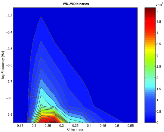
Figure 1: Distribution of detached white-dwarf — white-dwarf binaries in our galaxy as a function of the gravitational wave frequency and chirp mass

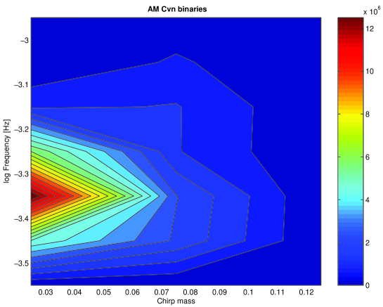
Figure 2: Distribution of AM CVn binary systems in our galaxy as a function of the gravitational wave frequency and chirp mass

4 Numerical Simulation

In order to simulate the LISA $X$ response to the population of WD-WD binaries derived in Section 3 one needs to coherently add the LISA response to each individual signal. Although this could naturally be done in the time domain, the actual CPU time required to successfully perform such a simulation would be unacceptably long. The generation in the time domain of one year of $X^{\rm GW}(t)$ response to a single signal sampled at a rate of $16$ seconds would require about $1$ second with an optimized C++ code running on a Pentium IV $3.2$ GHz processor. Since the number of signals from the background is of the order $10^{8}$, it is clear that a different algorithm is needed for simulating the background in the LISA data within a reasonable amount of time. We were able to derive and implement numerically an analytic formula of the Fourier transform of each binary signal, which has allowed us to reduce the computational time by almost a factor $100$.

We have obtained an approximate analytic expression for the finite-time Fourier transform of each WD-WD signal using the LWL expansion (5) with $n=2$ and by applying the Nuttall’s modified Blackman-Harris window [19] in order to avoid spectral leakage. We have then coherently added in the Fourier domain all the signals radiated by the WD-WD galactic binary population described in section (3). After inverse Fourier transforming the synthesized response and then removing the window from it, we finally obtained the time-domain representation of the background as it will be seen in the LISA TDI combination $X$. This is shown in Figure (3), where we plot three years worth of simulated $X^{\rm GW}(t)$, and include the LISA noise [1]. The one-year periodicity induced by the motion of LISA around the Sun is clearly noticeable. One other interesting feature shown by Figure (3) is that the amplitude response reaches absolute minima when the Sun-LISA direction is roughly oriented towards the Autumn equinox, while the absolute maxima take place when the Sun-LISA direction is oriented roughly towards the Galactic center [5]. This is because the ecliptic plane is not parallel to the galactic plane, and our own solar system is about $8.5\ {\rm kpc}$ away from the galactic center (where most of the of WD-WD binaries are concentrated). As a result it follows that the LISA $X^{\rm GW}$ response to the WD-WD background does not have a six-months periodicity.

Note also that, for a time period of about $2$ months, the absolute minima reached by the amplitude of the LISA response to the WD-WD background is only a factor less than $2$ larger than the level of the instrumental noise. This implies that during these observation times LISA should be able to search for other sources of gravitational radiation that are not located in the galactic plane. This might turn out to be the easiest way to mitigate the detrimental effects of the WD-WD background when searching for other sources of gravitational radiation. We will quantitatively analyze in a follow up work how to take advantage of this observation in order to optimally search, during these time periods, for sources that are off the galactic plane.

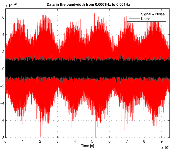
Figure 3: Simulated time series of the WD-WD Galactic background signal of 3 years of data. The time series of LISA instrumental noise is displayed for comparison.

5 Cyclostationary processes

The results of our simulation (Figure 3) indicate that the LISA $X^{\rm GW}$ response to the background can be regarded, in a statistical sense, as a periodic function of time. This is consequence of the deterministic (and periodic) motion of the LISA array around the Sun. Since its autocorrelation function will also be a periodic function of period one year, it follows that any LISA response to the WD-WD background should no longer be treated as a stationary random process but rather as a periodically correlated random process. These kind of processes have been studied for many years, and are usually referred to as cyclostationary random processes (see [20] for a comprehensive overview of the subject and for more references). In what follows we will briefly summarize the properties of cyclostationary processes that are relevant to our problem.

A continuous stochastic process ${\cal X}(t)$ having finite second order moments is said to be cyclostationary with period $T$ if the following expectation values

$$E[{\cal X}(t)] = m(t)=m(t+T),$$ (10)

$$E[{\cal X}(t^{\prime}){\cal X}(t)] = C(t^{\prime},t)=C(t^{\prime}+T,t+T)$$ (11)

are periodic functions of period $T$, for every $(t^{\prime},t)\in{\bf R}\times{\bf R}$. For simplicity from now on we will assume $m(t)=0$.

If ${\cal X}(t)$ is cyclostationary, then the function $B(t,\tau)\equiv C(t+\tau,t)$ for a given $\tau\in{\bf R}$ is periodic with period $T$, and it can be represented by the following Fourier series

$$B(t,\tau)=\sum_{r=-\infty}^{\infty}B_{r}(\tau)e^{i2\pi\frac{rt}{T}}\ ,$$ (12)

where the functions $B_{r}(\tau)$ are given by

$$B_{r}(\tau)=\frac{1}{T}\int^{T}_{0}B(t,\tau)e^{-i2\pi r\frac{t}{T}}\ dt\ .$$ (13)

The Fourier transforms $g_{r}(f)$ of $B_{r}(\tau)$ are the so called “cyclic spectra” of the cyclostationary process ${\cal X}(t)$ [20]

$$g_{r}(f)=\int_{-\infty}^{\infty}B_{r}(\tau)e^{-i2\pi f\tau}\ d\tau\ .$$ (14)

If a cyclostationary process is real, the following relationships between the cyclic spectra hold

$$B_{-r}(\tau) = B^{*}_{r}(\tau)\ ,$$ (15)

$$g_{-r}(-f) = g^{*}_{r}(f)\ ,$$ (16)

where the symbol ^∗ means complex conjugation. This implies that, for a real cyclostationary process, the cyclic spectra with $r\geq 0$ contain all the information needed to characterize the process itself.

The function $\sigma^{2}(\tau)=B(0,\tau)$ is the variance of the cyclostationary process ${\cal X}(t)$, and it can be written as a Fourier decomposition as a consequence of Eq. (13)

$$\sigma^{2}(\tau)=\sum_{r=-\infty}^{\infty}H_{r}e^{i2\pi\frac{r\tau}{T}},$$ (17)

where $H_{r}\equiv B_{r}(0)$ are harmonics of the variance $\sigma^{2}$. From Eq. (15) it follows that $H_{-r}=H^{*}_{r}$.

For a discrete, finite, real time series ${\cal X}_{t}$, $t=1,\ldots,N$ we can estimate the cyclic spectra by generalizing standard methods of spectrum estimation used with stationary processes. Assuming again the mean value of the time series ${\cal X}_{t}$ to be zero, the cyclic autocorrelation sequences are defined as

$$s_{l}^{r}=\frac{1}{N}\sum_{t=1}^{N-|l|}{\cal X}_{t}{\cal X}_{t+|l|}e^{-\frac{i2\pi r(t-1)}{T}}\ .$$ (18)

It has been shown [20] that the cyclic autocorrelations are asymptotically (i.e. for $N\rightarrow\infty$) unbiased estimators of the functions $B_{r}(\tau)$. The Fourier transforms of the cyclic autocorrelation sequences $s_{l}^{r}$ are estimators of the cyclic spectra $g_{r}(f)$. These estimators are asymptotically unbiased, and are called “inconsistent estimators” of the cyclic spectra, i.e. their variances do not tend to zero asymptotically. In the case of Gaussian processes [20] consistent estimators can be obtained by first applying a lag window to the cyclic autocorrelation and then perform a Fourier transform. This procedure represents a generalization of the well-known technique for estimating the spectra of stationary random processes [21].

An alternative procedure for identifying consistent estimators of the cyclic spectra is to first take the Fourier transform, $\tilde{{\cal X}}(f)$, of the time series ${\cal X}(t)$

$$\tilde{{\cal X}}(f)=\sum_{t=1}^{N}{\cal X}_{t}e^{-i2\pi f(t-1)}$$ (19)

and then estimate the cyclic periodograms $g_{r}(f)$

$$g_{r}(f)=\frac{\tilde{{\cal X}}(f)\tilde{{\cal X}}^{*}(f-\frac{2\pi r}{T})}{N}\ .$$ (20)

By finally smoothing the cyclic periodograms, consistent estimators of the spectra $g_{r}(f)$ are then obtained. The estimators of the harmonics $H_{r}$ of the variance $\sigma^{2}$ of a cyclostationary random process can be obtained by first forming a sample variance of the time series ${\cal X}_{t}$. The sample variance is obtained by dividing the time series ${\cal X}_{t}$ into contiguous segments of length $\tau_{0}$ such that $\tau_{0}$ is much smaller than the period $T$ of the cyclostationary process, and by calculating the variance $\sigma^{2}_{I}$ over each segment. Estimators of the harmonics can be obtained by Fourier analyzing the series $\sigma^{2}_{I}$. Note that the definitions of (i) zero order ($r=0$) cyclic autocorrelation, (ii) periodogram, and (iii) zero order harmonic of the variance, coincide with those usually adopted for stationary random processes. Thus, even though a cyclostationary time series is not stationary, ordinary spectral analysis can be used for obtaining the zero order spectrum. Note, however, that cyclostationary random processes provide more spectral information about the time series they are associated with due to the existence of cyclic spectra with $r>0$.

As an important and practical application, let us consider a time series $y_{t}$ consisting of the sum of a stationary random process, $n_{t}$, and a cyclostationary one ${\cal X}_{t}$ (i.e. $y_{t}=n_{t}+{\cal X}_{t}$). Let the variance of the stationary time series be $\nu^{2}$ and its spectral density be $\mathcal{E}(f)$. It is easy to see that the resulting process is also cyclostationary. If the two processes are uncorrelated, then the zero order harmonic $\Sigma^{2}_{0}$ of the variance of the combined processes is equal to

$$\Sigma^{2}_{0}=\nu^{2}+\sigma^{2}_{0}\ ,$$ (21)

and the zero order spectrum $G_{0}(f)$ of $y_{t}$ is

$$G_{0}(f)=\mathcal{E}(f)+g_{0}(f)\ .$$ (22)

The harmonics of the variance as well as the cyclic spectra of $y_{t}$ with $r>0$ coincide instead with those of ${\cal X}_{t}$. In other words, the harmonics of the variance and the cyclic spectra of the process $y_{t}$ with $r>0$ contain information only about the cyclostationary process ${\cal X}_{t}$, and are not “contaminated” by the stationary process $n_{t}$.

6 Data analysis of the background signal

We have numerically implemented the methods outlined in Section 5 and applied them to our simulated WD-WD background signal. A comparison of the results of our simulation of the detached WD-WD background with the calculation of the background by Hils and Bender [10, 15] is shown in Figure 4. Note that in Figure 4 we have given the spectra of the background that do not include LISA instrumental noise. We find that the amplitude of the background from our simulation is a factor of more than $2$ smaller than that of Hils and Bender. The level of the WD-WD background is determined by the number of such systems in the Galaxy. We estimate that our number WD-WD binaries should be correct within a factor $5$ and thus the amplitude of the background should be right within a factor of $\sqrt{5}$. In Figure 4 we have plotted the two backgrounds against the LISA spectral density and we have also included the LISA sensitivity curve. The latter is obtained by dividing the instrumental noise spectral density by the detector GW transfer function averaged over isotropically distributed and randomly polarized signals. In the zero-order long wavelength approximation this averaged transfer function is equal to $\sqrt{3/20}$. Note that for our simulation in the region of the LISA band below $0.2$ millihertz the power of the WD-WD background is smaller than that of the instrumental noise.

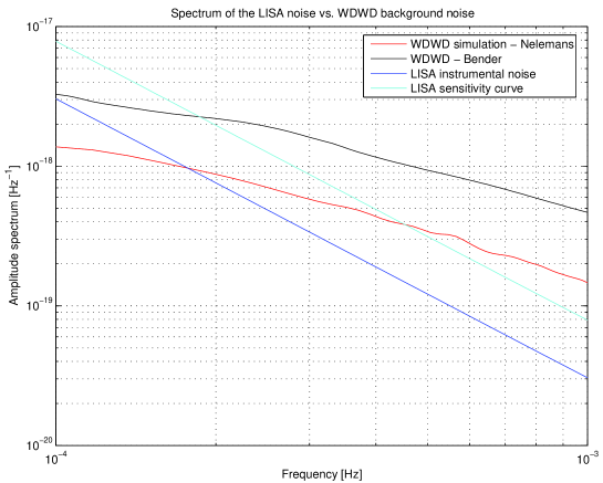
Figure 4: Comparison of detached WD-WD background obtained from binary population synthesis simulation ( [13, 14]) with the WD-WD background calculated by Hils and Bender [10]. Amplitude spectral density of LISA instrumental noise and LISA sensitivity curve are drawn for comparison. All spectral densities are one-sided.

Our analysis was applied to $3$ years of LISA $X$ data consisting of a coherent superposition of signals emitted by detached WD-WD binaries, by semi-detached binaries (AM CVn systems), and of simulated instrumental noise. The noise was numerically generated by using the spectral density of the TDI $X$ observable given in [9]. In addition a $1$ mHz low-pass filter was applied to our data set in order to focus our analysis to the frequency region in which the WD-WD stochastic background is expected to be dominant.

The results of the Fourier analysis of the sample variance of the background signal are shown in Figure 5. The top panel of Figure 5 shows the sample variance of the simulated data for which the variances were estimated over a period of $1$ week; periodicity is clearly visible. The bottom panel instead shows the Fourier analysis of the sample variance for which we have removed the mean from the sample variance time series. The vertical lines correspond to multiples of $1$ year; two harmonics can clearly be distinguished from noise. The other peaks of the spectrum that fall roughly half way between the multiples of $1/{\rm year}$ frequency, are from the rectangular window inherent to the finite time series.

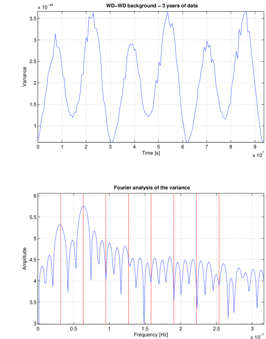
Figure 5: Top panel: sample variance of the simulated WD-WD background. Three years of data are simulated. Data include two populations of the WD-WD binaries, detached and semi-detached ones added to the LISA instrumental noise. The data is passed through a low-pass filter with a cut-off frequency of 1 mHz. Bottom panel: Fourier analysis of the sample variance. Two harmonic are clearly resolved.

In our analysis we have plotted the absolute values $|H_{r}|$ of the coefficients of the Fourier decomposition given by Eq.(17). By using the Fourier transform method, we cannot resolve higher than the second harmonic in our $3$-year data set. We conclude that only the two first harmonics can be extracted reliably from the data.

It is useful to compare the results of our numerical analysis against the analytic calculations of Giampieri and Polnarev [18]. Their analytic expressions for the harmonics of the variance of a background due to binary systems distributed in the galactic disc are given in Eq. (42) and shown in Figure 4 of [18]. Our estimation roughly matches theirs in that the 0th order harmonics is dominant and the first two harmonics have more power than the remaining ones. Our estimate of the power in the second harmonic, however, is larger than that in the first one, whereas they find the opposite. We attribute this difference to their use of a Gaussian distribution of sources in the Galactic disc rather than the (usually assumed) exponential that we adopted. Comparison between these two results suggests that it should be possible to infer the distribution of WD-WD binaries in our Galaxy by properly analyzing the harmonics of the variance of the galactic background measured by LISA. How this can be done will be the subject of a future work.

As a next step in our analysis, we have estimated the cyclic spectra $g_{r}(f)$ (Eq.(14 with $r=1,2,...8$) of the simulated WD-WD background signal. The number $8$ comes from the theoretical predictions of the number of harmonics. The estimated absolute values of the cyclic spectra are shown in Figure 6, where we also plot the spectrum of the LISA instrumental noise and the main spectrum ($r=0$) estimated from the simulation. We find that the main spectrum and the first two cyclic spectra $r=1$ and $r=2$ have the largest magnitude and, over some frequency range, lie above the LISA instrumental noise. The remaining spectra are an order of magnitude smaller and are very noisy. We may also notice that all the cyclic spectra have roughly the same slope. This follows from the assumed independence between the location of the binaries in the Galaxy ($D,\lambda,\beta$) and their frequencies and chirp masses (${\cal M}_{c},\omega_{s}$). We also find the magnitude of the 2nd cyclic spectrum to be higher than the first, similarly to what we had for the harmonics of the variance. Note that we estimated the spectra from the time series consisting of the WD-WD background added to the LISA instrumental noise.

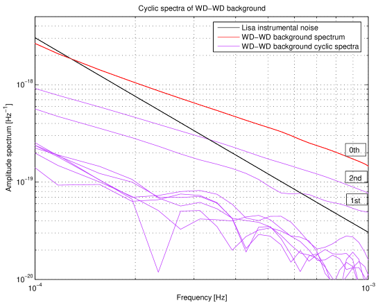
Figure 6: The main (k = 0) spectrum of simulated WD-WD background signal (red). 8 cyclic spectra (magenta) estimated from the simulated data. Spectral density of LISA instrumental noise (black) is shown for comparison. The $0$th order spectrum contains LISA instrumental and hence it differs from the spectrum given in Figure 4.

Our analysis has shown that the LISA data will allow us to compute $17$ independent cyclic spectra (the $8$ complex cyclic spectra $g_{r}(f),r=1,2,...8$ and the real spectrum $g_{0}(f)$) of the WD-WD galactic background, $5$ of which can be expected to be measured reliably. We have also shown that by performing generalized spectral analysis of the LISA data we will be able to derive more information about the WD-WD binary population (properties of the distribution of its parameters) than we would have by only looking at the ordinary $g_{0}(f)$ spectrum.

References

References

- [1] P. L. Bender, K. Danzmann, and the LISA Study Team, Laser Interferometer Space Antenna for the Detection of Gravitational Waves, Pre-Phase A Report, doc. MPQ 233 (Max-Planck-Institüt für Quantenoptik, Garching, 1998).
- [2] M.J. Benacquista, J. DeGoes, and D. Lunder, Class. Quantum Grav., 21, S509, (2004).
- [3] D. Hils, P. L. Bender, and R. F. Webbink, Ap. J., 360, 75 (1900).
- [4] Ch. Evans, Ickp Iben, and L. Smarr, Ap. J., 323, 129 (1987).
- [5] N. Seto, Phys. Rev. D, 69, 123005 (2004).
- [6] A. Królak, M. Tinto, and M. Vallisneri, Phys. Rev. D, 70, 022003 (2004).
- [7] J.A. Edlund, M. Tinto, A. Krolak, and G. Nelemans, In preparation.
- [8] M. Tinto, F.B. Estabrook, and J.W. Armstrong, Phys. Rev. D 65, 082003 (2002).
- [9] F.B. Estabrook, M. Tinto, and J.W. Armstrong, Phys. Rev. D, 62, 042002 (2000).
- [10] D. Hils and P. L. Bender, Ap. J., 360, 75–94 (1990).
- [11] D. Hils and P. L. Bender, Ap. J., 537, 334–341 (2000).
- [12] P. L. Bender and D. Hils, Class. Quantum Grav., 14, 1439–1444 (1997).
- [13] G. Nelemans, L. R. Yungelson, and S. F. Portegies-Zwart, A&A, 375, 890 (2001).
- [14] G. Nelemans, L. R. Yungelson, and S. F. Portegies-Zwart, Mon. Not. Roy. Astron. Soc., 349, 181 (2004).
- [15] Plots and data for Lisa sensitivity curve and WD-WD background due to Hils and Bender can be found on the web page “http://www.srl.caltech.edu/ shane/sensitivity/MakeCurve.html”.
- [16] T. R. Marsh, G. Nelemans, and D. Steeghs, Mon. Not. Roy. Astron. Soc., 350, 113 (2004).
- [17] J. W. Armstrong, F. B. Estabrook, and M. Tinto, Ap. J., 527, 814 (1999).
- [18] G. Giampieri and A. G. Polnarev, Mon. Not. R. Astron. Soc., 291, 149–161 (1997).
- [19] A.H. Nuttal, IEEE Transactions on Acoustics, Speech, and Signal Processing, ASSP-29, 84, (1981).
- [20] H. L. Hurd, IEEE Transactions on Information Theory, 35, 350 (1989).
- [21] D. B. Percival and A. T. Walden, Spectral Analysis for Physical Applications, Cambridge University Press (1993), Chapter 6.