Delocalization of brane gravity by a bulk black hole

Abstract

We investigate the analogue of the Randall-Sundrum brane-world in the case when the bulk contains a black hole. Instead of the static vacuum Minkowski brane of the RS model, we have an Einstein static vacuum brane. We find that the presence of the bulk black hole has a dramatic effect on the gravity that is felt by brane observers. In the RS model, the 5D graviton has a stable localized zero-mode that reproduces 4D gravity on the brane at low energies. With a bulk black hole, there is no such solution — gravity is delocalized by the 5D horizon. However, the brane does support a discrete spectrum of metastable massive bound states, or quasinormal modes, as was recently shown to be the case in the RS scenario. These states should dominate the high frequency component of the bulk gravity wave spectrum on a cosmological brane. We expect our results to generalize to any bulk spacetime containing a Killing horizon.

Introduction

The Randall-Sundrum (RS) model rs consists of a 4D Minkowski brane embedded (with mirror symmetry) in a 5D anti de Sitter (AdS) bulk spacetime. Although the extra dimension is infinite, it is exponentially warped and this leads to the recovery of 4D gravity on the brane at low energies. Thus the RS model provides the basis for models that could describe the observed universe as a brane-world. The key to this feature is the recovery of General Relativity at low energies, i.e., the existence of a normalizable zero-mass mode of the 5D graviton that is a bound state on the brane. General Relativity acquires corrections from the massive modes of the 5D graviton on the brane. (The massive modes dominate over the zero-mode at high energies.)

Why does the RS model allow for a brane-localized zero-mode? The reason is the warp-factor, which erects a potential barrier around the brane that efficiently “squeezes” bulk gravity waves. In this work, we explore the consequences of modifying this barrier by introducing Weyl curvature into the model via a bulk black hole. In order to have a static vacuum configuration, we require a curved brane with an Einstein-static metric. The black hole’s presence has a drastic implication for the zero-mode: there is no longer a gravity-wave bound state solution, because the extreme gravitational field near the horizon causes the brane potential barrier to become highly permeable, or “leaky”.

The bulk metric satisfies the 5D Einstein equations $G^{(5)}_{ab}=-\Lambda_{5}g^{(5)}_{ab}$, and is given by

$$ds^{2}_{(5)} = -f\,dT^{2}+f^{-1}\,dR^{2}+R^{2}\,d\Omega_{(3)}^{2}\,,$$ (1)

$$f = 1-\frac{R_{0}^{2}}{R^{2}}+\frac{R^{2}}{\ell^{2}}=\frac{(R^{2}+R_{\text{h}}^{2}+\ell^{2})(R^{2}-R_{\text{h}}^{2})}{R^{2}\ell^{2}},$$ (2)

where $R_{0}$ determines the ADM mass of the black hole, $\ell$ is the AdS length scale defined by the bulk cosmological constant ($\Lambda_{5}=-6/\ell^{2}$), and

$$R_{\text{h}}^{2}=\frac{\ell^{2}}{2}\left(-1+\sqrt{\frac{4R_{0}^{2}}{\ell^{2}}+1}\right).$$ (3)

Thus, there is an event horizon at $R=R_{\text{h}}$. We define dimensionless coordinates $(t,r)=(T/R_{\text{h}},R/R_{\text{h}})$, so that

$$f(r)=\frac{(r^{2}+\gamma^{2}+1)(r^{2}-1)}{\gamma^{2}r^{2}},\quad\gamma\equiv\frac{\ell}{R_{\text{h}}}.$$ (4)

The bulk geometry is completely characterized by the ratio of the AdS length scale to the black hole horizon radius, $\gamma$, and the horizon is always at $r=1$. It is sensible to call solutions with $\gamma\ll 1$ “big” black holes and solutions with $\gamma\gg 1$ “small” black holes.

A static brane is introduced by identifying $r=r_{\text{b}}$ as the boundary of the bulk and discarding the region $r>r_{\text{b}}$. The brane metric has the Einstein static form,

$$ds^{2}_{(4)}=-d\tau^{2}+R_{\text{h}}^{2}r_{\text{b}}^{2}\,d\Omega_{(3)}^{2}\,,$$ (5)

where $\tau=f_{\text{b}}R_{\text{h}}t=f_{\text{b}}T$ is the cosmic time. In the RS model, the tension (vacuum energy) of the brane exactly cancels the bulk cosmological constant so that the effective 4D cosmological constant vanishes and the brane is Minkowski. Here, the tension exceeds the critical RS value, so that the brane has positive cosmological constant. The acceleration due to this effective cosmological constant is nullified by the “dark radiation” induced by the projection of the bulk Weyl curvature onto the brane. Hence, unlike General Relativity we do not need any additional matter to have an Einstein-static configuration gm . This is a delicate balance, which is why the brane’s position must be fine-tuned.

We can verify this via the junction conditions. The jump in the extrinsic curvature is determined by the energy and stresses on the brane. By the standard junction conditions and the mirror symmetry, the extrinsic curvature of a brane with tension $\sigma$ must satisfy:

$$K_{ab}\equiv g^{c}{}_{b}\nabla^{(5)}_{c}n_{a}=-\frac{\kappa_{5}^{2}}{6}\,\sigma g_{ab}\,,\quad g_{ab}\equiv g^{(5)}_{ab}-n_{a}n_{b}\,,$$ (6)

where $n_{a}=-f^{-1/2}\delta_{a}{}^{R}$ is the normal. Together with Eq. (5), this leads to two equations in the three parameters $\gamma$, $\sigma$, and $r_{b}$, with solutions

$$\sigma(\gamma)=\frac{\gamma^{2}+2}{2\gamma\sqrt{\gamma^{2}+1}},\quad r_{\text{b}}(\gamma)=\frac{\sqrt{2\gamma^{2}+2}}{\gamma}.$$ (7)

The solution for $r_{\text{b}}$ shows that a pure tension brane is coincident with the photon-sphere of the bulk black hole. (This is a special case of the general result that pure tension branes are always totally geodesic for null paths, i.e., they are umbilical surfaces.) Equations (1), (5) and (7) define the Einstein-static (ES) brane-world model.

Tensor perturbations

We now consider tensor perturbations of the bulk metric

$$ds^{2}_{\text{\tiny{($5$)}}}=R_{\text{h}}^{2}[-f\,dt^{2}+f^{-1}\,dr^{2}+r^{2}(h_{ij}+\delta h_{ij})d\theta^{i}d\theta^{j}]\,,$$ (8)

where $h_{ij}d\theta^{i}d\theta^{j}=d\Omega_{(3)}^{2}$. We harmonically decompose the metric perturbation,

$$\delta h_{ij}=\sum_{k}{r^{-3/2}}{\psi_{k}(t,r)}\mathbb{T}^{(k)}_{ij}\,.$$ (9)

The tensor harmonics are defined by

$$\roarrow{\nabla}^{2}\mathbb{T}^{(k)}_{ij}=-k^{2}\mathbb{T}^{(k)}_{ij}\,,\quad\roarrow{\nabla}^{i}\mathbb{T}^{(k)}_{ij}=0=h^{ij}\mathbb{T}^{(k)}_{ij}\,,$$ (10)

where $\roarrow{\nabla}_{i}$ is the covariant derivative of $h_{ij}$ and

$$k^{2}=L(L+2)-2\,,\quad L=1,2,3,\ldots$$ (11)

Using the general results of Kodama and Ishibashi Kodama:2003jz specialized to 5D Schwarzschild-AdS, we see that the linearized Einstein equations show that $\psi_{k}$ satisfies a wave equation,

$$-\frac{\partial^{2}\psi_{k}}{\partial t^{2}} = -\frac{\partial^{2}\psi_{k}}{\partial x^{2}}+V_{k}(r)\psi_{k},\quad x\equiv\int\frac{dr}{f}\,,$$ (12)

$$V_{k}(r) = f\left[\frac{15}{4\gamma^{2}}+\frac{4k^{2}+11}{4r^{2}}+\frac{9(\gamma^{2}+1)}{4\gamma^{2}r^{4}}\right]\!,$$ (13)

where $x$ is the tortoise coordinate and the bulk black hole horizon is at $x=-\infty$. The boundary condition follows from the requirement that the bulk fluctuation preserves the matter content of the brane, i.e., the brane has only tension after perturbation: $\delta K_{ab}=-\kappa_{5}^{2}\sigma\,\delta g_{ab}/6$, which implies

$$\left[\partial_{r}(r^{-3/2}\psi_{k})\right]_{\rm b}=0\,.$$ (14)

It is useful to compare Eq. (12) with the analogous master wave equation in the one-brane RS model:

$$-\frac{\partial^{2}\phi_{k}}{\partial t^{2}} = -\frac{\partial^{2}\phi_{k}}{\partial z^{2}}+U_{k}(z)\phi_{k}\,,$$ (15)

$$\ U_{k}(z) = k^{2}+\frac{15}{4(z-2)^{2}}\,,$$ (16)

where $z$ is a dimensionless conformal coordinate. (For ease of comparison, we are using the mirror image of the bulk on the left of the brane, $z_{\rm b}=1$.) Since the spatial geometry is flat in the RS scenario, $k$ is a continuous parameter. The RS boundary condition is

$$\left[\partial_{z}(z^{-3/2}\phi_{k})\right]_{\rm b}=0\,.$$ (17)

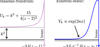
Figure 1: Comparison of the tensor potentials in the Randall-Sundrum and Einstein-static brane-worlds.

The $U_{k}$ and $V_{k}$ potentials are sketched in Fig. 1, where we have added a delta function at the brane position to enforce the boundary condition. The major difference between the two potentials is their asymptotic behaviour far from the branes. In the RS case, the potential decays like $1/z^{2}$ to a positive constant. By contrast, the ES potential decays as ${\rm e}^{2\kappa x}$ for $x\rightarrow-\infty$ (the black hole horizon), where $\kappa$ is the dimensionless surface gravity:

$$\kappa=\frac{1}{2}f^{\prime}(1)=\frac{2+\gamma^{2}}{\gamma^{2}}\,.$$ (18)

Delocalization of the zero-mode

The asymptotic behaviour of the potentials is crucial for the zero-mode. To see this, we assume ${\rm e}^{i\omega t}$ time-dependence for $\psi_{k}$ and $\phi_{k}$, which converts Eqs. (12) and (15) into Schrödinger-type eigenvalue problems with energy parameter $E=\omega^{2}$. From elementary wave mechanics, it is plausible for the RS potential to support a positive-energy normalizable bound state, because there are both an attractive delta function and an asymptotically positive potential. Indeed, such a bound state does exist with $\omega=\pm k$; this is the zero-mode responsible for reproducing General Relativity on the brane. By the same token, the fact that the asymptotic ES potential vanishes strongly means that it cannot support a normalizable bound state with $\omega^{2}>0$. There is no Randall-Sundrum type zero-mode in the Einstein-static brane-world. The vanishing of the potential reflects the fact that the horizon is perfectly transparent to gravity waves, so it is fair to say that the delocalization of brane gravity is entirely due to the bulk black hole.

Is there a tachyonic instability with $\omega^{2}<0$ in the ES brane-world? This cannot be determined from inspection of the potential in Fig. 1. One way to answer this is to conduct ‘scattering experiments’ where the wave equation (12) is solved numerically Seahra:2005wk . As initial data, we choose a Gaussian pulse moving towards the brane at $t=0$. Figure 2 shows a rather clean scattering event where the pulse strikes the brane, is reflected, and then propagates to infinity. At late times, the brane geometry reverts to its background configuration as the fluctuation dies away. This suggests that there is no linear instability in the system, and that none of the energy in the original pulse becomes trapped on the brane. Experimenting with a wide variety of incident signals suggests that both of these conclusions are generic and independent of initial data.

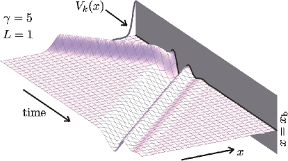
Figure 2: Numerical scattering experiment: a Gaussian gravity wave pulse collides with an Einstein-static brane.

More inferences can be drawn from the late-time gravity wave signals on the brane in these scattering experiments, which are shown in Fig. 3. We consider Gaussian incident pulses with identical characteristics in both the RS and ES (with $k=L=1$) scenarios, and directly compare the resulting waveforms. The RS signal is very well approximated by $\phi_{k}\approx\text{Re}(A{\rm e}^{i\omega t})$, where $A$ is a complex constant. A least-squares fitting gives $\omega=1.00$, which implies that we are seeing stable zero-mode oscillations with $\omega=k$. On the other hand, the ES signal is exponentially damped, in agreement with the behaviour seen in Fig. 2. The waveform is again well-described by $\psi_{k}\approx\text{Re}(A{\rm e}^{i\omega t})$, but with a complex frequency $\omega=0.848+0.256\,i$. Hence as $t\rightarrow\infty$, some of the energy in the incident pulse remains localized on the RS brane while the ES brane radiates it all away. This is a direct numerical confirmation of the claim made above: the brane in the RS scenario supports a stable zero-mode, while the brane in the ES scenario does not.

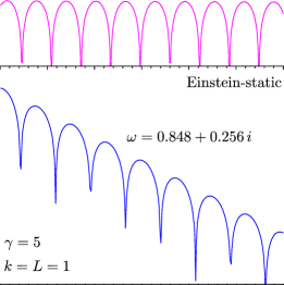
Figure 3: Brane gravity wave signals induced by the scattering of identical Gaussian pulses in the Randall-Sundrum and Einstein-static ($\gamma=5$) scenarios, with $k=1$. The values of $\omega$ are obtained by fitting a $\text{Re}(A{\rm e}^{i\omega t})$ template to each waveform.

Quasinormal modes

The removal of the zero-mode by the bulk black hole is our main result, but the complex-frequency oscillations exhibited in the ES brane-world deserve some investigation. Such behaviour is reminiscent of the familiar ‘ringdown’ waveform from black hole perturbation theory, which is a direct consequence of the existence of so-called ‘quasinormal modes’ (QNMs). These are solutions of the relevant master wave equation subject to purely outgoing boundary conditions, and are characteristic of systems where energy can be lost to infinity. QNMs are described by a discrete set of complex frequencies $\omega_{n}$ with $\text{Im}\,\omega_{n}>0$. Hence, QNMs are exponentially damped in time. These modes are naturally interpreted as metastable bound states or scattering resonances of the potential, i.e., ‘almost trapped’ waves Taylor .

It has recently been demonstrated that the brane in the RS scenario supports QNMs Seahra:2005wk , which are discrete modes embedded within the Kaluza-Klein continuum of massive modes. Thus it is perhaps not surprising that the ES brane exhibits quasinormal ringing. Indeed, one might have expected QNMs from the fact that we are really considering a kind of modified 5D black hole perturbation problem with a boundary. The novel feature is that the ES late-time gravity wave signals are dominated by QNM oscillations. This is in contrast to the RS scenario, where the zero-mode usually obscures the quasinormal ringing. Since these scattering resonances are of crucial importance to actual gravity wave signals, we calculate the QNM spectrum for the ES brane-world.

Our method for finding the QNMs, which is discussed in detail elsewhere other_paper , relies on the series solution of Eq. (12) in the frequency domain. Assuming such a solution satisfies both the brane boundary condition Eq. (14) and the outgoing wave condition,

$$\psi_{k}\sim{\rm e}^{i\omega(t+x)}\text{ as }x\rightarrow-\infty\,,$$ (19)

results in an infinite-order polynomial in $\omega$. Truncation of this polynomial at some order $N$ gives a finite number of complex solutions $\omega^{(N)}_{n}$. Frequencies that are stable in the $N\rightarrow\infty$ limit are the QNM frequencies of the system.

We apply this method to calculate the first eight quasinormal frequencies of the ES brane in the $L=1$ case, as functions of $\gamma$, and the results are plotted in Fig. 4. Frequencies are labelled in order of increasing modulus, the smallest being the fundamental mode ($n=0$) and the others being the overtones ($n=1,\ldots,7$). We can check the validity of the results by examining the value of the fundamental frequency for $\gamma=5$:

$$\omega_{0}=0.8488226912+0.2563765163\,i,$$ (20)

which is in excellent agreement with the best-fit frequency in the bottom panel of Fig. 1.

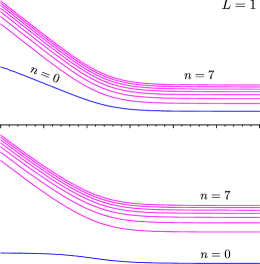
Figure 4: Real (top) and imaginary (bottom) parts of the first eight quasinormal frequencies in the ES brane-world.

Figure 4 shows that the QNM frequencies approach constant values as $\gamma$ becomes large (i.e. for small black holes). This can be understood by examining the leading order behaviour as $\gamma\rightarrow\infty$ of the master equation (12) and boundary condition (14). In this limit, $r\leq r_{\text{b}}\approx\sqrt{2}$, and we can neglect terms of order $r^{2}/\gamma^{2}$. This results in the asymptotic wave equation,

$$-\frac{\partial^{2}\psi_{k}}{\partial t^{2}}=-\left(g\frac{\partial}{\partial r}\right)^{2}\!\psi_{k}+\frac{g[(4k^{2}+11)r^{2}+9]}{4r^{4}}\psi_{k}\,,$$ (21)

where $g(r)=1-1/r^{2}$. The boundary condition reduces to

$$\left[\frac{\partial\psi_{k}}{\partial r}-\frac{3}{2\sqrt{2}}\psi_{k}\right]_{r=\sqrt{2}}=0\,.$$ (22)

Both equations are independent of $\gamma$, and thus the QNM frequencies should also be independent of $\gamma$ in the $\gamma\gg 1$ limit, as confirmed in Fig. 4. We also find that the frequencies are evenly spaced for large $\gamma$, and are well approximated by:

$$\omega_{n}\approx 0.78+0.28\,i+(0.57+1.81\,i)n\,.$$ (23)

The root mean square error between this relationship and the calculated frequencies is 0.02 at $\gamma=100$.

In the small $\gamma$ limit, since $r>1$, we can neglect terms of order $\gamma^{2}/r^{2}$. Writing $\psi_{k}(t,r)={\rm e}^{i\omega t}\Psi_{k}(r)$, the wave equation for $\gamma\ll 1$ is

$$-\gamma^{4}\omega^{2}\Psi_{k}=-\left(h\frac{d}{dr}\right)^{2}\!\Psi_{k}+\frac{h(15r^{4}+9)}{4r^{4}}\Psi_{k}\,,$$ (24)

where $h(r)=(r^{4}-1)/r^{2}$. In this equation, $\gamma^{2}$ and $\omega$ are degenerate because they only appear in the product $\gamma^{2}\omega$. This suggests that the QNM frequencies of the system should obey a power-law scaling $\omega_{n}\propto\gamma^{-2}\approx\kappa$ for $\gamma\ll 1$. This is indeed true for the case of scalar Horowitz:1999jd , electromagnetic, and gravitational Cardoso:2003cj fluctuations of a pure Schwarzschild-AdS black hole with no brane around it. However, the brane boundary condition for $\gamma\ll 1$,

$$\Psi^{\prime}_{k}(r_{\text{b}})=\frac{3\gamma}{2\sqrt{2}}\Psi_{k}(r_{\text{b}})\,,\quad r_{\text{b}}\approx\frac{\sqrt{2}}{\gamma}\,,$$ (25)

breaks the degeneracy, and we should not necessarily expect that $\omega_{n}\propto\gamma^{-2}$ for $\gamma\rightarrow 0$. But in fact, we do see such a scaling for the overtone frequencies in Fig. 4:

$$\omega_{n}\approx\Omega_{n}\gamma^{-2}\text{ for }\gamma\lesssim 0.14\,,\,\,n=1,2,\ldots\,,$$ (26)

where $\Omega_{n}$ is a complex constant determined numerically. For example, by performing a fit between $\gamma=0.10$ and 0.14, we find $\Omega_{1}=3.109+2.814\,i$. The goodness of the fit can be assessed by looking at the RMS discrepancy between the logarithms of the calculated and approximate frequencies. For $n=1$, this error is $10^{-4}$ and $2\times 10^{-3}$ for the real and imaginary parts, respectively.

The small-$\gamma$ behaviour of the fundamental mode is quite different. We find

$$\omega_{0}\approx 1.68\gamma^{-1}+0.497\,i\text{ for }\gamma\lesssim 0.14\,,$$ (27)

i.e., the real part appears to scale like $\gamma^{-1}$ while the imaginary part approaches a constant. The discrepancy in the asymptotic behaviour of the overtones (26) and the fundamental mode (27) would seem to suggest that the latter is more sensitive to the boundary condition.

Attempts to test these relations for much smaller values of $\gamma$ are constrained by computing speed, since for $\gamma\rightarrow 0$, we have $r_{\text{b}}\rightarrow\infty$, which is a singular point of the master wave equation (12) in the frequency domain. Hence the series solution for $\psi_{k}$ becomes poorly convergent at the brane, which means we must retain unreasonably many terms to get accurate QNM frequencies.

We have also calculated QNM frequencies for different values of $L$, i.e., for perturbations on different spatial scales on the brane. The results for $\gamma=5$ are shown in Fig. 5. The general trend is that the real parts of the frequencies increase with $L$ (i.e., for smaller scales), while the imaginary parts remain roughly constant or decrease slightly. This is in keeping with results obtained for the scalar QNMs of a 4D Schwarzschild-AdS black hole with no brane Horowitz:1999jd .

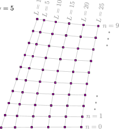
Figure 5: The first ten quasinormal frequencies of the $\gamma=5$ ES brane for various values of $L$.

Kaluza-Klein masses?

In the RS scenario, the various modes of the 5D graviton can be labelled by an effective 4D Kaluza-Klein (KK) mass. This can be understood as follows: The RS potential in (15) can be re-written as

$$U_{k}(z)=k^{2}+\overline{U}(z)\,,$$ (28)

where $\overline{U}$ is independent of the spatial scale $k$. With $\phi_{k}(t,z)={\rm e}^{i\omega t}\varphi_{k}(z)$, we find the dispersion relation

$$m^{2}=E^{2}-p^{2},\quad E=\omega/\ell,\quad p=k/\ell\,,$$ (29)

where $m^{2}\ell^{2}$ is the eigenvalue of $-(d/dz)^{2}+\overline{U}(z)$. To a stationary brane observer, $E$ is the energy of the mode while $p$ is its 3-momentum. Hence, $m=\sqrt{E^{2}-p^{2}}$ is naturally interpreted as the effective 4D graviton mass according to the standard KK paradigm.

By contrast, in the ES brane-world, the spatial scale $k$ can no longer be separated from the potential $V_{k}$, and no simple position-independent dispersion relation like (29) can be found. At best, we can define a local dispersion relation on the brane:

$$\tilde{m}^{2}=\tilde{E}^{2}-\tilde{p}^{2},\quad\tilde{E}=\frac{\omega}{R_{\text{h}}\sqrt{f_{\text{b}}}},\quad\tilde{p}=\frac{k}{R_{\text{h}}r_{\text{b}}}\,.$$ (30)

Note that in the shortwave approximation $k\gg 1$, $\tilde{E}$ and $\tilde{p}$ are the mode’s energy and 3-momentum as measured by comoving brane observers, respectively, and $\tilde{m}$ is the effective mass of the mode.

What are the masses of the QNMs we calculated above? We continue (30) into the complex plane in order to define a complex mass for each QNM. Then, $\text{Re}\,\tilde{m}_{n}$ is interpreted as the conventional mass of the resonance, while $(\text{Im}\,\tilde{m}_{n})^{-1}$ is roughly its half-life. Our results for $\tilde{m}_{n}$ for $L=80$ are shown in Fig. 6. Interestingly, the upper panel suggests a mass gap between the fundamental mode and the overtones for small $\gamma$, i.e., for large black hole effects. This is reminiscent of a de Sitter brane-world Garriga:1999bq (although in the de Sitter case, the gap is between the zero-mode and the KK continuum).

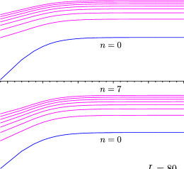
Figure 6: Effective 4D masses, as measured by brane observers, of the first eight QNMs in the $L=80$ case

Generalizations

One can generalize the ES brane-world model by making the bulk more complicated, letting the brane move, or both. Will our results carry over to these new situations?

First consider the addition of matter fields in the bulk. These may take the form of dilatons, moduli fields, supergravity form fields, etc. Stationary, spherically symmetric solutions sourced by such matter and featuring an event horizon are classified as “dirty black holes”. Scalar wave propagation in 4D dirty black hole spacetimes shows Medved:2003rg that the potential in the master wave equation vanishes at the horizon, just as in Eq. (12). Now, the key reason that the zero-mode becomes delocalized in the ES model is the fact that $V(R_{\text{h}})=0$. Hence, if we make the natural assumption that the behaviour seen in Ref. Medved:2003rg generalizes to spin-2 fields and higher-dimensional backgrounds, we conclude that the zero-mode will remain delocalized if the 5D Schwarzschild-AdS bulk is replaced with a dirty black hole. Indeed, we can go even further by conjecturing that any static brane located outside a stationary Killing horizon cannot support a normalizable zero-mode, precisely because any such horizon be will completely transparent to bulk gravity waves.

Next, consider brane motion in a Schwarzschild-AdS bulk, $r_{\text{b}}=r_{\text{b}}(t)$ as in model of brane cosmology. Do the QNM frequencies we have calculated tell us anything about the behaviour of cosmological perturbations? Fluctuations with $|\omega|\gg H\equiv\dot{r}_{\text{b}}/r_{\text{b}}$ do not ‘feel’ the expansion of the universe and effectively ‘see’ the brane as stationary, i.e., the characteristic timescale of the perturbation is much larger than the characteristic timescale of the cosmological dynamics. Hence, we can expect the QNMs calculated for a static brane to be approximate solutions for the gravity waves around a moving brane if $1/|\omega_{n}|$ is much shorter than the Hubble time. Such QNMs will dominate that part of the bulk gravity wave spectrum. Hence, the high frequency $\omega\gg H$ component of the bulk gravity wave spectrum on a cosmological brane should be dominated by the metastable bound state resonances of the corresponding static brane.

Such an approximation has the potential to greatly simplify the thorny problem of brane cosmological perturbations, but there is a significant caveat. The QNMs we have calculated are only for one brane position, i.e., on the photon sphere. In order to have a complete picture, we need to know the QNM frequencies for static branes over a range in $r$, corresponding to the addition of matter on the ES brane. The calculation of these frequencies is the subject of a separate paper other_paper .

Conclusions

We have considered static pure-tension branes surrounding a 5D bulk black hole. By studying the tensor perturbations, we have seen that the bulk Killing horizon causes the brane’s zero-mode to become delocalized. In other words, the gravitational field of the black hole makes it impossible for the brane to support a normalizable bound state. However, we also found that the brane supports a discrete spectrum of metastable bound states, or quasinormal modes, as in the Randall-Sundrum scenario. Using a series solution of the master wave equation, we have calculated the quasinormal frequency spectrum. We discussed why the massive mode Kaluza-Klein decomposition common in other brane-world models does not work in the current problem, but then showed how one could define an effective local mass measured by brane observers. The locally defined mass shows a gap between the fundamental and overtone modes.

Our results are expected to generalize in several important ways. We expect that whenever there is a stationary Killing horizon in the bulk, a surrounding brane cannot support a normalizable bound state. Furthermore, we expect that the high frequency bulk gravity wave spectrum on a moving brane will be well represented by a sum over the quasinormal resonances of the corresponding static brane.

References

- (1) L. Randall and R. Sundrum, Phys. Rev. Lett. 83, 4690 (1999) [arXiv:hep-th/9906064].
- (2) L. Gergely and R. Maartens, Class. Quant. Grav. 19, 213 (2002) [arXiv:gr-qc/0105058].
- (3) H. Kodama and A. Ishibashi, Prog. Theor. Phys. 110, 701 (2003) [arXiv:hep-th/0305147].
- (4) I. Tanaka and H. Ishihara, in Proceedings of the 13th Workshop on General Relativity & Gravitation in Japan, 260 (2003).
- (5) S. S. Seahra, arXiv:hep-th/0501175.
- (6) J. R. Taylor, Scattering Theory (New York, Wiley, 1972).
- (7) C. Clarkson and S. S. Seahra, in preparation.
- (8) G. T. Horowitz and V. E. Hubeny, Phys. Rev. D62, 024027 (2000) [arXiv:hep-th/9909056].
- (9) V. Cardoso, R. Konoplya and J. P. S. Lemos, Phys. Rev. D68, 044024 (2003) [arXiv:gr-qc/0305037].
- (10) J. Garriga and M. Sasaki, Phys. Rev. D62, 043523 (2000) [arXiv:hep-th/9912118]; D. Langlois, R. Maartens and D. Wands, Phys. Lett. B489, 259 (2000) [arXiv:hep-th/0006007].
- (11) A. J. M. Medved, D. Martin, and M. Visser, Class. Quant. Grav. 21, 1393 (2004) [arXiv:gr-qc/0310009].