LISA source confusion: identification and characterization of signals

Abstract

The Laser Interferometer Space Antenna (LISA) is expected to detect gravitational radiation from a large number of compact binary systems. We present a method by which these signals can be identified and have their parameters estimated. Our approach uses Bayesian inference, specifically the application of a Markov chain Monte Carlo method. The simulation study that we present here considers a large number of sinusoidal signals in noise, and our method estimates the number of periodic signals present in the data, the parameters for these signals and the noise level. The method is significantly better than classical spectral techniques at performing these tasks and does not use stopping criteria for estimating the number of signals present.

1 Introduction

LISA [1] is expected to detect a very large number of signals from compact binaries in the $10^{-2}$ mHz to $100$ mHz band, making signal identification very difficult. Tens of thousands of signals could be present in the data with significant signal-to-noise ratios. In the 0.1 mHz to 3 mHz band there will be numerous signals from white dwarf binaries. Sources above 5 mHz should be resolvable, however below 1 mHz there will be source confusion. In the 1 mHz to 5 mHz band we expect as many as $10^{5}$ potential sources [2, 3, 4] resulting in an astoundingly difficult data analysis problem. We direct the reader to Barack & Cutler [2] and Nelemans et al. [5] for an in-depth description of the population of binary systems in the LISA operating band, and how LISA’s performance is influenced by them.

The goal of this paper is to introduce the LISA data analysis community to a new approach for identifying and characterizing these numerous signals. We apply Bayesian Markov chain Monte Carlo (MCMC) methods to a simplified problem that will serve as an example of the technique. MCMC methods are a numerical means of parameter estimation, and are especially useful when there are a large number of parameters [6]. We have already applied MCMC methods to other gravitational radiation parameter estimation problems; for example, we have used a Metropolis-Hastings (MH) algorithm [7, 8] for estimating astrophysical parameters for gravitational wave signals from coalescing compact binary systems [9], and pulsars [10, 11]. We believe that MCMC methods could provide an effective means for identifying sources in LISA data. We summarize our reversible jump MCMC technique in this paper. A more detailed and comprehensive description can be found in [12].

Here we present a summary of our study of some simple simulated data, comprising a number of sinusoidal signals embedded in noise. Our reversible jump MCMC algorithm infers the parameters for each (sufficiently large) sinusoidal signal, the magnitude of the noise and the number of signals present. In our approach we solve both the detection and parameter estimation problems without the need for evaluating formal model selection criteria. The method does not require a stopping criterion for determining the number of signals and produces results which compare very favorably with classical spectral techniques. A Bayesian analysis naturally encompasses Occam’s Razor and a preference for a simpler model [13]. In addition, our MCMC method is better than a classical periodogram at resolving signals that are very close in frequency, and we provide an explanation of how to identify these signals.

The method that we present here is not a source subtraction method [14]. Signals that are sufficiently strong will be identified with a quoted confidence, and sources that are weak will simply contribute to the noise, the level of which we also estimate. We show that the noise level estimate from our method depends (as it should) on the inherent detector noise level, and also the presence of unidentified signals. A benefit of using MCMC methods is that computation time does not show an exponential increase with the number of parameters [6].

The problem of identifying an unknown number of sinusoids is neither new nor simple [15, 16]. Previous studies have looked for a handful of unknown signals, here we show results for 100 signals. MCMC methods are robust and dynamic, and we believe that ultimately it will be possible to use them with LISA data to estimate the parameters of all modelled sources types. In the future we will make the model more complex, taking into account the orbit of the LISA spacecraft and binary source evolution.

2 Occam factors

One can approach the problem of identifying and enumerating sinusoidal signals in noise from a number of different directions, but one thing is clear. Discrete noisy data can be fitted exactly if one uses a sufficient number of components – the result is simply the discrete Fourier transform of the data. Classically, we proceed by estimating the noise floor of the spectrum and identify a threshold spectral power that divides the components between signals and noise. In this way we prevent the model from overfitting the noise. In an iterative fitting procedure, this is achieved by halting when the statistics of the residuals fit the noise model well. One very attractive, and well known, feature of Bayesian inference is that these ideas are within the fabric of the method. Indeed they are such a basic property of logical inference that there is no need to refer to ideas such as ‘overfitting’ at all. More generally, the method discourages us from using models that have more degrees of freedom than are necessary for the problem in hand.

One can see how this works in a simple example: Take two data models, $\mathcal{M}_{1}$ and $\mathcal{M}_{2}$ constrained by a single datum, $d$. $\mathcal{M}_{1}$ has one parameter, $a_{1}$, to describe the datum, whereas $\mathcal{M}_{2}$ uses the sum of two parameters, $s=a_{1}+a_{2}$ to describe the same datum. Which model is better? Here we have no noise and no random variables, so this is not a problem for orthodox statistics. However, if the datum is equally consistent with both models, we would clearly prefer the simpler model $\mathcal{M}_{1}$ in favour of $\mathcal{M}_{2}$.

Within the Bayesian framework we consider the odds ratio of the two models:

$$\mathcal{O}_{12}=\frac{p(\mathcal{M}_{1}|d)}{p(\mathcal{M}_{2}|d)}=\frac{p(\mathcal{M}_{1})}{p(\mathcal{M}_{2})}\frac{p(d|\mathcal{M}_{1})}{p(d|\mathcal{M}_{2})}.$$ (1)

We will set $p(\mathcal{M}_{1})/p(\mathcal{M}_{2})$ to unity, as we have no prior preference for either model, and take the priors for $a_{1}$ and $a_{2}$ to be each uniform in the range $0\rightarrow R$, making the prior for $s$ the convolution of two of these. The functional priors for $a_{1}$ under $\mathcal{M}_{1}$ and $s$ under $\mathcal{M}_{2}$ are therefore

$$p(a_{1}|\mathcal{M}_{1})=\frac{1}{R};\qquad p(s|\mathcal{M}_{2})=\cases{s/R^{2}&\kern-20.00003ptfor $0<s<R$\\ 2/R-s/R^{2}&\kern-20.00003ptfor $R<s<2R$.}$$ (2)

The probability of the data, given either model, is simply a Dirac delta function centred on the value of the datum, so we can calculate the evidences $p(d|\mathcal{M}_{1})$ and $p(d|\mathcal{M}_{2})$ by marginalising over the allowed parameter values:

$$p(d|\mathcal{M}_{1})=\int_{0}^{R}\frac{1}{R}\delta(d-a_{1})\,\,{\rm d}a_{1}=\cases{1/R&\kern-20.00003ptfor $0<d<R$\\ 0&\kern-20.00003ptotherwise,}$$ (3)

$$p(d|\mathcal{M}_{2})=\int_{0}^{2R}p(s|\mathcal{M}_{2})\delta(d-s)\,\,{\rm d}s=\cases{d/R^{2}&\kern-20.00003ptfor $0<d<R$\\ 2/R-d/R^{2}&\kern-20.00003ptfor $R<d<2R$\\ 0&\kern-20.00003ptotherwise.}$$ (4)

as shown in Fig. 1.

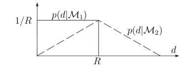
Figure 1: The evidences for models $\mathcal{M}_{1}$ (solid line, one parameter fit) and $\mathcal{M}_{2}$ (dashed line, two parameter fit) as a function of the datum $d$. Note that the evidence ratio always favours the simpler model $\mathcal{M}_{1}$ when the datum is equally consistent with either.

If the datum lies in the range $0<d<R$, the odds ratio is $(1/R)/(d/R^{2})=R/d$, so that $\mathcal{M}_{1}$ will always favoured over $\mathcal{M}_{2}$ in that range. If $d=R$ the odds ratio is unity, and if $R<d<2R$ the only possible model is $\mathcal{M}_{2}$.

This demonstrates why the simpler model is favoured even when the datum is equally consistent with both: $\mathcal{M}_{2}$ has more flexibility than is necessary to explain the datum and so penalizes itself by spreading its evidence more thinly.

Although in this example we consider a probability ratio to determine our favoured model, when more than two models are available we can consider the model choice to be a parameter itself, and determine its marginal posterior probability in the usual way.

A slightly more pertinent, though still highly restricted, example would be a data set $\{d_{k}\}$ that consists of observations of the sum of $m$ sinusoids of the form $A_{i}\sin(2\pi f_{i}t)$ at times $t=t_{k}$ and Gaussian noise with variance $\sigma^{2}$. We also know that $0\leq m\leq 5$, and $A_{i}$ and $f_{i}$ can only take the discrete values $A_{i}\in\{1,\ldots,5\}$ and $f_{i}\in\{0.01,0.02,\ldots,0.05\}$.

For this discrete problem, assuming uniform priors on $m$, $A_{i}$ and $f_{i}$ for each sinusoid, we can identify the probability of any particular $m$, given the data, irrespective of the other signal parameters:

$$p(m|\{d_{k}\})\propto\frac{1}{25^{m}}\sum_{A_{1},f_{1}}\ldots\sum_{A_{M},f_{M}}\exp(-\chi^{2}/2)$$ (5)

where

$$\chi^{2}=\frac{1}{\sigma^{2}}\sum_{k}\left[d_{k}-\sum_{i=1}^{m}A_{i}\sin(2\pi f_{i}t_{k})\right]^{2}.$$ (6)

Here it is the factor of $25^{m}$, originating from the $m$ normalised priors for the model parameters, that offsets the increasingly good $\chi^{2}$ fit that might come from large values of $m$ and provides our Occam factor.

This discrete problem can be solved by directly marginalising over the nuisance amplitude and frequency parameters. However problems with more and/or with continuous parameters are not approachable using such direct methods, and must be tackled in another way.

3 Parameter estimation

We consider the continuous case as a signal consisting of $m$ superimposed sinusoids where $m$ is unknown. Therefore we confine our attention to a set of models $\{\mathcal{M}_{m}:m\in\{1,\cdots,M\}\}$ where $M$ is the maximum allowable number of sinusoids. Let $\mbox{\boldmath$d$}=[d_{1},\cdots,d_{N}]$ be a vector of $N$ samples recorded at times $\mbox{\boldmath$t$}=[t_{1},\cdots,t_{N}]$. Model $\mathcal{M}_{m}$ assumes that the observed data are composed of a signal plus noise: $d_{j}=\mathrm{f}_{m}(t_{j},\mbox{\boldmath$a$}_{m})+\epsilon_{j}$, for $j=1\ldots N$, where the noise terms $\epsilon_{j}$ are assumed to be i.i.d. $N(0,\sigma_{m}^{2})$ random variables. The signal of model $\mathcal{M}_{m}$ is assumed to be of the form

$$\mathrm{f}_{m}(t_{j},\mbox{\boldmath$a$}_{m})=\sum_{i=1}^{m}{\left[A_{i}^{(m)}\cos(2\pi f_{i}^{(m)}t_{j})+B_{i}^{(m)}\sin(2\pi f_{i}^{(m)}t_{j})\right]}.$$ (7)

Model $\mathcal{M}_{m}$ is therefore characterized by a vector

$$\mbox{\boldmath$a$}_{m}=[A_{1}^{(m)},B_{1}^{(m)},f_{1}^{(m)},\cdots,A_{m}^{(m)},B_{m}^{(m)},f_{m}^{(m)},\sigma^{2}_{m}]$$ (8)

of $3m+1$ unknown parameters. The objective is to find the model $\mathcal{M}_{m}$ that best fits the data. To this end, we use a Bayesian approach as in [17]. The joint probability of these data $d$ given the parameter vector $\mbox{\boldmath$a$}_{m}$ and model $\mathcal{M}_{m}$ is

$$p(\mbox{\boldmath$d$}|m,\mbox{\boldmath$a$}_{m})\propto\frac{1}{\sigma^{N}_{m}}\exp\left\{-\frac{1}{2\sigma^{2}_{m}}\sum_{j=1}^{N}\left[d_{j}-\mathrm{f}_{m}(t_{j},\mbox{\boldmath$a$}_{m})\right]^{2}\right\}.$$ (9)

We choose (now continuous) uniform priors for the amplitudes $A_{i}^{(m)}$,$B_{i}^{(m)}$ and frequency $f_{i}^{(m)}$ with ranges $A_{i}^{(m)}\in[-A_{\rm max},A_{\rm max}]$, $B_{i}^{(m)}\in[-B_{\rm max},B_{\rm max}]$ and $f_{i}^{(m)}\in[0,0.5]$, respectively. Furthermore we use a uniform prior for $m$ over $\{1,\ldots,M\}$ and vague inverse Gamma priors for $\sigma_{m}^{2}$. By applying Bayes’ theorem, we obtain the posterior pdf

$$p(m,\mbox{\boldmath$a$}_{m}|\mbox{\boldmath$d$})=\frac{p(m,\mbox{\boldmath$a$}_{m})p(\mbox{\boldmath$d$}|m,\mbox{\boldmath$a$}_{m})}{p(\mbox{\boldmath$d$})},$$ (10)

where $p(\mbox{\boldmath$d$})=\sum_{i=1}^{M}\int p(m,\mbox{\boldmath$a$}_{m})p(\mbox{\boldmath$d$}|m,\mbox{\boldmath$a$}_{m})\,\,{\rm d}\mbox{\boldmath$a$}_{m}$. We use a sampling-based technique for posterior inference via MCMC [6]. MCMC techniques only require the unnormalised posterior $p(m,\mbox{\boldmath$a$}_{m}|\mbox{\boldmath$d$})\propto p(m,\mbox{\boldmath$a$}_{m})p(\mbox{\boldmath$d$}|m,\mbox{\boldmath$a$}_{m})$ to simulate from Eq. (10) in order to estimate the quantities of interest. However, as the dynamic variable of the simulation does not have fixed dimension, the classical MH techniques [7, 8] cannot be adopted when proposing trans-dimensional moves between models where the model indicator $m$ determines the dimension ($3m+1$) of the parameter vector $\mbox{\boldmath$a$}_{m}$. We therefore use the Reversible Jump Markov Chain Monte Carlo (RJMCMC) algorithm [18, 19] for model determination, as in [16]. For transitions within the same model, we use the delayed rejection method [20, 21] which yields a better adaptation of the proposals in different parts of the state space.

3.1 The RJMCMC for model determination

To sample from the joint posterior $p(m,\mbox{\boldmath$a$}_{m}|\mbox{\boldmath$d$})$ via MCMC, we need to construct a Markov chain simulation with state space $\displaystyle\cup_{m=1}^{M}\left({m}\times I\!\!R^{3m+1}\right)$. When a new model is proposed we attempt a step between state spaces of different dimensionality. Suppose that at the $n$th iteration of the Markov chain we are in state $(k,\mbox{\boldmath$a$}_{k})$. If model $\mathcal{M}_{k^{\prime}}$ with parameter vector $\mbox{\boldmath$a$}_{k^{\prime}}^{\prime}$ is proposed, a reversible move has to be considered in order to preserve the detailed balance equations of the Markov chain. Therefore the dimensions of the models have to be matched by involving a random vector $r$ sampled from a proposal distribution with pdf $q$, say, for proposing the new parameters $\mbox{\boldmath$a$}_{k^{\prime}}^{\prime}=\textrm{t}(\mbox{\boldmath$a$}_{k},\mbox{\boldmath$r$})$ where t is a suitable deterministic function of the current state and the random numbers. Here we focus on transitions that either decrease or increase models by one signal, i.e. $k^{\prime}\in\{k-1,k+1\}$. We use equal probabilities $p_{k\mapsto k^{\prime}}=p_{{k^{\prime}\mapsto k}}$ to either move up or down in dimensionality. Without loss of generality, we consider $k<k^{\prime}$.

If the transformation $\textrm{t}_{k\mapsto k^{\prime}}$ from $(\mbox{\boldmath$a$}_{k},\mbox{\boldmath$r$})$ to $\mbox{\boldmath$a$}_{k^{\prime}}^{\prime}$ and its inverse $\textrm{t}_{k\mapsto k^{\prime}}^{-1}=\textrm{t}_{k^{\prime}\mapsto k}$ are both differentiable, then reversibility is guaranteed by defining the acceptance probability for increasing a model by one signal according to [18] by

$$\alpha_{k\mapsto k^{\prime}}(\mbox{\boldmath$a$}_{k^{\prime}}^{\prime}|\mbox{\boldmath$a$}_{k})=\min\left\{1,\frac{p(\mbox{\boldmath$a$}_{k^{\prime}}^{\prime},k^{\prime})p(\mbox{\boldmath$d$}|\mbox{\boldmath$a$}^{\prime}_{k^{\prime}},k^{\prime})p_{k\mapsto k^{\prime}}}{p(\mbox{\boldmath$a$}_{k},k)p(\mbox{\boldmath$d$}|\mbox{\boldmath$a$}_{k},k)q(\mbox{\boldmath$r$})p_{k^{\prime}\mapsto k}}\right\}\left|J_{k\mapsto k^{\prime}}\right|$$ (11)

where $|J_{k\mapsto k^{\prime}}|=\left|\frac{\partial\textrm{t}(\mbox{\boldmath$a$}_{k},\mbox{\boldmath$r$})}{\partial(\mbox{\boldmath$a$}_{k},\mbox{\boldmath$r$})}\right|$ is the Jacobian determinant of this transformation and $q(\mbox{\boldmath$r$})$ is the proposal distribution.

In this context, two types of transformations, ‘split-and-merge’ and ‘birth-and-death’, are obvious choices. In a ‘split-and-merge’ transition, the proposed parameter vector $\mbox{\boldmath$a$}^{\prime}_{k^{\prime}}$ comprises all $(k-1)$ subvectors of $\mbox{\boldmath$a$}_{k}$ except a randomly chosen subvector $\mbox{\boldmath$a$}_{(i)}=(A_{i}^{(k)},B_{i}^{(k)},f_{i}^{(k)})^{\prime}$ which is replaced by two 3-dimensional subvectors,

$$\mbox{\boldmath$a$}_{(i_{1})}^{\prime}=\left(A_{i_{1}}^{(k^{\prime})},B_{i_{1}}^{(k^{\prime})},f_{i_{1}}^{(k^{\prime})}\right)\quad{\rm and}\quad\mbox{\boldmath$a$}_{(i_{2})}^{\prime}=\left(A_{i_{2}}^{(k^{\prime})},B_{i_{2}}^{(k^{\prime})},f_{i_{2}}^{(k^{\prime})}\right)$$

with roughly half the amplitudes but about the same frequency as $\mbox{\boldmath$a$}_{(i)}$.

A three-dimensional Gaussian random vector (with mean zero), $\mbox{\boldmath$r$}=(r_{A},r_{B},r_{f})$, changes the current state $\mbox{\boldmath$a$}_{(i)}$ to the two resulting states $\mbox{\boldmath$a$}_{(1i)}^{\prime},\mbox{\boldmath$a$}_{(2i)}^{\prime}$ through a linear transformation

$$\textrm{t}_{k\mapsto k^{\prime}}(\mbox{\boldmath$a$}_{(i)},\mbox{\boldmath$r$})=\left(\frac{1}{2}A_{i}^{(k)}\!+r_{A},\frac{1}{2}B_{i}^{(k)}\!+r_{B},f_{i}^{(k)}\!+r_{f},\frac{1}{2}A_{i}^{(k)}\!-r_{A},\frac{1}{2}B_{i}^{(k)}\!-r_{B},f_{i}^{(k)}\!-r_{f}\right)$$

$$\phantom{\textrm{t}_{k\mapsto k^{\prime}}(\mbox{\boldmath$a$}_{(i)},\mbox{\boldmath$r$})}=\left(A_{i_{1}}^{(k^{\prime})},B_{i_{1}}^{(k^{\prime})},f_{i_{1}}^{(k^{\prime})},A_{i_{2}}^{(k^{\prime})},B_{i_{2}}^{(k^{\prime})},f_{i_{2}}^{(k^{\prime})}\right).$$ (12)

By analogy, the inverse transformation $\textrm{t}^{-1}_{k\mapsto k^{\prime}}:=\textrm{t}_{k^{\prime}\mapsto k}$ accounts for the merger of two signals. Note that the determinant of the Jacobian of the transformation $\textrm{t}_{k\mapsto k^{\prime}}$ is $|J_{k\mapsto k^{\prime}}|=2$, and that of its inverse is 1/2.

We use a multivariate normal distribution, $N[\textbf{0},\textrm{diag}(\sigma_{A}^{2},\sigma_{B}^{2},\sigma_{f}^{2})]$, for the proposal distribution $q(\mbox{\boldmath$r$})$. Care has to be taken in choosing suitable values for the proposal variances to achieve reasonable acceptance probabilities in Eq. (11).

The second ‘birth-and-death’ transformation consists of the creation of a new signal with parameter triple $\mbox{\boldmath$a$}_{(i)}^{\prime}$ independent of other existing signals in the current model $\mathcal{M}_{k}$. The one-to-one transformation in this case is very simply given by $\textrm{t}_{k\mapsto k^{\prime}}(\mbox{\boldmath$r$})=\mbox{\boldmath$r$}=\mbox{\boldmath$a$}_{(k+1)}^{\prime}$ with Jacobian equal to 1.

Here, $q$ is the three-dimensional pdf from which we draw proposals for the additional signal. We use independent uniform distributions with frequency range $0\leq f\leq 0.5$ and amplitude range $(A_{i}^{2}+B_{i}^{2})^{1/2}<l_{A}$ where $l_{A}$ is the radius for the two amplitudes of the signal in polar coordinates. Again, the radii of the uniform proposal densities have to be tuned to achieve an optimal acceptance rate.

3.2 The delayed rejection method for parameter estimation

For transitions within a model $\mathcal{M}_{m}$, classical MCMC methods can be applied. Here, however, we use an adaptive MCMC technique, the delayed rejection method  [20, 21, 22] that we have successfully applied to estimate parameters of pulsars [11]. The idea behind the delayed rejection method is that persistent rejection indicates that locally, the proposal distribution is badly calibrated to the target. Therefore, the MH algorithm is modified so that on rejection, a second attempt to move is made with a proposal distribution that depends on the previously rejected state. In this context, when a proposed MH move is rejected from a bold normal distribution with large variance a second candidate can be proposed with a timid proposal distribution for sampling the parameters for the individual sinusoids. Hence, the main objective of the first stage is a coarse scan of the parameter space and therefore we choose the variances of the parameters about one order of magnitude smaller than the prior ranges of the corresponding parameters. Once a mode is found, we aim to draw representative samples in the second stage.

The precision of the frequency in a single-frequency model depends on the amplitude, the variance $\sigma^{2}$ of the noise, and the number of samples $N$ of the data set [17, 23]. The precision of the frequency has been derived in [17] by a Gaussian approximation to the posterior pdf of the frequency and calculation of its standard deviation, given by $\sigma_{f}^{\prime\prime}=(2\pi)^{-1}[48\sigma^{2}/N^{3}(A^{2}+B^{2})]^{1/2}$. We therefore choose proposals with this standard deviation.

3.3 Starting values

The starting values of a Markov chain are crucial for the length of the burn-in period, i.e. the time needed for the chain to achieve convergence to the real posterior distribution. We perform a Fast Fourier Transformation (FFT) prior to the simulation and use corresponding estimates as starting values. Arthur Schuster introduced the periodogram [24]

$$C(f)=\frac{1}{N}\left[R(f)^{2}+I(f)^{2}\right]$$ (13)

where $R(f)=\sum_{j=1}^{N}{d_{j}\cos\left(2\pi ft_{j}\right)}$ and $I(f)=\sum_{j=1}^{N}{d_{j}\sin\left(2\pi ft_{j}\right)}$ are the real and imaginary parts from the sums of the discrete Fourier transformation. As a starting value for $m$, we use the number $m_{0}$ of local maxima in the periodogram that exceed a certain noise level (lower than the expected one). We use the frequencies corresponding to the local maxima in the periodogram, $f_{0,i}$, as starting values for $f_{0,i}^{(m_{0})}$ and $A_{0,i}=2R(f_{0,i})/N$, $B_{0,i}=2I(f_{0,i})/N$ as starting values for $A_{i}^{(m_{0})}$ and $B_{i}^{(m_{0})}$, respectively.

3.4 Identifying the sinusoids

Although the RJMCMC offers great ease in model selection, we still encounter the label-switching problem, a general problem due to invariance of the likelihood under relabelling that has been extensively discussed in the context of mixture models [25].

The sinusoids that are contained in the model $\hat{m}$ with the highest posterior probability of $m$ are permutations of $\hat{m}$ coexistent sinusoids out of a number of sinusoids that we do not know but can estimate by the upper limit $m_{max}$ of the marginal posterior of $m$. Therefore, the parameter vector sampled in each iteration of the Markov chain (corresponding to model $\hat{m}$) is a permutation of $\hat{m}$ parameter triples determining $\hat{m}$ out of $m_{max}$ sinusoids. The problem is to determine which parameter triple belongs to which sinusoid.

The parameter that contributes significantly to identifying a sinusoid is its frequency. We thus calculate the marginal posterior of the frequency and obtain the $m_{\textrm{max}}$ strongest peaks together with their frequency ranges by finding the threshold that separates those peaks. It is still possible that individual peaks contain more than one sinusoid or even none. This can be assessed by a histogram simular to that in Fig. 2 but restricted to the frequency range under consideration. To separate more than one present sinusoids, we then consider the two amplitudes and apply an agglomerative hierarchical cluster analysis that involves all three parameters. We use a modified Ward technique [26] that minimizes the within group variance using a normalized Euclidean distance between the parameters by adjusting the frequency range to the much larger range of the amplitudes.

4 Results

We created an artificial data set of 1 000 samples from $m=100$ sinusoids. The sinusoids were randomly chosen with maximum amplitudes $1$ and the noise standard deviation was $\sigma=1$. We chose a uniform prior for $m$ on $\{0,1,2,\ldots,M=60\,000\}$, and set $A_{\rm max}=B_{\rm max}=5$. The Markov chain ran for $10^{8}$ iterations and was thinned by storing every $1\,000$th iteration. The first $5\times 10^{6}$ iterations where considered as burn-in and discarded. The MCMC simulation was implemented in C on a 2.8 GHz Intel P4 PC and took about 43 hours to run. Fig. 2 gives the histogram of the posterior model probabilities obtained by the reversible jump algorithm. As each model $\mathcal{M}_{m}$ is characterized by a different noise level $\sigma_{m}$, we have also plotted the posterior distributions of the noise standard deviations for increasing model order.

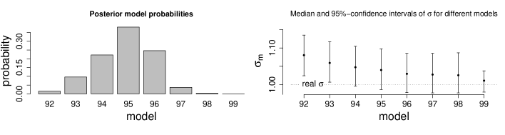
Figure 2: Posterior distribution of model number $m$ with 5%, 50%, and 95% posterior confidence intervals of the corresponding noise levels.

Note that $\sigma_{m}$ decreases with higher model order $m$ since a model comprising more sinusoids accounts for more noise. Here, we choose model $m=95$ corresponding to the posterior mode of $m$ as the best fitting model.

We used all MCMC samples corresponding to model ${\cal M}_{95}$. For ease of notation, we denote the parameter vector of model ${\cal M}_{95}$ by $(A_{1},B_{1},f_{1},\ldots,A_{95},B_{95},f_{95})$. The complete line power spectrum density can be estimated by the product of the conditional expectation of the energy $E(A_{i}^{2}+B_{i}^{2}|\mbox{\boldmath$d$},m,f_{i})$ of each sinusoid $i$ given its frequency $f_{i}$, and the posterior pdf of $f_{i}$ given the data, $p(f_{i}|\mbox{\boldmath$d$})$. One of the advantages of the Bayesian spectrum analysis is the possibility to calculate confidence areas for the spectrum. Therefore we group our MCMC samples and calculate posterior confidence intervals for each frequency bin. A sufficient width for the bins can be assessed by the frequency accuracy $\sigma_{f}=(2\pi\cdot\textrm{snr})^{-1}(48/N^{3})^{1/2}$ given by [17], where ‘snr’ is the signal-to-noise ratio. In our example, the choice of 30 000 bins is sufficient to resolve sinusoids with an snr of about $2$. Fig. 3 shows the real signals, the Bayes spectrum and the classical Schuster periodogram mentioned in Eq. 13.

Figure 3: Comparison of real signals, classical Schuster periodogram, and Bayesian spectrum. Note that the total energy of the three spectra is similar but the lines have different accuracies. Therefore the energy of a single line is more concentrated due to the better accuracy of the Bayesian spectrum estimate resulting in higher peaks. The theoretical spectrum consists of delta functions for each sinusoid which would yield infinite peaks. Therefore, an energy contribution of $\frac{N}{2}(A_{i}^{2}+B_{i}^{2})$ for each sinusoid with frequency $f_{i}$ is shown.

The plot for the real signals displays an individual energy contribution for each sinusoid $i$ of $(A_{i}^{2}+B_{i}^{2})N/2$. Normally a theoretical spectrum would consist of delta functions with infinitely large energy peaks since the energy contribution is concentrated on an interval of infinitely small width. Therefore we just plotted the energy contribution on the energy scale that yields a similar scaling as obtained by the periodogram.

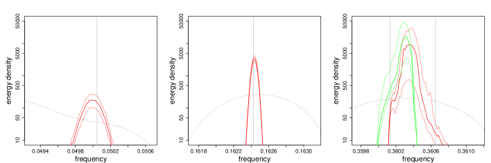
(a) Median and 95% confidence area of energy for sinusoid: E=78.2 [45.96,119.9] Energies from corresponding real parameters: E=49.9 at f=0.0500462

(b) Median and 95% confidence area of energy for sinusoid: E=476.1 [389.9,570.7] Energies from corresponding real parameters: E=459.5 at f=0.162425

(c) Median and 95% confidence area of energy for sinusoids: E=3497.2 [819.7,10800.8] E=2731.6 [261.8,8809.1] Energies from corresponding real parameters: E=462.7 at f=0.360133 E=66.9 at f=0.36065

Figure 4: Three magnified areas for a comparison of the classical periodogram (dotted line) and the 95% confidence area (area within bright colored lines) of the Bayesian spectrum. The darker colors within the 95% confidence area indicate the median of the energy. The vertical lines show the delta functions of the theoretical spectrum. Its energies are given above.

In order to be able to display 95% confidence areas of the spectrum we present three magnified areas in Fig. 4. In plot (a) we see a sinusoid with rather small energy. The accuracy of the frequency estimation is worse compared with the sinusoid of graph (b) which has a significantly larger energy. The third graph shows two very close sinusoids. The frequency estimation is very inaccurate due to the interference of the two signals. This is consistent with theoretical results by [17]. The interference of the two close signals is due to a phase shift of $175^{\circ}$. The interference and hence the frequency estimation depends upon whether the sinusoids are orthogonal [17] or not. Nevertheless, we are able to identify the existence of two signals while the periodogram only reveals the existence of one.

The estimates of the amplitudes, however, always show huge values and confidence intervals for sinusoids close in frequency. The huge energies are merely restricted by the choice of priors for the amplitudes. The reason for this is due to the possible combinations to express a sum of sinusoids when the observation time is insufficiently long with respect to the distance in frequency. In this case we can not make accurate statements about the amplitudes and hence energies of both sinusoids.

If we take a look at the single peak of the periodogram the energy that is considered is subject to the data from a discrete and finite observation time, given by $\sum_{j=1}^{N}{\mathrm{f}_{m}(t_{j},\mbox{\boldmath$a$}_{m})}$. This, however does not reflect the energy contribution of the real signals. The Bayesian estimates of the amplitudes are honest by yielding large confidence areas for the energies of sinusoids close in frequencies but in return small confidence intervals for isolated sinusoids.

5 Discussion

We have presented a Bayesian approach to identifying a large number of unknown periodic signals embedded in noisy data. A reversible jump MCMC technique can be used to estimate the number of signals present in the data, their parameters, and the noise level. This approach allows for simultaneous detection and parameter estimation, and does not require a stopping criterion for determining the number of signals. The MCMC method compares favorably with classical spectral techniques.

Our motivation for this research is to address the difficulty that LISA will ultimately encounter in having too many signals present. LISA may see 100 000 signals from binary systems in the 1 mHz to 5 mHz band. We see our work as a new method that could help LISA to identify and characterize these signals. The work here is a simplified problem, one that neglects the time evolution of the signal and modulation due to LISA’s orbit. The next step is to deal with these more complicated signals, and to develop a realistic strategy for applying our MCMC methods to more realistic LISA data. We believe that MCMC methods, like those presented here, provide a practical and highly effective method of identifying and characterizing the large number of signals that will exist in the LISA data.

References

References

- [1] K. Danzmann and A. Rüdiger, Classical and Quantum Gravity 20, S1 (2003)
- [2] L. Barak and C. Cutler, Physical Review D 70, 122002 (2004)
- [3] M.J. Benacquista, J. DeGoes, D. Lunder, Classical and Quantum Gravity 21, S509-S514 (2004)
- [4] J. Crowder and N.J. Cornish, Physical Review D 70, 082004 (2004)
- [5] G. Nelemans, L.R. Yungleson and S.F. Protegies Zwart, Astronomy and Astrophysics, 375, 890 (2001)
- [6] W.R. Gilks and S. Richardson and D.J. Spiegelhalter, Markov Chain Monte Carlo in Practice, Chapman and Hall, London (1996).
- [7] N. Metropolis, A.W. Rosenbluth, M.N. Rosenbluth, A.H. Teller, E. Teller, Journal of Chemistry and Physics 21, 1087 (1953).
- [8] W.K. Hastings, Biometrika 57, 97 (1970).
- [9] N. Christensen, R. Meyer and A. Libson, Class. Quant. Grav. 21, 317 (2004).
- [10] N. Christensen, R.J. Dupuis, G. Woan and R. Meyer, Phys. Rev D 70, 022001 (2004).
- [11] R. Umstätter, R. Meyer, R.J. Dupuis, J. Veitch, G. Woan and N. Christensen, Classical and Quantum Gravity 21, S1655 (2004).
- [12] R Umstätter, N Christensen, M Hendry, R Meyer, V Simha, J Veitch, S Vigeland and Graham Woan, Bayesian Modeling of source confusion in LISA data, pre-print.
- [13] E.T. Jaynes and G. L. Bretthorst , Probability Theory : The Logic of Science, (Cambridge University Press) (2003).
- [14] N.J. Cornish and S. L. Larson Physical Review D 67 103001 (2003)
- [15] S. Richardson and P.J. Green, J.R.Statist. Soc. B 59, 731 (1997).
- [16] C. Andrieu, A. Doucet, IEEE Trans. Sig. Proc. 47, 2667 (1999).
- [17] G. L. Bretthorst, Bayesian Spectrum Analysis and Parameter Estimation, (Springer Lecture Notes in Statistics #48), (1988).
- [18] P.J. Green, Biometrika 82, 711 (1995)
- [19] P.J. Green, In Highly Structured Stochastic Systems (Green, P.J., Hjort, N.L., Richardson, S., editors), Oxford University Press (2003)
- [20] A. Mira Ordering, Slicing and Splitting Monte Carlo Markov chain PhD thesis, University of Minnesota (1998)
- [21] L. Tierney and A. Mira Statistics in Medicine 18 2507 (1999)
- [22] P. J. Green and A. Mira, Biometrika 88, 1035 (2001)
- [23] E. T. Jaynes, Bayesian Spectrum Analysis and Chirp Analysis, Maximum Entropy and Bayesian Spectral Analysis and Estimation Problems, C. Ray Smith, and G.J. Erickson, ed., D. Reidel, Dordrecht-Holland, 1-37 (1987)
- [24] A. Schuster, Proceedings of the Royal Society of London, 77 136 (1905)
- [25] G. Celeux, M. Hurn, C. P. Robert, Journal of the American Statistical Association 95 957-970 (2000)
- [26] J.H. Ward, Journal of the American Statistical Association, 58, 236-244 (1963)