Some Uniqueness Results for Dynamical Horizons

Abstract

We first show that the intrinsic, geometrical structure of a dynamical horizon is unique. A number of physically interesting constraints are then established on the location of trapped and marginally trapped surfaces in the vicinity of any dynamical horizon. These restrictions are used to prove several uniqueness theorems for dynamical horizons. Ramifications of some of these results to numerical simulations of black hole spacetimes are discussed. Finally several expectations on the interplay between isometries and dynamical horizons are shown to be borne out.

1 Introduction

In general relativity, the surface of a black hole is often identified with a future event horizon $E$ [1, 2] — the future boundary of the past of future null infinity, $\mathscr{I}^{+}$. This strategy is physically well motivated because $E$ is the boundary of an interior spacetime region from which causal signals can never be sent to the asymptotic observers, no matter how long they are prepared to wait. The region is therefore ‘black’ in an absolute sense. Furthermore, this identification has led to a rich body of physically interesting results such as the laws of black hole mechanics in classical general relativity and the Hawking evaporation of black holes in quantum field theory in curved spacetimes. A great deal of the current intuition about black holes comes from the spacetime geometry near event horizons of Kerr spacetimes and linear perturbations thereof.

However, in fully dynamical situations where the non-linearity of general relativity can not be ignored, the strategy faces serious limitations in a number of physical contexts. These arise from two features of event horizons. First, the notion is teleological because one can locate an event horizon only after having access to the spacetime geometry to the infinite future. Second, it is ‘unreasonably’ global: it depends on a delicate interplay between $\mathscr{I}^{+}$ and the entire spacetime interior.

The first feature has direct impact, for example, on numerical simulations of black hole mergers. In these simulations one begins with initial data representing two well-separated black holes, evolves them, and studies the resulting coalescence. Since the full spacetime geometry is the end product of such a simulation, one can not use event horizons to identify black holes while setting up the initial data, nor during their evolution. In practice, the initial black holes are identified with disjoint marginally trapped surfaces (MTSs) and the aim is to study how their world tubes (called marginally trapped tubes, MTTs) evolve and merge. In the analysis of dynamics, then, one is interested in how the areas of marginally trapped surfaces grow in response to the influx of energy and angular momentum across the MTTs, how the ‘multipoles’ of the intrinsic geometry of these MTTs evolve and how they settle down to their asymptotic values. In this analysis, the event horizon plays essentially no role. Indeed, since event horizons can form in a flat region of spacetime (see, e.g., [3]) and grow in anticipation of energy that will eventually fall across them, in the fully non-linear regime changes in the geometry of the event horizon have little to do with local physical processes. Thus, because of its teleological nature, in numerical simulations the notion of an event horizon has limited use in practice.

The extremely global nature of the event horizon, on the other hand, raises issues of principle in quantum gravity. Let us go beyond quantum field theory in curved space time and examine the Hawking evaporation from the perspective of full quantum gravity. Then, it is reasonable to expect that the singularity of the classical theory is an artefact of pushing the theory beyond its domain of validity. Quantum gravity effects would intervene before the singularity is formed and the ‘true’ quantum evolution may be well-defined across what was the classical singularity. This would drastically change the global structure of spacetime. Even if the full spacetime is asymptotically flat (with a complete $\mathscr{I}^{+}$), there may well be ‘small regions around what was the classical singularity’ in which geometry is truly quantum mechanical and can not be well-approximated by any continuous metric. Since there would be no light cones in this region, the notion of the past of $\mathscr{I}^{+}$ would become ambiguous and the concept of an event horizon would cease to be useful. Problems continue to arise even if we suppose that the modifications in the neighborhood of what was a singularity are ‘tame’. Indeed, Hajicek [5] has shown that one can alter the structure of the event horizon dramatically —and even make it disappear— by changing the spacetime geometry in a Planck size neighborhood of the singularity. Thus, while the ‘true’ spacetime given to us by quantum gravity will have large semi-classical regions, there may not be a well-defined event horizon. What is it, then, that evaporates in the Hawking process? Is there an alternate way of speaking of formation and evaporation of the black hole? One would expect that if one stayed away from the neighborhood of what was a singularity, one can trust classical general relativity to an excellent degree of approximation. In these ‘classical’ regions, there are MTSs and MTTs. Since their area is known [6, 7, 9, 3] to grow during collapse and decrease because of Hawking radiation, one could use the MTTs to analyze the formation and evaporation of black holes [4].

Since they can be defined quasi-locally, the marginally trapped tubes are free of the teleological and global problems of event horizons. The above considerations suggest that, in certain contexts, they can provide a useful quasi-local description of black holes. Therefore, it is well worthwhile –and, in quantum theory, may even be essential— to understand their structure. A decade ago, Hayward [6, 7] began such an analysis and over the last four years there has been significant progress in this direction (for a review, see [3]). In broad terms, the situation can be summarized as follows. If an MTT is spacelike, it is called a dynamical horizon (DH). Under certain genericity conditions (spelled out in section 2.2) it provides a quasi-local representation of an evolving black hole. If it is null, it provides a quasi-local description of a black hole in equilibrium and is called an isolated horizon (IH). If the MTT is timelike, causal curves can transverse it in both inward and outward directions, whence it does not represent the surface of a black hole in any useful sense. Therefore it is simply called a timelike membrane (TLM). Isolated and dynamical horizons have provided extremely useful structures for numerical relativity, black hole thermodynamics, quantum gravity and mathematical physics of hairy black holes [10, 11, 8, 9, 12]. For instance, using Hamiltonian methods which first provided the notions of total mass and angular momentum at spatial infinity, it has been possible to define mass and angular momentum of DHs [13]. There exist balance laws relating values of these quantities on two MTSs of a DH and energy and angular momentum fluxes across the portion of the DH bounded by them. These notions have been useful in extracting physics from numerical simulations (see, e.g., [14, 15, 16, 3]). They have also led to integral generalizations of the differential first law of black hole mechanics, now covering processes in which the dynamics can not be approximated by a series of infinitesimal transitions from one equilibrium state to a nearby one. Thus, DHs have provided a number of concrete insights in to fully non-linear processes that govern the growth of black holes in exact general relativity.

However, as a representation of the surface of an evolving black hole, general DHs appear to have a serious drawback: a given trapped region which can be intuitively thought of as containing a single black hole may admit many dynamical horizons. While results obtained to date would hold on all of them, it is nonetheless important to investigate if there is a canonical choice or at least a controllable set of canonical choices. The lack of uniqueness could stem from two potential sources. The first is associated with the fact that a DH $H$ comes with an assigned foliation by MTSs. One is therefore led to ask: Can a given spacelike 3-manifold $H$ admit two distinct foliations by MTSs? If so, the two would provide distinct DH structures in the given spacetime. The second question is more general: Can a connected trapped region of the spacetime admit distinct spacelike 3-manifolds $H$, each of which is a dynamical horizon? Examples are known [17] in which the marginally trapped tubes have more than one spacelike portions which are separated by timelike and null portions. This type of non-uniqueness is rather tame because the DHs lie in well separated regions of spacetime. It would be much more serious if one could foliate a spacetime region by DHs. Can this happen? If there is genuine non-uniqueness, can one introduce physically reasonable conditions to canonically select ‘preferred’ DHs?

The purpose of this paper is to begin a detailed investigation of these uniqueness issues. Using a maximum principle, we will first show that if a 3-manifold $H$ admits a DH structure, that structure is unique, thereby providing a full resolution of the first set of uniqueness questions. For the second set of questions, we provide partial answers by introducing additional mild and physically motivated conditions. In particular, we will show that DHs are not so numerous as to provide a foliation of a spacetime region. Some of our results have direct implications for numerical relativity which are of interest in their own right, independently of the uniqueness issue.

The paper is organized as follows. Section 2 is devoted to preliminaries. We briefly recall the basics of the DH theory and aspects of causal theory that are needed in our analysis. We also introduce the notion of a regular DH by imposing certain mild and physically motivated restrictions. In section 3, we show that the MTS-foliation of a dynamical horizon is unique. Section 4 establishes several constraints on the location of trapped and marginally trapped surfaces in the vicinity of a regular DH. These are then used to obtain certain restrictions on the occurrence of regular DHs, which in turn imply that the number of regular DHs satisfying physically motivated conditions is much smaller than what one might have a priori expected. In section 5 we obtain certain implications of our main results which are of interest to numerical relativity. Section 6 discusses restrictions on the existence and structure of DHs in presence of spacetime Killing vectors. We conclude in section 7 with a summary and outlook.

We will use the following conventions. By spacetime $({\mathcal{M}},g)$ we will mean a smooth, connected, time-oriented, Lorentzian manifold equipped with a metric of Lorentzian signature. (By ‘smooth’ we mean ${\mathcal{M}}$ is $C^{k+1}$ and $g$ is $C^{k}$ with $k\geq 2$.) The torsion-free derivative operator compatible with $g$ is denoted by $\nabla$. The Riemann tensor is defined by $R_{abc}{}^{d}W_{d}:=2\nabla_{[a}\nabla_{b]}W_{c}$, the Ricci tensor by $R_{ab}:=R_{acb}{}^{c}$, and the scalar curvature by $R:=g^{ab}R_{ab}$. We will assume Einstein’s field equations

$$R_{ab}-\frac{1}{2}R\,g_{ab}+\Lambda g_{ab}=8\pi GT_{ab}.$$ (1.1)

For most of our results we will assume that the null energy condition (NEC) holds: for all null vectors $\ell$, the Ricci tensor satisfies $R_{ab}\ell^{a}\ell^{b}\geq 0$ or, equivalently, matter fields satisfy $T_{ab}\ell^{a}\ell^{b}\geq 0$.

We do not make an assumption on the sign or value of the cosmological constant. For definiteness, the detailed discussion will be often geared to the case when ${\mathcal{M}}$ is 4-dimensional. However, most of our results hold in arbitrary number of dimensions. Finally, the trapped and marginally trapped surfaces are only required to be compact; they need not be spherical.

2 Preliminaries

2.1 Aspects of Causal Theory

For the convenience of the reader, and in order to fix various notations and conventions, we recall here some standard notions and results from the causal theory of spacetime, tailoring the presentation to our needs. For details, we refer the reader to the excellent treatments of causal theory given in [20, 2, 21, 22]. By and large, we follow the conventions in [2, 21].

Let $({\mathcal{M}},g)$ be a spacetime. We begin by recalling the notations for futures and pasts. $I^{+}(p)$ (resp., $J^{+}(p)$), the timelike (resp., causal) future of $p\in{\mathcal{M}}$, is the set of points $q\in{\mathcal{M}}$ for which there exists a future directed timelike (resp., causal) curve from $p$ to $q$. Since small deformations of timelike curves remain timelike, the sets $I^{+}(p)$ are always open. However, the sets $J^{+}(p)$ need not in general be closed. More generally, for $A\subset{\mathcal{M}}$, $I^{+}(A)$ (resp., $J^{+}(A)$), the timelike (resp., causal) future of $A$, is the set of points $q\in{\mathcal{M}}$ for which there exists a future directed timelike (resp., causal) curve from a point $p\in A$ to $q$. Note, $I^{+}(A)=\cup_{p\in A}I^{+}(p)$, and hence the sets $I^{+}(A)$ are open. The timelike and causal pasts $I^{-}(p)$, $J^{-}(p)$, $I^{-}(A)$, $J^{-}(A)$ are defined in a time dual manner.

We recall some facts about global hyperbolicity. Strong causality is said to hold at $p\in{\mathcal{M}}$ provided there are no closed or ‘almost closed’ causal curves passing through $p$ (more precisely, provided $p$ admits arbitrarily small neighborhoods $U$ such that any future directed causal curve which starts in and leaves $U$ never returns to $U$). $({\mathcal{M}},g)$ is strongly causal provided strong causality holds at each of its points. $({\mathcal{M}},g)$ is said to be globally hyperbolic provided (i) it is strongly causal and (ii) the sets $J^{+}(p)\cap J^{-}(q)$ are compact for all $p,q\in{\mathcal{M}}$. The latter condition rules out the occurrence of naked singularities in ${\mathcal{M}}$. Globally hyperbolic spacetimes are necessarily causally simple, by which is meant that the sets $J^{\pm}(A)$ are closed whenever $A$ is compact. Thus, in a globally hyperbolic spacetime, $\partial J^{+}(A)=J^{+}(A)\setminus I^{+}(A)$ for all compact subsets $A$. This implies that, if $q\in\partial J^{+}(A)\setminus A$, with $A$ compact, there exists a future directed null geodesic from a point in $A$ to $q$. Indeed, any causal curve from a point $p\in A$ to $q\in\partial J^{+}(A)\setminus A$ must be a null geodesic (when suitably parameterized), for otherwise it could be deformed to a timelike curve from $p$ to $q$, implying $q\in I^{+}(A)$.

Even when spacetime itself is not globally hyperbolic, one can sometimes identify certain globally hyperbolic subsets of spacetime, as described further below. A subset $U\subset{\mathcal{M}}$ is said to be globally hyperbolic provided (i) strong causality holds at each point of $U$, and (ii) the sets $J^{+}(p)\cap J^{-}(q)$ are compact and contained in $U$ for all $p,q\in U$.

Global hyperbolicity can be characterized in terms of the domain of dependence. Let $S$ be a smooth spacelike hypersurface in a spacetime $({\mathcal{M}},g)$, and assume $S$ is achronal, by which is meant that no two points of $S$ can be joined by a timelike curve. (A spacelike hypersurface is always locally achronal, but in general achronality can fail in-the-large.) $S$ will not in general be a closed subset of spacetime. (In our applications, $S$ will correspond to a dynamical horizon, defined in section 2.2.) The past domain of dependence of $S$ is the set $D^{-}(S)$ consisting of all points $p\in{\mathcal{M}}$ such that every future inexendendible causal curve from $p$ meets $S$. Physically, $D^{-}(S)$ is the part of spacetime to the past of $S$ that is predictable from $S$. The past Cauchy horizon of $S$, $H^{-}(S)$, is the past boundary of $D^{-}(S)$; formally, $H^{-}(S)=\{x\in\overline{D^{-}(S)}:I^{-}(x)\cap D^{-}(S)=\emptyset\}$. Note, by its definition, $H^{-}(S)$ is a closed subset of spacetime, and is always achronal. We record the following elementary facts: (i) $S\subset D^{-}(S)$ and $D^{-}(S)\setminus S$ is open, (ii) $D^{-}(S)\cap H^{-}(S)=\emptyset$, (iii) $\overline{D^{-}(S)}=D^{-}(S)\cup H^{-}(S)$, and (iv) $\partial D^{-}(S)=S\cup H^{-}(S)$. The future domain of dependence $D^{+}(S)$ and future Cauchy horizon $H^{+}(S)$ are defined in a time-dual manner, and of course satisfy time-dual properties. The full domain of dependence $D(S)=D^{+}(S)\cup D^{-}(S)$ has the following important property: $D(S)$ is an open globally hyperbolic subset of spacetime. By definition, $S$ is a Cauchy surface for $({\mathcal{M}},g)$ provided $D(S)={\mathcal{M}}$. Hence, if $S$ is a Cauchy surface for $({\mathcal{M}},g)$, $({\mathcal{M}},g)$ is globally hyperbolic. The converse also holds, i.e., if $({\mathcal{M}},g)$ is globally hyperbolic then it admits a Cauchy surface.

2.2 Horizons

In this sub-section we will summarize the definition and basic properties of dynamical horizons that will be used in the main body of the paper. For further details see, e.g., [3].

We begin by giving the precise definitions of certain notions which were introduced in a general way in section 1. By a (future) trapped surface (TS) we will mean a smooth, closed, connected spacelike 2-dimensional submanifold of $({\mathcal{M}},g)$ both of which null normals $\ell,n$ have negative expansions. A (future) marginally trapped surface is a smooth, closed, connected spacelike 2-dimensional submanifold of $({\mathcal{M}},g)$ with the property that one of its null normals, denoted $\ell$, has zero expansion and the other, $n$, has negative expansion. While these two notions are standard, in our discussion we will often use a third, related notion. By a (future) weakly trapped surface (WTS), we will mean a smooth, closed, connected, spacelike 2-dimensional submanifold of $({\mathcal{M}},g)$ the expansions of both of whose null normals are nowhere positive. Finally, in certain situations, e.g., asymptotically flat contexts, one of the two null normals to a closed spacelike 2-manifold $S$ can be singled out as being ‘outward pointing’ and the other as being ‘inward pointing’. For such surfaces $S$, one can introduce an additional notion that will be useful occasionally. $S$ will be said to be outer marginally trapped (OMT) if the outward null normal $\ell$ has zero expansion. Note that every MTS is WTS. It is also OMT if the null normal with zero expansion is pointing outward. However, there is no simple relation between weakly trapped and outer marginally trapped surfaces. On a WTS, expansions of both null normals are restricted but one does not need to know which of them is outward pointing. The notion of an OMT surface, on the other hand, restricts the expansion only of the outward pointing normal.

A marginally trapped tube (MTT) is a smooth, 3-dimensional submanifold of $({\mathcal{M}},g)$ which admits a foliation by marginally trapped surfaces. In numerical simulations of black holes, one assumes that the initial data on a Cauchy surface admit an MTS, evolves them through Einstein’s equations and locates an MTS on each subsequent constant time slice. The union of these 1-parameter family of MTSs is an important example of an MTT. If an MTT is spacelike, it is called a dynamical horizon (DH). If it is timelike, it is called a timelike membrane (TLM). If it is null, it is called a non-expanding horizon (NEH), provided the spacetime Ricci tensor is such that $-R_{ab}\ell^{b}$ is future causal. The intrinsic ‘degenerate metric’ $q$ on an NEH is ‘time-independent’ in the sense that $\mathcal{L}_{\ell}q=0$ for any null normal $\ell$. On physical grounds [10, 11, 3], one often requires that the intrinsic connection and matter fields be also time-independent. In this case, the NEH is called an isolated horizon (IH). Under certain regularity conditions, an isolated horizon provides a quasi-local description of a black hole which has reached equilibrium, while a dynamical horizon represents an evolving black hole. There is a general expectation that under physically reasonable conditions, DHs ‘settle down’ to IHs in asymptotic future [17, 15, 16, 18]. As explained in section 1, because causal curves can transverse a timelike hypersurface in both ‘inward’ and ‘outward’ directions, one does not associate a TLM with the surface of a black hole even quasi-locally.

In this paper we will deal primarily with DHs which we will denote by $H$. A priori, it may appear that a given spacelike 3-manifold could admit distinct foliations by MTSs. However, we will show in section 3 that this can not happen. The MTSs of the unique foliation of a DH will be referred to as its leaves. More general sections will be referred to simply as cross-sections. We will generally work with DHs $H$ which satisfy two additional mild conditions. A DH $H$ will be said to be regular if i) $H$ is achronal, and ii) satisfies a ‘generiticity condition’ that $\sigma_{ab}\sigma^{ab}+T_{ab}\ell^{a}\ell^{b}$ never vanish on $H$, where $\sigma_{ab}$ is the shear of the MTSs (i.e., the trace-free part of the projection to each MTS of $\nabla_{a}\ell_{b}$). Since it is spacelike, every DH $H$ is automatically locally achronal. The first regularity condition asks that it be globally achronal. Using the spacelike character of $H$, it is easy to show that the second (i.e., genericity) condition is satisfied if and only if ${\mathcal{L}}_{n}\Theta_{(\ell)}$ never vanishes on $H$ where $\Theta_{(\ell)}$ is the expansion of $\ell$ (and $\ell$ is extended off $H$ using the geodesic equation). Furthermore, if the null energy condition (NEC) holds, one can show that ${\mathcal{L}}_{n}\Theta_{(\ell)}$ is everywhere negative. This is precisely the condition used by Hayward [6, 7] in the definition of his future, outer trapping horizon (FOTH). Thus, if the NEC holds, a DH $H$ satisfies the genericity condition if and only if it is a FOTH. This condition serves to single out black hole horizons from the DHs that arise in cosmological and other contexts [19].

While the notions introduced so far are quasi-local and meaningful even in spacetimes with spatially compact Cauchy surfaces, the notion of an event horizon is well defined only in the asymptotically flat context. Technically, it requires that the spacetime be asymptotically flat in the sense that it has a complete future null infinity, $\mathscr{I}^{+}$ (for the precise definition, see, e.g., [23]). The event horizon $E$ is then defined to be $E=\partial I^{-}(\mathscr{I}^{+})$. Event horizons of stationary, asymptotically flat spacetimes provide important examples of isolated horizons. In section 4.2 and 5, we will assume standard results [1, 2] about event horizons, such as the area theorem ($E$ has nonnegative expansion, $\theta\geq 0$), and the result that WTSs cannot meet the exterior region $I^{-}(\mathscr{I}^{+})$.

3 Uniqueness of the dynamical horizon structure

With the required notions at hand, we can now establish the uniqueness of the foliation of a DH by MTSs. This uniqueness follows easily from a geometric maximum principle closely related to the geometric maximum principle of minimal surface theory.

Let $M$ be a spacelike hypersurface in a spacetime $({\mathcal{M}},g)$, with induced metric $q$. Let $\hat{\tau}$ denote the future pointing unit normal of $M$. Given two surfaces $S_{i}$, $i=1,2$, in $M$, let ${\hat{r}}_{i}$ denote the ‘outward pointing’ unit normal of $S_{i}$ within $M$, and let $\theta_{i}$ denote the null expansion scalar of $S_{i}$ with respect to the outward null normal vector ${\ell_{i}}={\hat{r}}_{i}+{\hat{\tau}}$.

Proposition 3.1

Suppose $S_{1}$ and $S_{2}$ meet tangentially at a point $p$ (with ‘outsides’ compatibly oriented, i.e., $\ell_{1}=\ell_{2}$ at $p$), such that near $p$, $S_{2}$ is to the outside of $S_{1}$. Suppose further that the null expansion scalars satisfy, $\theta_{1}\leq 0\leq\theta_{2}$. Then $S_{1}$ and $S_{2}$ coincide near $p$ (and this common surface has zero null expansion, $\theta=0$).

Remarks: Since the sign of the null expansion scalar is invariant under the scaling of the associated null field, Proposition 3.1 does not depend on the particular normalizations chosen for the null fields $\ell_{1}$ and $\ell_{2}$. The proof of Proposition 3.1 is similar to the proof of the maximum principle for smooth null hypersurfaces obtained in [24], which may be consulted for additional details (see also [25, 26] for related results and further background).

Proof: The proof is an application of the strong maximum principle for second order quasi-linear elliptic PDEs [27, 25]. We begin by setting up the appropriate analytic framework. Let $S$ be a surface in $(M,q)$, with induced metric $\tilde{q}$, and with outward null normal field $\ell=\hat{r}+\hat{\tau}$. Let $\bar{\theta}$ denote minus the expansion scalar of $S$ with respect to $\ell$, $\bar{\theta}=-\theta$. From the definition of the null expansion scalar we have,

$$\bar{\theta}=-{\tilde{K}}-{\tilde{q}}^{ab}\nabla_{a}\hat{\tau}_{b}\,,$$ (3.2)

where $\tilde{K}:={\tilde{q}}^{ab}D_{a}\hat{r}_{b}$ is the mean curvature of $S$ in $M$. We need to express the above equation in terms of relevant differential operators.

Fix a point $p$ in $S$, and a surface $\Sigma$ through $p$ tangent to $S$ at $p$. Introduce Gaussian normal coordinates along $\Sigma$ so that in a neighborhood $U\subset M$ of $p$ we have

$$U=(-\epsilon,\epsilon)\times\Sigma\,,\quad ds^{2}=d\xi^{2}+q_{ij}(t,x)dx^{i}dx^{j}\,.$$ (3.3)

where $x=(x^{1},x^{2})$ are coordinates in $\Sigma$ (and $\partial/\partial\xi$ points to the outside of $S$ at $p$). By adjusting the size of $\Sigma$ and $U$ if necessary, $S$ can be expressed in $U$ as a graph over $\Sigma$, i.e. there is a smooth function $u(x)$ on $\Sigma$, such that $S=$ graph $u=\{(u(x),x):x\in\Sigma\}$. Let $\bar{\Theta}(u)$ denote minus the expansion scalar of $S={\rm graph}\,u$. Then from (3.2) one obtains,

$$\bar{\Theta}(u)=-\mathcal{H}(u)+b(x,u,\partial u)\,,$$ (3.4)

where $\mathcal{H}$ is the mean curvature operator (for graphs over $\Sigma$), and $b(x,u,\partial u)$ is a term involving $u$ up to first order which comes from the term involving the extrinsic curvature of $M$ in (3.2) (cf., [24] for this computation in the closely related situation in which $M$ is timelike).

$\mathcal{H}$ is a second order quasi-linear operator, which, with respect to the Gaussian coordinates (3.3), can be written as

$$\mathcal{H}(u)=-a^{ij}\frac{\partial^{2}u}{\partial x^{i}\partial x^{j}}+\mbox{ lower order terms in }u\,,$$ (3.5)

where $a^{ij}=a^{ij}(x,u,\partial u)$ is such that the matrix $[a^{ij}]$ is symmetric and positive definite. In fact, a computation shows that $a^{ij}=w\,\gamma^{ij}$, where $\gamma_{ij}$, $1\leq i,j\leq 2$, are the components of the induced metric $\tilde{q}$ on $S$ with respect to the coordinates $x_{1},x_{2}$, and $w=\left(1+q^{ij}(u(x),x)\,\frac{\partial u}{\partial x^{i}}\frac{\partial u}{\partial x^{j}}\right)^{-\frac{1}{2}}$. Combining (3.4) and (3.5), we obtain,

$$\bar{\Theta}(u)=a^{ij}\frac{\partial^{2}u}{\partial x^{i}\partial x^{j}}+\mbox{ lower order terms in }u\,,$$ (3.6)

where $a^{ij}$ is as described above. We conclude that $\bar{\Theta}$ is a second order quasi-linear elliptic operator.

Now focus on the surfaces $S_{1}$ and $S_{2}$ of the proposition. Introduce Gaussian coordinates as in (3.3), where $\Sigma$ is a surface in $M$ tangent to $S_{1}$ and $S_{2}$ at $p$. Again, adjusting the size of $\Sigma$ and $U$ if necessary, $S_{1}$ and $S_{2}$ can be expressed in $U$ as graphs over $\Sigma$, $S_{i}={\rm graph}\,u_{i}$, $u_{i}\in C^{\infty}(\Sigma)$, $i=1,2$, with the graph of $S_{1}$ lying below the graph of $S_{2}$. The assumptions of Proposition 3.1 become,

1. $u_{1}\leq u_{2}$ on $\Sigma$ and $u_{1}(p)=u_{2}(p)$, and

2. $\bar{\Theta}(u_{2})\leq 0\leq\bar{\Theta}(u_{1})$  on $\Sigma$.

By the strong maximum principle for second order quasi-linear elliptic operators [27, 25], $u_{1}=u_{2}$, and hence $S_{1}=S_{2}$ near $p$. $\Box$

The uniqueness of the foliation of a DH by MTSs is an immediate consequence of the following corollary. To fix notation, let $H=\bigcup_{R\in(R_{1},R_{2})}S_{R}$ denote a dynamical horizon foliated by MTSs $S_{R}$, $R_{1}<R<R_{2}$, where $R$ is the area radius.

Corollary 3.2

Let $S$ be a WTS in a DH $H=\bigcup_{R\in(R_{1},R_{2})}S_{R}$. Then $S$ coincides with one of the $S_{R}$’s.

Proof: The area radius $R$ achieves a maximum, $R_{0}$, say, on $S$ at some point $p\in S$. With respect to the outward direction (direction of increasing $R$) near $p$, $S$ satisfies $\theta\leq 0$, and $S_{R_{0}}$ satisfies $\theta=0$. Moreover, by the choice of $R_{0}$, $S$ is contained in the region $R\leq R_{0}$. It follows that $S$ and $S_{R_{0}}$ satisfy the hypotheses of Proposition 3.1, and thus, must agree near $p$. By similar reasoning, it follows that the set of points in $S$ (or $S_{R_{0}}$) where $S$ and $S_{R_{0}}$ agree is open, as well as closed, and hence they must agree globally, $S=S_{R_{0}}$. $\Box$

4 Constraints on the occurrence of MTSs and DHs

In this section we obtain some constraints on the occurrence of MTSs and DHs in the vicinity of a given regular DH. We begin by considering results about MTSs, from which results about DHs will follow straightforwardly.

4.1 Constraints on the occurrence of MTSs

Let $H=\bigcup_{R\in(R_{1},R_{2})}S_{R}$ denote a dynamical horizon foliated by MTSs $S_{R}$, $R_{1}<R<R_{2}$, where $R$ is the area radius. Let $H_{R>R_{0}}$ denote the part of $H$ for which $R>R_{0}$, i.e., $H_{R>R_{0}}=\bigcup_{R\in(R_{0},R_{2})}S_{R}$.

Our first and most basic result rules out the existence of weakly trapped surfaces (WTSs) in the past domain of dependence $D^{-}(H)$ of a DH $H$ in a spacetime satisfying the null energy condition.

Theorem 4.1

Let $H$ be a regular DH in a spacetime $({\mathcal{M}},g)$ satisfying the NEC. Then there are no weakly trapped surfaces (WTSs) contained in $D^{-}(H)\setminus H$.

Theorem 4.1 implies that one can not foliate a region of space-time with regular DHs even locally. However, it does not rule out the existence of a WTS $\Sigma$ not entirely contained in $D^{-}(H)\setminus H$. The next two results allow for this possibility and then restrict the location of such a WTS. In these results, it is assumed that $\Sigma$ does not meet $H^{-}(H)$, the past Cauchy horizon of $H$. Even when $\Sigma$ does not lie entirely in $D^{-}(H)$, this assumption can be met (for example, if $\Sigma$ is contained in $D^{-}(H)\cup J^{+}(H)$).

Theorem 4.2

Let $H$ be a regular DH in a spacetime $({\mathcal{M}},g)$ satisfying the NEC. Suppose $\Sigma\subset{\mathcal{M}}\setminus H^{-}(H)$ is a WTS that meets $H$ in a fixed leaf $S_{R_{0}}$. Then $\Sigma\cap D^{-}(H)$ cannot meet the causal past of $H_{R>R_{0}}$.

In fact, Theorems 4.1 and 4.2 are immediate consequences of the following more general result, which allows for a more general intersection of the WTS with $H$.

Theorem 4.3

Let $H$ be a regular DH in a spacetime $({\mathcal{M}},g)$ satisfying the NEC. Let $\Sigma$ be a WTS that does not meet $H^{-}(H)$. If $\Sigma\cap H\neq\emptyset$, set

$$R^{*}=\sup_{x\in\Sigma\cap H}R(x)\,;$$ (4.7)

otherwise set $R^{*}=R_{1}$. Then $\Sigma\cap D^{-}(H)$ cannot meet the causal past of $H_{R>R^{*}}$.

We remark that, since $H$ is closed in ${\mathcal{M}}\setminus H^{-}(H)$ and $\Sigma$ doesn’t meet $H^{-}(H)$, $\Sigma\cap H$ is compact, so that the sup in (4.7) is achieved, and hence, $R^{*}<R_{2}$ (see figure 1).

For the reader’s convenience, we will first present a rough, heuristic argument that captures the main idea of the proof. Let $\Sigma_{0}$ be the portion of $\Sigma$ in $D^{-}(H)$. Consider the intersection with $H$ of the two null hypersurfaces generated by the future directed null geodesics issuing orthogonally from $\Sigma_{0}$. One of the two, call it ${\mathcal{N}}$, will meet $H$ at a point $q$ having a largest $R$-value in this intersection. If the conclusion of the theorem does not hold then this largest $R$-value, call it $R_{0}$, will be strictly greater than $R^{*}$, $R_{0}>R^{*}$. This implies that $q$ is away from $\Sigma_{0}\cap H$, and hence is in the interior of ${\mathcal{N}}$. The NEC and the fact that $\Sigma$ is (weakly) trapped imply that ${\mathcal{N}}$ has negative expansion at $q$. By a ‘barrier argument’, this forces the expansion of the null hypersurface generated by $\ell$ along the MTS $S_{R_{0}}$ to be negative at $q$, $\Theta_{(\ell)}(q)<0$. But this contradicts the fact that $\Theta_{(\ell)}$ vanishes along $S_{R_{0}}$. While containing a number of inaccuracies, this description captures the spirit of the proof.

We now proceed to a rigorous proof. For technical reasons the barrier argument alluded to above will take place at a point slightly to the past of $H$.

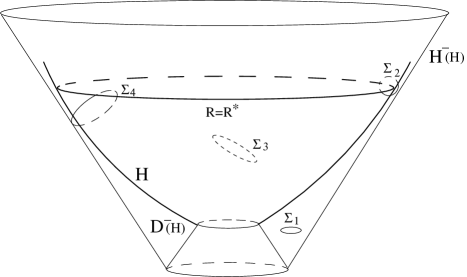
Figure 1: Examples of situations ruled out by Theorem 4.3 as well as of those that are not. Here $H$ is the dynamical horizon, $H^{-}(H)$, its past Cauchy horizon, and $D^{-}(H)$, its past domain of dependence. The compact surface $\Sigma_{1}$ lies in $D^{-}(H)\setminus H$ while $\Sigma_{3}$ lies entirely to the future of $H$. Compact surfaces $\Sigma_{2}$ and $\Sigma_{4}$ intersect $H$ and $R^{*}$ is the largest value of $R$ on their intersections with $H$. $\Sigma_{2}$ meets the causal past of $H_{R>R^{*}}$. $\Sigma_{4}$ meets $H^{-}(H)$. The theorem implies that $\Sigma_{1}$ and $\Sigma_{2}$ can not be WTSs but does not rule out the possibility that $\Sigma_{3}$ and $\Sigma_{4}$ are WTSs.

Proof of Theorem 4.3: Set $\Sigma_{0}:=\Sigma\cap D^{-}(H)$; since $\Sigma$ does not meet $H^{-}(H)$ we have, $\Sigma_{0}=\Sigma\cap(D^{-}(H)\cup H^{-}(H))=\Sigma\cap\overline{D^{-}(H)}$, and hence $\Sigma_{0}$ is compact.

The full domain of dependence of $H$, $D(H)=D^{+}(H)\cup D^{-}(H)$, is an open globally hyperbolic subset of spacetime, and $H$ is a Cauchy surface for $D(H)$, viewed as a spacetime in its own right. Thus, by restricting to $D(H)$, we may assume without loss of generality that spacetime $({\mathcal{M}},g)$ is globally hyperbolic, and $H$ is a Cauchy surface for it.

Assume, contrary to the stated conclusion, that $\Sigma_{0}$ meets the causal past of $H_{R>R^{*}}$. Then, $J^{+}(\Sigma_{0})$ meets $H_{R>R^{*}}$. Since $H$ is Cauchy and $\Sigma_{0}$ is compact, $A:=J^{+}(\Sigma_{0})\cap H$ is a compact subset of $H$. Let $R_{0}=\sup_{x\in A}R(x)$. Since $A$ is compact this sup is achieved for some point $q\in A$ and hence $R(q)=R_{0}$. Clearly, $q$ must lie on the boundary of $A$ in $H$, which implies that $q\in\partial J^{+}(\Sigma_{0})=J^{+}(\Sigma_{0})\setminus I^{+}(\Sigma_{0})$. Since $J^{+}(\Sigma_{0})$ meets $H_{R>R^{*}}$, it follows that $R_{0}>R^{*}$, and hence $q$ is not on $\Sigma_{0}$. Thus, there exists a future directed null geodesic segment $\eta$ extending from a point $p\in\Sigma_{0}\setminus H$ to $q$. Note that $\eta$ must meet $\Sigma_{0}$ orthogonally at $p$, for otherwise, by a small deformation of $\eta$, there would exist a timelike segment from a point on $\Sigma_{0}$ to a point on $\eta$, which would imply that $q$ is in $I^{+}(\Sigma_{0})$. For similar reasons, there can be no null geodesic, distinct from $\eta$, joining a point of $\Sigma_{0}$ to a point of $\eta$ prior to $q$, and there can be no null focal points to $\Sigma_{0}$ along $\eta$ prior to $q$ [21]. Then, by standard [21, 22] results, we know that the congruence of future directed null geodesics near $\eta$, issuing orthogonally to $\Sigma_{0}$ from points on $\Sigma_{0}$ near $p$, forms a smooth null hypersurface in a neighborhood of $\eta\setminus\{q\}$. (We need to avoid $q$, due to the possibility that it may be a focal point, and hence a point where smoothness may break down.) Call this null hypersurface ${\bf N_{1}}$ (see figure 2).

Now consider the smooth null hypersuface ${\bf N_{2}}$, defined in a neighborhood of $S_{R_{0}}$, generated by the null geodesics passing through the points of $S_{R_{0}}$ in the direction of the outward null normal $\ell$ along $S_{R_{0}}$. We wish to compare ${\bf N_{1}}$ and ${\bf N_{2}}$ near $q$. To make this comparison, we first observe that $\eta$ meets $S_{R_{0}}$ orthogonally at $q$. For if it didn’t, there would exist a timelike curve from a point of $\eta$ to a point $y\in S_{R_{0}}$. Hence, $y\in I^{+}(\Sigma_{0})$ would be an interior point of $A$ satisfying $R(y)=R_{0}$. But this would mean that there are points $x$ in $A$ with $R(x)>R_{0}$, contradicting the choice of $q$. Thus, $\eta$ meets $S_{R_{0}}$ orthogonally, and hence, $\eta^{\prime}|_{q}$, the tangent vector to $\eta$ at $q$, points in the direction either of the outward null normal $\ell|_{q}$ or the inward null normal $n|_{q}$. But note, in the latter case, there would exist a timelike curve from a point on $\eta$ slightly to the past of $q$ to a point $z\in H$ satisfying, $R(z)>R_{0}$, again contradicting the choice of $q$.

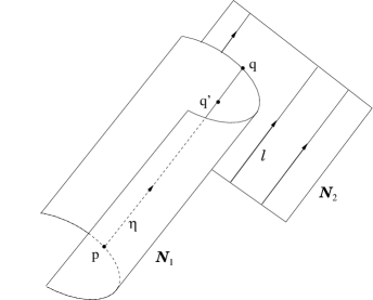
Figure 2: Null hypersurfaces ${\bf N_{1}}$ and ${\bf N_{2}}$. ${\bf N_{1}}$ is generated by future directed null geodesics issuing orthogonally to $\Sigma_{0}$ from points near $p$ in $\Sigma_{0}$. ${\bf N_{2}}$ is generated by null geodesics along $\ell$, passing through points of $S_{R_{0}}$ near $q$. The segment near $q^{\prime}$ of the null geodesic $\eta$ lies on both null surfaces.

We conclude from the preceding paragraph that, at $q$, the tangent vector $\eta^{\prime}$ points in the same direction as $\ell|_{q}$; by choosing the affine parameter of $\eta$ suitably, we may assume $\eta^{\prime}|_{q}=\ell|_{q}$. It follows that, near, but prior to $q$, $\eta$ is a common null generator of ${\bf N_{1}}$ and ${\bf N_{2}}$, and ${\bf N_{1}}$ and ${\bf N_{2}}$ are tangent along $\eta$. Choose a point $q^{\prime}$ on $\eta$ slightly to the past of $q$; we will be a bit more specific about the choice of $q^{\prime}$ in a moment. For $i=1,2$, let $\theta_{i}$ denote the expansion of the null generators of ${\bf N_{i}}$, as determined by the tangent null vector field $\ell_{i}$; $\ell_{1}$ and $\ell_{2}$ may be scaled so as to agree along $\eta$. We want to compare $\theta_{1}$ and $\theta_{2}$ at $q^{\prime}$. We know that ${\bf N_{1}}$ and ${\bf N_{2}}$ are tangent at $q^{\prime}$. Furthermore, in a suitably chosen small neighborhood of $q^{\prime}$, ${\bf N_{1}}$ must lie to the future side of ${\bf N_{2}}$. Indeed, if this were not the case, there would exist a point $w^{\prime}$ on ${\bf N_{2}}$ which is in the timelike future of a point on ${\bf N_{1}}$. Following the generator of ${\bf N_{2}}$ through $w^{\prime}$ to the future, we obtain a point $w\in S_{R_{0}}$ which is in the interior of $A$, again contradicting the choice of $q$.

From the fact that ${\bf N_{1}}$ and ${\bf N_{2}}$ are tangent at $q^{\prime}$, and that near $q^{\prime}$, ${\bf N_{1}}$ lies to the future side of ${\bf N_{2}}$, it follows that the generators of ${\bf N_{1}}$ diverge at least as much as the generators of ${\bf N_{2}}$ at $q^{\prime}$, i.e., one must have the inequality,

$$\theta_{1}(q^{\prime})\geq\theta_{2}(q^{\prime})\,.$$ (4.8)

Since $\Sigma$ is a WTS, we know that $\theta_{1}(p)\leq 0$. Moreover, Raychaudhuri’s equation for a null geodesic congruence, in conjunction with the null energy condition, implies that ${\mathcal{L}}_{\ell_{1}}(\theta_{1})\leq 0$ along $\eta$, i.e. $\theta_{1}$ is nonincreasing to the future along $\eta$. This implies that $\theta_{1}(q^{\prime})\leq 0$, and hence by (4.8) that $\theta_{2}(q^{\prime})\leq 0$. On the other hand, since $S_{R_{0}}$ is an MTS, $\theta_{2}(q)=\Theta_{(\ell)}|_{q}=0$. Further, since $n-\ell$ is tangent to $H$, we have ${\mathcal{L}}_{n-\ell}(\Theta_{(\ell)})\equiv 0$. Hence, ${\mathcal{L}}_{-\ell_{2}}(\theta_{2})|_{q}={\mathcal{L}}_{-\ell}(\Theta_{(\ell)})|_{q}=-{\mathcal{L}}_{n}(\Theta_{(\ell)})|_{q}+{\mathcal{L}}_{n-\ell}(\Theta_{(\ell)})|_{q}=-{\mathcal{L}}_{n}(\Theta_{(\ell)})|_{q}$. Thus, the genericity condition implies that ${\mathcal{L}}_{-\ell_{2}}(\theta_{2})|_{q}>0$. It follows that if $q^{\prime}$ is taken sufficiently close to $q$, $\theta_{2}(q^{\prime})$ will be strictly positive, and we arrive at a contradiction.  $\Box$

By arguments similar to those used to prove Theorem 4.1, one may obtain the time-dual conclusion of that theorem that there are no past weakly trapped surfaces contained in $D^{+}(H)\setminus H$. This result is of physical interest in spherically symmetric space-times because it implies that every round sphere in $D^{+}(H)\setminus H$ is (future) trapped. However, we are now considering general space-times and our present task is to restrict the location of (future) MTSs in the vicinity of $H$, for which the exact time-dual can not be directly used.

Nevertheless, there is a partial time dual that does apply. To formulate it, we need first to introduce a couple of definitions. By a cross-section of a DH $H$ we mean a compact surface $S\subset H$ that is a graph, $R=R(x)$, over some fixed MTS $S_{R_{0}}$. Then it makes sense to talk about points or sets in $H$ that lie above or below $S$; e.g., $A\subset H$ lies below $S$ provided $A$ is contained in the region $\{R\leq R(x)\}$, etc.. We will say that a MTS $\Sigma$ in $D^{+}(H)\setminus H$ can be properly joined to $H$ if there exist a cross-section $S$ of $H$ and a spacelike, compact hypersurface $M\subset D^{+}(H)$ with boundary $\Sigma\cup S$ such that: i) $M\cap H=S$, ii) $J^{-}(M)\cap H$ lies below $S$, and iii) the projection onto $M$ of the null normal $\ell$ to $\Sigma$ with zero expansion points towards $S$ everywhere on $\Sigma$ (see figure 3).

The following result is then the desired partial time dual of Theorem 4.1.

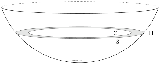
Figure 3: $H$ is a dynamical horizon. Theorem 4.4 implies that a 2-surface like $\Sigma$ can not be marginally trapped.

Theorem 4.4

Let $H$ be a regular DH in a spacetime $({\mathcal{M}},g)$ satisfying the NEC. Then there does not exist an MTS $\Sigma$ in $D^{+}(H)\setminus H$ that can be properly joined to $H$.

Comments on the proof: The proof is essentially the time dual of the proof of Theorem 4.3. Assuming the existence of such an MTS $\Sigma$, we set $A=J^{-}(M)\cap H$, and let $R_{0}=\inf_{x\in A}R(x)$. We choose $q\in H$ to be a point that realizes this infimum. It follows that $q\in\partial J^{-}(M)\setminus M$, and since $\partial J^{-}(M)=J^{-}(M)\setminus I^{-}(M)$, we obtain a past directed null geodesic $\eta$ from a point $p\in M$ to $q$. By arguments similar to those used before, in order to avoid $q\in I^{-}(M)$ it must be that (1) $p\in\Sigma$, (2) $\eta$ meets $\Sigma$ orthogonally at $p$, and (3) $\eta^{\prime}$ points in the direction of $-\ell$ (rather than $-n$) at $p$. The main role of the ‘properly joined to $H$’ condition is to insure that this third condition holds. Since $-\ell$ has nonpositive (in fact zero) expansion along $\Sigma$, the proof may now proceed in precisely the same (but time-dual) manner as the proof of Theorem 4.3: We introduce the null hypersurfaces ${\bf N_{1}}$ and ${\bf N_{2}}$, the former generated by the congruence of past directed orthogonal null geodesics near $\eta$, and the latter generated by $\ell$ along $S_{R_{0}}$, and obtain a contradiction by examining the expansions of these null hypersurfaces at a point $q^{\prime}$ on $\eta$ slightly to the future of $q$. In the present situation, ${\bf N_{1}}$ lies to the past of ${\bf N_{2}}$ near $q^{\prime}$ (at which they are tangent). $\Box$

Remark: We note, as follows from the proof, that Theorem 4.4 remains valid without any condition on the expansion of the other null normal $n$ of the MTS $\Sigma$.

4.2 Constraints on the occurrence of DHs

Theorem 4.1 leads immediately to statements about the existence and location of dynamical horizons.

Corollary 4.5

Let $H$ be a regular DH in a spacetime $({\mathcal{M}},g)$ satisfying the NEC. If $H^{\prime}$ is another DH contained in $D(H)$, $H^{\prime}$ cannot lie strictly to the past of $H$. If $H^{\prime}$ ‘weaves’ $H$ (so that part of it lies to the future and part of it lies to the past of $H$), $H^{\prime}$ cannot contain an MTS which lies strictly to the past of $H$.

Proof: If either conclusion failed there would exist a WTS in $D^{-}(H)\setminus H$, contradicting Theorem 4.1. $\Box$

We note that this corollary remains valid if $H^{\prime}$ is merely a MTT.

There is a general expectation that under ‘favorable’ circumstances a marginally trapped tube that forms during a gravitational collapse becomes spacelike —i.e., a DH— soon after collapse, and asymptotically approaches the event horizon. This is based on some explicit examples such as the Vaidya spacetimes [9, 3], general analytical arguments [17], numerical simulations of the collapse of a spherical scalar field [18, 17], and of axi-symmetric collapse of rotating neutron stars [15, 16]. From a physical and astrophysical viewpoint, it is these dynamical horizons which asymptote to the event (or, more generally, isolated) horizons in the distant future that are most interesting. We now consider this situation.

Thus, for the following, we assume spacetime $({\mathcal{M}},g)$ is asymptotically flat, i.e. admits a complete $\mathscr{I}^{+}$ [23], and has an event horizon $E$, for which standard results [1, 2] are assumed to hold, cf., section 2.2. We have in mind here, and the next section, dynamical black hole spacetimes. (Results concerning stationary black holes will be considered in Section 6.) In view of this, and to avoid certain degenerate situations, we will assume that each cross section of the event horizon has at least one point at which $\theta>0$. We say that a DH $H$ is asymptotic to the event horizon $E$ if there exists an achronal spacelike hypersurface $V$ meeting $H$ in some MTS $S$ such that, in the portion of spacetime to the future of $V$, the Cauchy horizon of $H$ coincides with $E$, $H^{-}(H)\cap I^{+}(V)=E\cap I^{+}(V)$. We refer to $I^{+}(V)$ as the asymptotic region.

In this setting, Corollary 4.5 may be formulated as follows.

Corollary 4.6

Let $({\mathcal{M}},g)$ be a spacetime obeying the NEC and admitting an event horizon $E$. Let $H$ be a regular DH asymptotic to $E$. If $H^{\prime}$ is another DH contained in the asymptotic region, $H^{\prime}$ cannot lie strictly to the past of $H$. If $H^{\prime}$ ‘weaves’ $H$ (so that part of it lies to the future and part of it lies to the past of $H$), $H^{\prime}$ cannot contain an MTS which lies strictly to the past of $H$.

Proof: Let $\Sigma$ be an MTS of $H^{\prime}$ contained in $I^{-}(H)\cap I^{+}(V)$. In view of Corollary 4.5, it is sufficient to show that $\Sigma\subset D^{-}(H)$. We show first that $\Sigma\subset D^{-}(H)\cup H^{-}(H)$. Let $p$ be a point on $\Sigma$, and suppose $p\notin D^{-}(H)\cup H^{-}(H)$. Since $p\in I^{-}(H)$, there exists a future directed timelike curve $\gamma$ from $p$ to $H$. In order to reach $H$, $\gamma$ must cross $H^{-}(H)$ at a point $q$, say. Since $\Sigma$ is in the asymptotic region, we must have $q\in E=\partial I^{-}(\mathscr{I}^{+})$. Hence $p\in I^{-}(E)\subset I^{-}(\mathscr{I}^{+})$. But as a WTS, $\Sigma$ cannot meet the exterior region $I^{-}(\mathscr{I}^{+})$. Thus, $\Sigma\subset D^{-}(H)\cup H^{-}(H)$.

Suppose $\Sigma\subset I^{+}(V)$ touches $H^{-}(H)\cap I^{+}(V)=E\cap I^{+}(V)$. Then, $\Sigma$ lies inside the event horizon $E$, and touches it at some point. $\Sigma$ has expansion $\theta\leq 0$ with respect to its future null normals, and $\Sigma_{E}$, the cross section of the event horizon obtained as the intersection of $E$ with $H^{\prime}$, has expansion $\theta\geq 0$ with respect to its future, outward null normal. The maximum principle Proposition 3.1 then implies that $\Sigma$ and $\Sigma_{E}$ coincide. This forces the cross section $\Sigma_{E}$ to have vanishing expansion, contrary to assumption. It follows that $\Sigma\subset D^{-}(H)$, as was to be shown. $\Box$

5 DHs and Numerical Relativity

This section is intended to be of more direct relevance to numerical relativity. We will begin by formalizing the strategy used in black hole simulations to locate MTTs at each time step of the evolution.

Given a DH $H$, let $\{M_{t}:t_{1}<t<t_{2}\}$ be a foliation by (connected) spacelike hypersurfaces of an open set $U\subset{\mathcal{M}}$ containing $H$, given by a time function ${\mathcal{T}}$ on $U$ (i.e. $M_{t}=\{{\mathcal{T}}\!=t\}$). Suppose that each $M_{t}$ meets $H$ transversely in a unique MTS $S_{R}$ such that the area radius $R=R(t)$ is an increasing (rather than decreasing) function of $t$. Suppose further that $S_{R}$ separates $M_{t}$ into an ‘inside’ (the side into which the projection of $n$ points) and an ‘outside’ (the side into which the projection of $\ell$ points). By these conditions, the outside of $S_{R}$ in $M_{t}$ lies locally to the past of $H$, and the inside lies locally to the future of $H$. Under this set of circumstances we say that $H$ is generated by the spacelike foliation $\{M_{t}\}$.

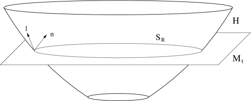
Figure 4: Illustration of a dynamical horizon $H$ which is generated by a foliation $M_{t}$. The figure shows one leaf of the foliation which intersects $H$ in a MTS $S_{R}$ of area radius $R$. $\ell$ is the outward pointing null normal to the MTSs and $n$ the inward pointing one.

The following result establishes conditions under which the MTSs of a DH are ‘outermost’.

Theorem 5.1

Let $H$ be a regular DH in a spacetime $({\mathcal{M}},g)$ satisfying the NEC. Suppose $H$ is generated by a spacelike foliation $\{M_{t}\}$ in ${\mathcal{M}}\setminus H^{-}(H)$. Let $S=S_{R_{0}}$ be the MTS of $H$ determined by the slice $M=M_{t_{0}}$. Then $S$ is the outermost WTS in $M$. That is, if $\Sigma$ is any other WTS in $M$, $\Sigma$ does not meet the region of $M$ outside of $S$.

An example in [17] shows that the MTSs of a DH $H$ can fail to be outermost in the sense of Theorem 5.1, if the spacelike foliation $\{M_{t}\}$ is allowed to meet $H^{-}(H)$.

Proof: $M$ decomposes into the disjoint union, $M={\mathcal{I}}\cup S\cup{\mathcal{O}}$, where ${\mathcal{I}}$ is the inside of $S$ and ${\mathcal{O}}$ is the outside. We want to show $\Sigma\subset{\mathcal{I}}\cup S$. Suppose, to the contrary $\Sigma$ meets ${\mathcal{O}}$. Near $S$, ${\mathcal{O}}$ is to the past of $H$, and hence meets $D^{-}(H)$. It follows that ${\mathcal{O}}\subset D^{-}(H)$. Indeed, if ${\mathcal{O}}$ were to leave $D^{-}(H)$ it would have to intersect $\partial D^{-}(H)=H\cup H^{-}(H)$. Since ${\mathcal{O}}$ does not meet $H$, it must intersect $H^{-}(H)$. But we have assumed the entire foliation misses $H^{-}(H)$.

Thus, ${\mathcal{O}}\subset D^{-}(H)$. By Theorem 4.1, $\Sigma$ cannot be entirely contained in ${\mathcal{O}}$. It follows that $\Sigma$ meets $H$ in the fixed leaf $S=S_{R_{0}}$. By Theorem 4.2, $\Sigma\cap D^{-}(H)$ cannot meet the causal past of $H_{R>R_{0}}$. Choose a point $p\in\Sigma\cap{\mathcal{O}}$. Since $p\in D^{-}(H)\setminus H$, there exists a future directed timelike curve $\gamma$ from $p$ to a point $q\in H$. By choosing $p$ sufficiently close to $S$, we can ensure that $\gamma$ is entirely contained in the foliated region. Then, since $t$, the label for the foliation $\{M_{t}\}$, increases along $\gamma$, and $R$ is an increasing function of $t$, it follows that $R>R_{0}$ at $q$, a contradiction. $\Box$

Theorem 5.1 implies, in particular, that DHs determined by a spacelike foliation $\{M_{t}\}$ can not ‘bifurcate’, i.e., there can not be two distinct DHs determined by the same spacelike foliation coming out of a common MTS. More precisely, we have the following.

Corollary 5.2

Let $H_{1}$ and $H_{2}$ be DHs generated by a spacelike foliation $\{M_{t}:t_{1}<t<t_{2}\}$ in a spacetime $({\mathcal{M}},g)$ satisfying the NEC. If, for some $t_{0}\in(t_{1},t_{2})$, the MTS of $H_{1}$ and of $H_{2}$, respectively, determined by the time slice $M_{t_{0}}$ agree, then $H_{1}=H_{2}$.

Proof: For the purposes of this proof, let $S_{1}(t)$ and $S_{2}(t)$ denote the MTSs of $H_{1}$ and $H_{2}$, respectively, in the time slice $M_{t}$. We are assuming that $S_{1}(t_{0})=S_{2}(t_{0})$, and we want to show that $S_{1}(t)=S_{2}(t)$ for all $t\in(t_{1},t_{2})$. Shrink the foliation $\{M_{t}\}$ to a neighbohood $U\subset D(H_{1})$ of $H_{1}$. Since $S_{2}(t_{0})=S_{1}(t_{0})$, there exists $\epsilon>0$ such that $S_{2}(t)\subset U$ for all $t\in(t_{0}-\epsilon,t_{0}+\epsilon)$. Then, Theorem 5.1 applied to $H_{1}$ implies that $S_{2}(t)\subset{\mathcal{I}}_{1}(t)\cup S_{1}(t)$ where ${\mathcal{I}}_{1}(t)$ is the inside of $S_{1}(t)$ in $M_{t}$, for all $t\in(t_{0}-\epsilon,t_{0}+\epsilon)$. It follows that $H_{2}$ lies to the future side of $H_{1}$ near $S_{1}(t_{0})$. This in turn implies that $H_{1}$ lies to the past side of $H_{2}$ near $S_{2}(t_{0})$. As a consequence we have that $S_{1}(t)\subset{\mathcal{O}}_{2}(t)\cup S_{2}(t)$, where ${\mathcal{O}}_{2}(t)$ is the outside of $S_{2}(t)$ in $M_{t}$, for all $t\in(t_{0}-\epsilon,t_{0}+\epsilon)$. But, by Theorem 5.1, now applied to $H_{2}$, $S_{2}(t)$ is outermost in $M_{t}$. We conclude that $S_{1}(t)=S_{2}(t)$ for all $t\in(t_{0}-\epsilon,t_{0}+\epsilon)$.

Let $A=\{t\in(t_{1},t_{2}):S_{1}(t)=S_{2}(t)\}$. The argument above shows that $A$ is open in $(t_{1},t_{2})$. Since it is also clearly closed and nonempty, we have $A=(t_{1},t_{2})$. Hence $H_{1}=H_{2}$. $\Box$

Remark: In the setting and notation of Theorem 5.1, it is possible to show that the MTS $S$ is also outermost among outer marginally trapped (OMT) surfaces in $M$ homologous to $S$. For example, by arguments similar, but time-dual, to those used to prove Theorem 4.4 (cf., also the remark after the proof), one may show that there can be no OMT surface in $M$ lying outside of $S$ that, together with $S$, bounds a region in $M$. (Such a surface would be properly joined to $S$ in a sense similar to that used in Theorem 4.4.)

In numerical simulations one is interested in foliations $M_{t}$ which start out at spatial infinity, pass through the Cauchy horizon $H^{-}(H)$ and meet $H$ in MTSs $S$. The resulting DHs $H$ are found to be asymptotic to the event horizon in the distant future. The next result is tailored to this scenario. Let $({\mathcal{M}},g)$ be a dynamical black hole spacetime, as described in section 4.2. Recall, as defined there, a DH $H$ is said to be asymptotic to the event horizon $E$ provided in the asymptotic region (i.e., the region to the future of some achronal spacelike hypersurface), the past Cauchy horizon $H^{-}(H)$ of $H$ coincides with $E$.

Theorem 5.3

Suppose $H$ is a regular DH asymptotic to the event horizon $E$ in a spacetime $({\mathcal{M}},g)$ obeying the NEC. Suppose, in the asymptotic region, $H$ is generated by a spacelike foliation $\{M_{t}\}$, such that each time slice $M_{t}$ meets E in a single (connected) cross section. Let $S=S_{R_{0}}$ be the MTS of $H$ determined by the slice $M=M_{t_{0}}$. Then $S$ is the outermost WTS in $M$. That is, if $\Sigma$ is any other WTS in $M$, $\Sigma$ does not meet the region of $M$ outside of $S$.

Proof: By restricting to the asymptotic region, we may assume that $H^{-}(H)=E$. Let $\Sigma$ be a MTS in $M$. Since $M$ meets $E$ in a single cross section $S_{E}=M\cap E$, the portion of $M$ outside of $S_{E}$ is contained in the exterior region $I^{-}(\mathscr{I}^{+})$. Since a WTS can not meet the exterior region, $\Sigma$ must be contained in the black region $B={\mathcal{M}}\setminus I^{-}(\mathscr{I}^{+})$. If $\Sigma$ touches $S_{E}$, which by the area theorem has nonnegative expansion with respect to the outward null normal, then the maximum principle Proposition 3.1 implies that $\Sigma=S_{E}$. But this forces $S_{E}$ to have vanishing expansion, contrary to the assumption we had made about dynamical black holes (cf. section 4.2). Thus, $\Sigma$ is actually contained in the interior of the black hole region, $\Sigma\subset{\rm int}\,B$. Applying Theorem 5.1 to the restricted foliation $\{M^{\prime}_{t}=M_{t}\cap{\rm int}\,B\}$, each leaf of which does not meet $H^{-}(H)=E$, we conclude that $\Sigma$ does not meet the region of $M$ outside of $S$, as was to be shown. $\Box$

In spacetimes with multiple black holes, the time slices $M_{t}$ may meet the event horizon in several cross sections. Theorem 5.3 could still be applied to this multi-black hole situation, by suitably restricting each of the time slices $M_{t}$ to a subregion meeting the event horizon in a single cross section.

Theorem 5.3, together with several previous results, leads to the following uniqueness result for dynamical horizons.

Theorem 5.4

Suppose $H_{1}$ and $H_{2}$ are regular DHs asymptotic to the event horizon $E$ in a black hole spacetime $({\mathcal{M}},g)$ obeying the NEC. Suppose, in the asymptotic region, $H_{1}$ and $H_{2}$ are generated by the same spacelike foliation $\{M_{t}\}$, where each time slice $M_{t}$ meets E in a single (connected) cross section. Then, in the asymptotic region, $H_{1}=H_{2}$.

Proof:  Without loss of generality we may restrict spacetime $({\mathcal{M}},g)$ to the asymptotic region. We first show that $H_{1}$ and $H_{2}$ meet. Since $H_{1}$ and $H_{2}$ have a common past Cauchy horizon (namely E), it follows that either $H_{2}$ meets $D^{-}(H_{1})$ or $H_{1}$ meets $D^{-}(H_{2})$. Assume the latter holds. By Corollary 4.5, $H_{1}$ can not be contained in $D^{-}(H_{2})\setminus H_{2}$. Hence, $H_{1}$ must meet $\partial D^{-}(H_{2})=H_{2}\cup H^{-}(H_{2})$. But $H^{-}(H_{2})=H^{-}(H_{1})$, and $H_{1}$ can not meet its own past Cauchy horizon. It follows that $H_{1}$ meets $H_{2}$.

Suppose $H_{1}$ and $H_{2}$ meet at $p\in M_{t_{0}}$. Let $S_{1}$ and $S_{2}$ denote the MTSs of $H_{1}$ and $H_{2}$, respectively, in the time slice $M_{t_{0}}$. Note that $p$ is on both $S_{1}$ and $S_{2}$. Theorem 5.3 applied to $H_{1}$ implies that $S_{2}$ is in the region of $M_{t_{0}}$ inside of $S_{1}$, yet meets $S_{1}$ at $p$. (Since $S_{2}$ is in the same component of $M_{t_{0}}\cap B$ ($B={\mathcal{M}}\setminus I^{-}(\mathscr{I}^{+})$) as $S_{1}$, the added condition on the time slices $M_{t}$ in Theorem 5.3 is not needed here; see the remark after the proof of Theorem 5.3.) The maximum principle Proposition 3.1 then implies that $S_{2}=S_{1}$. Now, by Corollary 5.2, $H_{1}=H_{2}$. $\Box$

In fact, Theorem 5.4 and its proof do not involve the event horizon $E$ in an essential way. It is sufficient to require that $H_{1}$ and $H_{2}$ be asymptotic to each other, by which is meant that in the asymptotic region (the region to the future of some achronal spacelike hypersurface) the past Cauchy horizons of $H_{1}$ and $H_{2}$ agree. In this more general situation, one may apply Theorem 5.1 in lieu of Theorem 5.3.

Recently, numerical simulations were performed specifically to explore the properties of MTTs [16] generated by a space-like foliation. In the case of the gravitational collapse leading to a single black hole, one begins with the foliation $M_{t}$ in the asymptotic region and searches for MTSs on each leaf. In some cases, each $M_{t}$ admits two well separated MTSs. Thus, the MTTs obtained by evolution have two branches. The outer MTT is a DH which is asymptotic to an isolated horizon while the inner one is a timelike membrane (TLM). Theorem 5.3 ensures that on any one time slice $M_{t}$, there is no MTS outside the intersection $S_{R(t)}$ of $M_{t}$ and $H$. Our next result concerns the TLM where the situation turns out to be just the opposite.

Let us first describe in somewhat more detail the setting for this result. Consider a TLM   $T$ whose MTSs $S_{t}$ are determined by a spacelike foliation $\{M_{t}\}$, i.e., $S_{t}=M_{t}\cap T$, such that $S_{t}$ separates $M_{t}$ into an ‘inside’ (the side into which the projection of $n$ points) and an ‘outside’ (the side into which the projection of $\ell$ points). We will assume that the time slices $M_{t}$ obey a very mild asymptotic flatness condition: there exists outside each $S_{t}$ in $M_{t}$ a closed surface $\tilde{S}_{t}$, such that it and $S_{t}$ form the boundary of a compact $3$-manifold $V_{t}\subset M_{t}$, and such that $\tilde{S}_{t}$ has positive expansion with respect to its outward null normal, $\tilde{\theta}_{t}>0$. Finally, we will assume that $T$ satisfies the genericity condition that the quantity $\sigma_{ab}\sigma^{ab}+T_{ab}\ell^{a}\ell^{b}$ never vanish on $T$, cf., section 2.2. Raychaudhuri’s equation, together with the NEC, then implies that ${\mathcal{L}}_{\ell}\Theta_{(\ell)}<0$ along each MTS $S_{t}$.

Proposition 5.5

Let $T$ be a TLM in a spacetime $({\mathcal{M}},g)$ satisfying the dominant energy condition. Let $T$ be determined by a spacelike foliation $\{M_{t}\}$, such that the time slices $M_{t}$ obey the mild asymptotic flatness condition described above. Assume further that $T$ obeys the genericity condition. Then there exists an OMT surface outside of each MTS $S_{t}$ in $M_{t}$.

Proof: The proposition follows from a recent result of Schoen [32]. Very briefly, consider an MTS $S_{t^{\prime}}$ slightly to the past of the MTS $S_{t}$. For $t^{\prime}$ sufficiently close to $t$, the null hypersurface generated by $\ell$ along $S_{t^{\prime}}$, will meet $V_{t}$ in a smooth closed surface $\hat{S}_{t}$ just outside $S_{t}$, such that it and $\tilde{S}_{t}$ form the boundary of a compact $3$-manifold $B_{t}\subset V_{t}$. Moreover, taking $t^{\prime}$ closer to $t$ if necessary, the genericity condition will imply that $\hat{S}_{t}$ has negative expansion, $\hat{\theta}_{t}<0$. Together with the fact that $\tilde{S}_{t}$ has positive expansion $\tilde{\theta}_{t}>0$, Schoen’s result (which requires the dominant energy condition) implies the existence of an OMT surface in the interior of $B_{t}$ (homologous, in fact, to $S_{t}$). $\Box$

Theorem 5.5 says that the existence of the TLM $T$ by itself implies that each $M_{t}$ must admit another OMT which lies outside $M_{t}\cap T$. There is no a priori guarantee that the world tube of these new OMTs would be a DH. But Theorem 5.1 suggests that the outermost MTT would be a DH. Together, Proposition 5.5 and Theorem 5.1 imply that the findings of numerical simulations [16] mentioned above are not accidental but rooted in a general structure.

6 Dynamical horizons and Killing vectors

We will now discuss some restrictions on the type of dynamical horizons that can exist in spacetimes admitting isometries. We will limit ourselves only to a few illustrative results that show that some of the intuitive expectations on the interplay between Killing symmetries and dynamical horizons are immediate consequences of the main results of sections 3 and 4.

First, since DHs are associated with evolving black holes, one would expect that stationary spacetimes do not admit DHs. This conjecture is supported by a result which holds in the more general setting of spacetimes admitting isolated horizons $\Delta$. We will say that a DH $H$ is asymptotic to an isolated horizon $\Delta$ if there exists an achronal spacelike hypersurface $V$ meeting $H$ in some MTS $S$ such that, in the portion of spacetime to the future of $V$, the Cauchy horizon of $H$ coincides with $\Delta$, i.e., $H^{-}(H)\cap I^{+}(V)=\Delta\cap I^{+}(V)$. We then have:

Theorem 6.1

Let $({\mathcal{M}},g)$ be a spacetime obeying the NEC which contains a non-expanding horizon $\Delta$. Suppose $\Delta$ admits a cross-section $S$ such that the expansion of the inward pointing null normal $n$ is negative and the expansion of the outward pointing null normal $\ell$ satisfies $\mathcal{L}_{n}\theta<0$. Then ${\mathcal{M}}$ does not admit any regular DH $H$ asymptotic to $\Delta$.

Proof: : Suppose ${\mathcal{M}}$ does admit such a DH $H$. Then, by displacing $S$ infinitesimally along $n$ we would obtain a WTS in $D^{-}(H)\setminus H$ contradicting the result of Theorem 4.1. $\Box$

Event horizons of Kerr-Newman spacetimes are isolated horizons satisfying the conditions of Theorem 6.1. Therefore, there are no DHs in these spacetimes which asymptote to their event horizons. More generally, on physical grounds one expects the conditions to be met on event horizons $E$ of any stationary black hole, including those in which $E$ may be distorted due to presence of external matter rings or non-Abelian hair. This expectation is borne out in a large class of distorted static, axi-symmetric black holes solutions which are known analytically (see, e.g., [28]). Next, note that Theorem 6.1 does not require the presence of a stationary Killing field. Therefore, it rules out the existence of DHs of the specified type also in certain radiating spacetimes. An explicit example of this situation is provided by a class of Robinson-Trautman spacetimes which are vacuum, radiating solutions which nonetheless admit an isolated horizon [29]. Finally, note that the precise sense in which the DH is assumed to be asymptotic to an IH is important. Some Vaidya metrics, for example, admit DHs $H$ which are smoothly joined onto IHs $\Delta$ in the future [3]. However, in these cases, $\Delta$ does not overlap with the past Cauchy horizon $H^{-}(H)$, whence $H$ is not asymptotic to $\Delta$ in the sense spelled out above.

In globally stationary black hole spacetimes, on the other hand, Theorem 6.1 does not fully capture the physical expectation because it does not rule out the existence of ‘transient’ DHs, i.e, DHs which are not asymptote to event horizons. We will now establish a few results which restrict this possibility. (See also [30].)

Proposition 6.2

Let $({\mathcal{M}},g)$ be a spacetime satisfying the NEC. Let it admit a timelike or null Killing field which is nowhere vanishing in some open region $R$. Then $R$ can not contain a regular DH $H$.

This is a consequence of the following more general result.

Proposition 6.3

Let $({\mathcal{M}},g)$ be a spacetime satisfying the NEC which admits a Killing field $K$ in some open region $R$. Then, $R$ can not contain a regular DH $H$ such that $K$ is everywhere transversal to $H$ on any one of its leaves (i.e., MTSs) $S$.

Proof: : Suppose $K$ is transversal to $H$ on a leaf $S$. Then, the image of $S$ under an infinitesimal isometry generated by $K$ (with appropriate orientation) would provide an MTS in $D^{-}(H)\setminus H$. This would contradict Theorem 4.1. $\Box$

Finally, let us consider the complementary case in which the Killing field is tangential to $H$. There is an interesting constraint also in this case.

Proposition 6.4

Let a Killing field $K$ be tangential to a DH $H$. Then, $K$ is tangential to each leaf (i.e., MTS) $S$ of $H$.

Proof: Suppose there is a leaf $S$ to which $K$ is not everywhere tangential. Then, the images of $S$ under isometries generated by $K$ would provide a 1-parameter family of MTSs $S_{t}$. By Corollary 3.2, it follows that each $S_{t}$ must belong to the unique MTS-foliation of $H$. However, because the expansion of $\ell$ vanishes and that of $n$ is everywhere negative, the area of leaves of this foliation changes monotonically. On the other hand, since each $S_{t}$ is the image of $S$ under an isometry, its area must be the same as that of $S$. This contradiction implies that our initial assumption can not hold and $K$ must be tangential to each leaf of the foliation. $\Box$

While these results serve to illustrate the interplay between DHs and Killing vectors, it should be possible to strengthen them considerably. Physically, the most interesting case is when the topology of each leaf $S$ of $H$ is that of a 2-sphere and $K$ is spacelike. Then, if $K$ is tangential to $H$, Proposition 6.4 ensures that it must be a rotation. Proposition 6.3 implies that $K$ can not be everywhere transversal to $H$ even on a single leaf $S$. What is missing is an exhaustive analysis of the intermediate case where $K$ is partly tangential and partly transverse to $H$.

7 Discussion

As explained in sections 1 and 5, in numerical relativity one starts with initial data, makes a judicious choice of a time function (more precisely, of lapse and shift fields) and evolves the data using Einstein’s equations. The resulting space-time $({\mathcal{M}},g)$ is then naturally equipped with a foliation $M_{t}$. In simulations of black hole space-times, one finds marginally trapped tubes (MTTs) some of which are DHs. Since the whole construction is tied to a foliation $M_{t}$, one might first think that by varying the foliation, one would be able to generate an uncontrollably large class of DHs even in the portion of space-time containing a single black hole. However, there exist heuristic arguments to suggest that a vast majority of these foliations would lead to timelike membranes rather than DHs [31], whence the number of DHs would be restricted. By establishing precise constraints on the occurrence and location of DHs, we have shown that this expectation is borne out to a certain extent. In particular, the DHs are not so numerous as to provide a foliation of a space-time region even locally; given a DH $H$, there is no other DH to its past in $D(H)$; and, the DHs of numerical simulations can not bifurcate. Our uniqueness results also imply that DHs which are asymptotic to the event horizon are non-trivially constrained, providing an ‘explanation’ of the fact that numerical simulations invariably lead to an unambiguous DH with this property [15, 16, 17, 18].

However, considerable freedom still remains; our uniqueness results are quite far from singling out a canonical DH in each connected, inextendible trapped region ${\mathcal{T}}$ of space-time, representing a single evolving black hole. Can these results be strengthened, perhaps by adding physically reasonable conditions? One such strategy was suggested by Hayward [6, 7]. Using seemingly natural but technically strong conditions, he argued that the dynamical portion of the boundary $\partial{\mathcal{T}}$ of ${\mathcal{T}}$ would be a DH $H$. This $H$ could serve as the canonical DH associated with that black hole. However, Hayward’s assumptions may be too strong to be useful in practice. To illustrate the concerns, let us consider an asymptotically flat space-time containing an event horizon $E$ corresponding to a single black hole. There is a general expectation in the community that, given any point in the interior of $E$, there passes a (marginally) trapped surface through it (see, e.g., [31]). This would imply that the boundary $\partial{\mathcal{T}}$ of the trapped region is the event horizon which, being null, can not qualify as a dynamical horizon.

In the general context, arguments in favor of this expectation have remained heuristic. However, in specific cases, such as the Vaidya metric or spherical collapse of scalar fields, it should be possible to make progress. In these cases, $H$ is well separated from $E$. As one would expect from Hayward’s scenario, no round trapped surface meets the region outside $H$. However, certain arguments, coupled with a recent result of Schoen [32], suggest that non-round trapped surfaces can enter this region and the boundary of the trapped region is therefore the event horizon. (More precisely, these arguments imply that an outer marginally trapped surface enters the outside of $H$.) If this suggestion is borne out, one would conclude that Hayward’s strategy to single out a canonical DH is not viable. However, this would not rule out the possibility of singling out a canonical dynamical horizon through some other conditions. Indeed, the Vaidya solutions do admit a canonical DH but so far it can be singled out only by using the underlying spherical symmetry. Is there another, more generally applicable criterion?

The DH framework also provides an avenue to make progress on the proof of the Penrose conjecture beyond the context of time-symmetric initial data. Consider an asymptotically flat space-time $({\mathcal{M}},g)$ the distant future region $R$ of which contains a single black hole. Let us suppose that there is a DH $H$ which is generated by a foliation $M_{t}$ in the asymptotic region. Then, by Theorem 5.3, each MTS $S_{t}$ of $H$ is the outermost MTS in $M_{t}$. Now, the area radius $R_{t}$ of $S_{t}$ increases monotonically whence $R_{t}<R_{i^{+}}$, where $R_{i^{+}}$ is the asymptotic value of the area radius of MTSs of $H$ [9]. The DH framework assigns a mass to each MTS whose expression implies $R_{i^{+}}\leq 2GM_{i^{+}}$ (where $G$ is Newton’s constant) [11, 3]. Finally, when $H$ is asymptotic to $E$, on physical grounds one expects $M_{i^{+}}$ to equal the future limit $M^{\rm Bondi}_{i^{+}}$. This would imply a generalized Penrose inequality $R_{t}<2GM^{\rm Bondi}_{i^{+}}$ relating the future limit of the Bondi mass on $\mathscr{I}^{+}$ to the area of the outermost marginally trapped surface on any leaf $M_{t}$ of the foliation. Thus, the missing step in the proof is to establish the physically expected relation between $M_{i^{+}}$ and the future limit $M^{\rm Bondi}_{i^{+}}$ of the Bondi mass. The resulting theorem would have to make two sets of assumptions: the existence of a DH $H$ which asymptotes to the event horizon $E$ in an appropriate sense and decay properties of gravitational radiation and matter fluxes along $E$ and $\mathscr{I}^{+}$ in the asymptotic future. These are rather different from the assumptions that go into the well-established partial results on Penrose inequalities. However, they are physically well-motivated. Furthermore, a result along these lines would not have to ask that the initial data on $M_{t}$ be time-symmetric, and the result would be stronger than those discussed in the literature in that it would refer to the future limit $M^{\rm Bondi}_{i^{+}}$ of the Bondi mass (which is strictly less than the Arnowitt-Deser-Misner mass in dynamical situations).

References

- [1] S. W. Hawking, The event horizon, in ‘Black Holes, Les Houches lectures’ (1972), edited by C. DeWitt and B.S. DeWitt (North Holland, Amsterdam, 1972).
- [2] S. W. Hawking and G.F.R. Ellis, Large scale structure of spacetime (Cambridge Uinversity Press, Cambridge, 1972).
- [3] A. Ashtekar and B. Krishnan, Isolated and dynamical horizons and their applications, Liv. Rev. Rel., (2004) 10 (Preprint gr-qc/0407042).
- [4] A. Ashtekar and M. Bojowald, Black hole evaporation: A paradigm, Class. Quant. Grav. 22 (2005) 3349-3362, Quantum Geometry and the Schwarzschild singularity, preprint gr-qc/0509075.
- [5] P. Hajicek, Origin of Hawking radiation, Phys. Rev. D36 (1987), 1065–1079.
- [6] S. Hayward, General laws of black hole dynamics, Phys. Rev. D49 (1994), 6467-6474.
- [7] S. Hayward, Spin-coefficient form of the new laws of black-hole dynamics, Class. Quant. Grav. 11 (1994), 3025-3036 (Pre-print gr-qc/9406033).
- [8] A. Ashtekar and B. Krishnan, Dynamical horizons: energy, angular momentum, fluxes and balance laws, Phys. Rev. Lett. 89 (2002), 261101 (Preprint gr-qc/0207080.
- [9] A. Ashtekar and B. Krishnan, Dynamical horizons and their properties, Phys. Rev. D 68 (2003), 261101 (Preprint gr-qc/0308033).
- [10] A. Ashtekar, C. Beetle, O. Dreyer, S. Fairhurst, B. Krishnan, J. Lewandowski and J. Wiśniewski, Generic Isolated Horizons and their Applications, Phys. Rev. Lett. 85 (2000), 3564-67 (Preprint gr-qc/0006006)
- [11] A. Ashtekar, C. Beetle and J. Lewandowski, Mechanics of Rotating Isolated Horizons, Phys. Rev. D64 (2001), 044016 (Preprint gr-qc/0103026).
- [12] A. Ashtekar, A. Corichi. D. Sudarsky, Hairy black holes, horizon mass and solitons, Class. Quant. Grav. 18 (2001), 919-940 (Preprint gr-qc/0011081).
- [13] I. Booth and S. Fairhurst, Horizon energy and angular momentum from a Hamiltonian perspective gr-qc/0505049
- [14] O. Dreyer, B. Krishnan, E. Schnetter and D. Shoemaker, Introduction to isolated horizons in numerical relativity, Phys. Rev. D 67 (2003), 024018 (Preprint gr-qc/0206008).
- [15] L. Baiotti, I. Hawke, P.J. Montero, F. Löffler, L. Rezzolla, N. Stergioulas, J. A. Font and E. Seidel, E., Three-dimensional relativistic simulations of rotating neutron star collapse to a black hole, Phys. Rev. D71 (2005), 024035 (Preprint gr-qc/0403029).
- [16] E. Schnetter, F. Herrmann and D. Poulney, Horizon pre-tracking (2004) (Preprint gr-qc/0403029).
- [17] I. Booth, L. Britts, J. Gonzalez and C. Van Den Broeck, Marginally trapped tubes and dynamical horizons, IGPG Pre-print (2005).
- [18] M. Alcubierre, A. Corichi and A. Gonzalez-Samaniego, Dynamical horizons for self-gravitating scalar fields, 2005 (in preparation)
- [19] J.M.M. Senovilla, On the existence of horizons in spacetimes with vanishing curvature invariants, JHEP 0311(2003) 046 (Pre-print gr-qc/0311172)
- [20] R. Penrose, Techniques of differential topology in relativity, (SIAM, Philadelphia, 1972).
- [21] B. O’Neill, Semi-Riemannian geometry, (Academic Press, New York, 1983).
- [22] J. K. Beem, P. E. Ehrlich and K. L . Easley, Global Lorentzian Geometry, 2 ed., Pure and Applied Mathematics, vol. 202 (Marcel Dekker, New York, 1996.).
- [23] A. Ashtekar and B. C. Xanthopoulos, Isometries compatible with asymptotic flatnes at null infinity: A complete description, J. Math. Phys. 19 (1978), 2216-2222.
- [24] G. J. Galloway, Maximum principles for null hypersurfaces and null splitting theorems, Ann. Henri Poincaré 1 (2000), 543-567 (Preprint math.DG/9909158).
- [25] L. Andersson, G. J. Galloway and R. Howard, A strong maximum principle for weak solutions of quasi-linear elliptic equations with applications to Lorentzian and Riemannian geometry, Commun. in Pure and Applied Math. L1 (1998), 581-624 (Preprint dg-ga/9707015).
- [26] G. J. Galloway, Null Geometry and the Einstein equations, in: The Einstein Equations and the Large Scale Behavior of Gravitational Fields, eds. P. T. Chruściel and H. Friedrich, Birkhäuser, 2004 (Preprint http://www.math.miami.edu/ galloway/cargese.pdf).
- [27] D.Gilbarg and N.Trudinger, Elliptic Partial Differential equations of Second Order, 2 ed. (Springer, Berlin, 1983).
- [28] A. Ashtekar, S. Fairhurst and B. Krishnan, Isolated Horizons: Hamiltonian Evolution and the First Law, Phys. Rev. D62 (2000), 104025 (Preprint gr-qc/0005083).
- [29] P. Chruściel, On the global structure of Robinson–Trautman spacetimes, Proc. Roy. Soc. 436 (1992), 299-316
- [30] M. Mars and J. M. M. Senovilla, Trapped surfaces and symmetries, Class. Quant. Grav. 20 (2003), L293-L300 (Pre-print gr-qc/0309055).
- [31] D. Eardley, Black hole boundary conditions and coordinate conditions, Phys. Rev. D57 (1998), 2299-2304 (Preprint gr-qc/9703027).
- [32] R. Schoen, Lecture at the Miami Waves Conference, January 2004.