Numerical stability for finite difference approximations of Einstein’s equations

Abstract

We extend the notion of numerical stability of finite difference approximations to include hyperbolic systems that are first order in time and second order in space, such as those that appear in Numerical Relativity and, more generally, in Hamiltonian formulations of field theories. By analyzing the symbol of the second order system, we obtain necessary and sufficient conditions for stability in a discrete norm containing one-sided difference operators. We prove stability for certain toy models and the linearized Nagy-Ortiz-Reula formulation of Einstein’s equations.

We also find that, unlike in the fully first order case, standard discretizations of some well-posed problems lead to unstable schemes and that the Courant limits are not always simply related to the characteristic speeds of the continuum problem. Finally, we propose methods for testing stability for second order in space hyperbolic systems.

, , ,

1 Introduction

The Einstein equations consist of a set of ten coupled non linear second order partial differential equations. In order to perform numerical time evolutions the fully second order system is usually written as a first order in time system. Such systems can be evolved directly [1, 2], or a further reduction from second to first spatial order can be performed (see, for example, [3, 4, 5, 6]). Whereas the theory of Cauchy problems for fully first order systems of partial differential equations is understood, in terms of well-posedness at the continuum and the stability of finite difference approximations, the theory of second order in space hyperbolic systems is less well developed. The recent improvement in the understanding of second order in space formulations of Einstein’s equations at the continuum [7, 8, 9, 10, 11], has not been matched by developments concerning finite difference approximations of such systems (see, however, [12, 13]). Given that these systems have fewer variables, fewer constraints, and typically smaller errors (see [12] and Appendix B), it is desirable to better appreciate their properties. Note that first order in time hyperbolic systems, which are not necessarily first order in space, also arise naturally in Hamiltonian formulations of field theories.

The standard notion of stability for fully first order systems based on the discrete $L_{2}$ norm is unsuitable for analyzing second order in space hyperbolic systems. This can be understood by analogy with the continuum result for the one dimensional wave equation written in first order in time and second order in space form: $\partial_{t}\phi(t,x)=\Pi(t,x)$, $\partial_{t}\Pi(t,x)=\partial_{x}^{2}\phi(t,x)$. Consider the family of solutions $\phi(x,t)=\sin(\omega x)\cos(\omega t)$, $\pi(x,t)=-\omega\sin(\omega x)\sin(\omega t)$ generated by the initial data $\phi_{0}(x)=\sin(\omega x)$, $\pi_{0}(x)=0$. By varying $\omega$ in the initial data, the $L_{2}$ norm of the solution at a fixed time $t$, $\int_{0}^{2\pi}(|\phi|^{2}+|\Pi|^{2})dx$, can be made arbitrarily large with respect to the initial data (whose norm is independent of $\omega$), thus contradicting well-posedness of the Cauchy problem in $L_{2}$ [14, 15]. The introduction of the new variable, $X=\partial_{x}\phi$, allows the construction of a first order system, the Cauchy problem of which is well-posed in $L_{2}$. The original second order problem can then be shown to be well-posed in a norm containing derivatives, namely $\int_{0}^{2\pi}(|\phi|^{2}+|\Pi|^{2}+|\partial_{x}\phi|^{2})dx$, which corresponds to the $L_{2}$ norm of the first order reduction.

In this work we consider linear constant coefficient Cauchy problems. We use the method of lines to separate the time integration from the spatial discretization. We show that by reducing the discrete system to first order in Fourier space, it is possible to determine stability in physical space with respect to a discrete norm containing one-sided difference operators. This is done by extending the notion of a symmetrizer to the discrete case. We apply these techniques to problems, starting with the wave equation written as a first order in time, second order in space system. We consider both second and fourth order accurate discretizations. A similar but more complicated analysis is done for the Knapp-Walker-Baumgarte (KWB) [16] and Z1 [17] formulations of electromagnetism, and the Nagy-Ortiz-Reula (NOR) [8] formulation of Einstein’s equations. We also point out stability issues related to the ADM [18] and Z4 [19] formulations.

In Sec. 2, we summarize some relevant material from the literature. In Sec. 3 we introduce the concept of a discrete symmetrizer. We also illustrate the reduction procedure to first order in Fourier space, which can be used for obtaining energy estimates at the continuum. We introduce the analogous idea for the discrete case, and discuss convergence. In Sec. 4 we apply these techniques to the systems mentioned above. We propose methods in Sec. 5 for testing stability experimentally both for linear and non linear systems. We summarize the main results of this paper in Sec. 6. In Appendix A, we describe the different time integration methods that we consider, and in Appendix B we compare numerical properties of the wave equation written as a first order system with those of the wave equation written as a first order in time, second order in space system. In Appendix C we highlight differences in the constraint propagation properties between first and second order systems.

2 Background

Well-posedness, the (local in time) existence of a unique solution which depends continuously on the problem’s data, is a fundamental requirement for the successful generation of numerical solutions approximating the solution of a continuum problem. In this section we review the notion of well-posedness for linear constant coefficient Cauchy problems, as well as the concept of stability for finite difference approximations. We conclude the section by providing a simple sufficient condition for stability of first order fully discrete problems based on the properties of the symbol of the semi-discrete system, which will be extended to discretizations of second order in space problems in the next section.

2.1 Constant coefficient Cauchy problems

In this work we will be dealing with initial value (or Cauchy) problems of the form

$$\frac{\partial}{\partial t}u(t,x) = P\left(\frac{\partial}{\partial x}\right)u(t,x)\,,$$ (1)

$$u(0,x) = f(x)\,,$$ (2)

in $d$ spatial dimensions, where $x\in\mathbb{R}^{d}$, $u=(u^{(1)},u^{(2)},\ldots u^{(m)})^{T}$ and $P$ is a linear, constant coefficient, differential operator of order $p$. We consider only the cases $p=1$ and $p=2$. Furthermore, we assume that the eigenvalues of the symbol of the differential operator, $\hat{P}(i\omega)$, which is obtained by replacing $\partial/\partial x_{j}$ in $P(\partial/\partial x)$ with $i\omega_{j}$, for $j=1,2,\ldots,d$, have real part uniformly bounded from below and above. We are thus excluding parabolic systems, but we are allowing for systems like the wave equation written as a first order in time, second order in space system. For simplicity we focus on solutions that are $2\pi$-periodic in all spatial coordinate directions. Thus the initial data, $f(x)$, is chosen so that it satisfies this property.

We consider the $p=1$ case, leaving the $p=2$ case for the next section. Following Definition 4.1.1 in [20] we say that problem (1)–(2) is well-posed with respect to a norm $\|\cdot\|$ if for every smooth periodic $f$ there is a unique smooth spatially periodic solution and there are constants $\alpha$ and $K$, independent of $f$, such that for $t\geq 0$

$$\|u(t,\cdot)\|\leq Ke^{\alpha t}\|f\|\,.$$ (3)

Exponential growth must be allowed if one wants to treat problems with lower order terms. For first order hyperbolic systems the $L_{2}$ norm $\|w\|^{2}=\int_{0}^{2\pi}\dots\int_{0}^{2\pi}|w(x)|^{2}dx_{1}\ldots dx_{d}$ is usually used in (3). We will see later that the second order systems we study in this work require the use of a different norm.

Taking $f(x)=(2\pi)^{-d/2}\sum_{\omega}e^{i\langle\omega,x\rangle}\hat{f}(\omega)$ the formal solution of (1)–(2) is $u(t,x)=(2\pi)^{-d/2}\sum_{\omega}e^{i\langle\omega,x\rangle}e^{\hat{P}(i\omega)t}\hat{f}(\omega)$. It can be shown (Theorem 4.5.1 in [20]) that well-posedness in the $L_{2}$ norm is equivalent to there being constants $K$, $\alpha$ such that, for all $\omega$ and for $t\geq 0$,

$$|e^{\hat{P}(i\omega)t}|\leq Ke^{\alpha t},$$ (4)

where $|A|=\sup_{|u|=1}|Au|$ is the matrix (operator) norm of a matrix $A$.

Well-posedness of the Cauchy problem in the $L_{2}$ norm is also equivalent (Theorem 4.5.8 in [20]) to the existence of constants $\alpha$, $K>0$ and of Hermitian matrices $\hat{H}(\omega)$ satisfying, for every $\omega$,

$$K^{-1}I\leq\hat{H}(\omega)\leq KI\,,$$ (5)

$$\hat{H}(\omega)\hat{P}(i\omega)+\hat{P}^{*}(i\omega)\hat{H}(\omega)\leq 2\alpha\hat{H}(\omega)\,,$$

where $\hat{P}^{*}$ represents the Hermitian conjugate of $\hat{P}$. The last inequality gives an energy estimate for each Fourier mode and the estimate in physical space, Eq. (3), follows from Parseval’s relation, $\|u(t,\cdot)\|^{2}=\sum_{\omega}|\hat{u}(t,\omega)|^{2}$. Since the existence of $\hat{H}(\omega)$ is not affected by the addition of a constant matrix to $\hat{P}(i\omega)$ (Lemma 2.3.5 in [21]), undifferentiated terms on the right hand side of the equations can be ignored in the analysis of well-posedness. If (5) is satisfied with $\hat{H}\hat{P}+\hat{P}^{*}\hat{H}=0$ then $\hat{H}$ is called a symmetrizer.

For $p=1$, system (1) is said to be strongly hyperbolic if the corresponding Cauchy problem is well-posed in the $L_{2}$ norm (i.e. if $\hat{H}(\omega)$ exists) . If $\hat{H}(\omega)=I$, the system is said to be symmetric hyperbolic. If $\hat{H}(\omega)=H$ is independent of $\omega$, then we say that the system is symmetrizable hyperbolic. In this case the change of variables $\tilde{u}=H^{1/2}u$ brings the system into symmetric hyperbolic form. Finally, well-posedness is not affected by the presence of forcing (inhomogeneous) terms (Theorem 4.7.2 in [20]). For cases where such terms are present, the estimate requires modification.

Note that, in the absence of lower order terms, whereas symmetrizable hyperbolicity guarantees the existence of a conserved energy in physical space, $(u,Hu)$, a strongly hyperbolic system satisfies the estimate $\|u(t,\cdot)\|\leq K\|u(0,\cdot)\|$ with a constant $K\geq 1$. Furthermore, in the variable coefficient case, well-posedness results require smoothness of the symmetrizer $\hat{H}(x,t,\omega)$ in all arguments [21].

2.2 Numerical stability

2.2.1 Notation

Our notation and conventions follow closely those of [20]. We introduce a spatial grid $x_{j}=(x^{(1)}_{j_{1}},x^{(2)}_{j_{2}},\ldots,x^{(d)}_{j_{d}})=(j_{1}h_{1},j_{2}h_{2},\ldots,j_{d}h_{d})$, where $h_{r}=2\pi/N_{r}$ and $j_{r}=0,1,\ldots,N_{r}-1$, and the vector-valued grid function $v_{j}(t)$ approximating $u(t,x_{j})$. Periodicity requires that $v_{j}=v_{{\rm mod}(j,N)}$. The partial derivatives in (1) are approximated using either the standard second order accurate discretization

$$\partial_{i}\to D_{0i}\,,\qquad\partial_{i}\partial_{j}\to\left\{\begin{array}[]{ll}D_{0i}D_{0j}&\mbox{if $i\neq j$}\\ D_{+i}D_{-i}&\mbox{if $i=j$}\end{array}\right.\,,$$ (8)

or the standard fourth order accurate discretization

$$\partial_{i}\to D^{(4)}_{i}\equiv D_{0i}\left(1-\frac{h^{2}}{6}D_{+i}D_{-i}\right)\,,$$ (9)

$$\partial_{i}\partial_{j}\to\left\{\begin{array}[]{ll}D^{(4)}_{i}D^{(4)}_{j}&\mbox{if $i\neq j$}\\ D_{+i}D_{-i}\left(1-\frac{h^{2}}{12}D_{+i}D_{-i}\right)&\mbox{if $i=j$}\end{array}\right.\,,$$ (12)

where $D_{+}v_{j}=(v_{j+1}-v_{j})/h$, $D_{-}v_{j}=(v_{j}-v_{j-1})/h$, $D_{0}v_{j}=(v_{j+1}-v_{j-1})/2h$, and $D_{+}D_{-}v_{j}=(v_{j+1}-2v_{j}+v_{j-1})/h^{2}$. The discretization of $\partial_{i}^{2}$ as in (8) or (9) gives the desired order of local accuracy without requiring a larger stencil. We then integrate the resulting system of $m\prod_{r=1}^{d}N_{r}$ ordinary differential equations

$$\frac{d}{dt}v_{j}(t) = Pv_{j}(t)\,,$$ (13)

$$v_{j}(0) = f_{j}\,,$$ (14)

where $f_{j}=f(x_{j})$, with three different time integrators. These are iterative Crank Nicholson (ICN) and third and fourth order Runge-Kutta (3RK and 4RK) methods, which are widely used by numerical relativists (see Appendix A for definitions). Using the fact that the operator $P$ is linear and time independent we can write the fully discrete system in polynomial form (see for example [20])

$$v^{n+1}_{j} = Qv^{n}_{j}={\mathcal{P}}(kP)v^{n}_{j}\,,$$ (15)

$$v^{0}_{j} = f_{j}\,,$$ (16)

where $k=\lambda h$ is the time step, $\lambda$ is called the Courant factor, and $v^{n}_{j}$ represents the grid-function at time $t_{n}=nk$. This is an explicit, one step, scheme. For ICN we have ${\mathcal{P}}(x)=1+2\sum_{r=1}^{3}\frac{x^{r}}{2^{r}}$, whereas for $p$-th order Runge-Kutta we have ${\mathcal{P}}(x)=\sum_{r=0}^{p}\frac{x^{r}}{r!}$.

2.2.2 Definition of stability

We recall the definition of numerical stability and discuss some necessary and sufficient conditions. The solution of the finite difference scheme (15)–(16) is $v^{n}=Q^{n}f$. We introduce the scalar product $(u,v)_{h}=\sum_{j}\langle u_{j},v_{j}\rangle h^{d}$, where $h^{d}=\prod_{i=1}^{d}h_{i}$, $j=(j_{1},j_{2},\ldots,j_{d})$ is a multi-index and $\langle u_{j},v_{j}\rangle=\sum_{r=1}^{m}\bar{u}_{j}^{(r)}v_{j}^{(r)}$. This allows us to define a norm $\|v\|_{h}=(v,v)_{h}^{1/2}$. The approximation (15)–(16) is said to be stable with respect to this norm if there exist constants $\alpha$, $K$, such that for all $h$, $k$, $0<h\leq h_{0}$, $0<k\leq k_{0}$, the estimate

$$\|v^{n}\|_{h}\leq Ke^{\alpha t_{n}}\|f\|_{h}$$ (17)

holds for all $n$ such that $t_{n}=nk$ and all initial grid-functions $f$. This concept of stability is the discrete analogue of (3). It guarantees that the solutions are bounded as $h\to 0$. However, the schemes we consider are at most conditionally stable. By this we mean that there exists a $\lambda_{0}$ such that the above inequality holds if and only if the additional condition $\lambda=k/h\leq\lambda_{0}$ is satisfied.

Theorem 5.1.2 in [20] guarantees that if the scheme (15)–(16) is stable, then the modified scheme

$$v^{n+1}_{j} = (Q+kR)v^{n}_{j}\,,$$ (18)

$$v^{0}_{j} = f_{j}$$ (19)

is also stable provided that $R$ is bounded. This will be the case when $R$ represents constant terms (lower order terms) in the continuum problem. Hence for a first order in space system lower order terms can be ignored without affecting stability.

2.2.3 Convergence

Following Theorem 5.1.3 in [20], consistency and stability imply convergence. Assume that the continuum solution $u$ of (1)–(2) is smooth and that the scheme (15)–(16) is stable. Further assume that the scheme and the initial data are consistent. Then, on any finite interval $[0,T]$, the error satisfies

$$\|v^{n}-u(\cdot,t_{n})\|_{h}\leq O(h^{p_{1}}+k^{p_{2}})$$ (20)

i.e. the solutions of the finite difference scheme converge as $h\to 0$ to the solution of the differential equation.

2.2.4 Fourier analysis of stability

For approximations with constant coefficients, Fourier analysis can be used to obtain necessary and sufficient conditions for stability which can be more easily verified than the above definition. We assume that $N$, the number of grid-points in each direction, is even (the odd case is discussed in Sec. 2.2.5). If we represent $v^{n}_{j}$ by

$$v^{n}_{j}=\frac{1}{(2\pi)^{\frac{d}{2}}}\sum_{\omega}e^{i\langle\omega,x_{j}\rangle}\hat{v}^{n}(\omega),$$ (21)

where $\omega=(\omega_{1},\omega_{2},\ldots,\omega_{d})$, $\omega_{r}=-N/2+1,\ldots,N/2$, and substitute it into the difference scheme (15)–(16), we obtain

$$\hat{v}^{n+1}(\omega) = \hat{Q}(\xi)\hat{v}^{n}(\omega),$$ (22)

$$\hat{v}^{0}(\omega) = \hat{f}(\omega),$$ (23)

where $\xi_{r}=\omega_{r}h=-\pi+2\pi/N,-\pi+4\pi/N,\ldots,+\pi$ and $r=1,2,\ldots,d$. The $m\times m$ matrix $\hat{Q}(\xi)$ is called the amplification matrix of the scheme and is a real polynomial in $\hat{P}$, the symbol of the Fourier transformed semi-discrete problem,

$$\hat{Q}(\xi)={\mathcal{P}}(k\hat{P}(\xi))\,.$$ (24)

The matrix $\hat{P}(\xi)$ will play an important role in the next section. It can be readily computed from $P$ in Eq. (13) with the replacements

$$D_{0i} \to \frac{i}{h}\sin\xi_{i},$$ (25)

$$D_{+i}D_{-i} \to -\frac{4}{h^{2}}\sin^{2}\frac{\xi_{i}}{2}.$$ (26)

Using the discrete Parseval’s relation

$$\|v\|^{2}_{h}=\sum_{\omega}|\hat{v}(\omega)|^{2}$$ (27)

and the fact that the solution of (22)–(23) is $\hat{v}^{n}(\omega)=\hat{Q}^{n}(\xi)\hat{f}(\omega)$ one can show (Theorem 5.2.1 of [20]) that a necessary and sufficient condition for stability with respect to the $\|\cdot\|_{h}$ norm is given by

$$|\hat{Q}^{n}(\xi)|\leq Ke^{\alpha t_{n}}$$ (28)

for all $h=2\pi/N\leq h_{0}$, $k\leq k_{0}$, $n$ with $t_{n}=nk$, and $\omega_{r}=-N/2+1,\ldots,N/2$, $r=1,2,\ldots,d$.

A much easier condition to verify is the von Neumann condition, which is only a necessary condition for stability. It corresponds to the requirement that the eigenvalues $z_{\nu}(\xi)$ of $\hat{Q}(\xi)$ satisfy

$$|z_{\nu}(\xi)|\leq e^{\alpha k}$$ (29)

for all $h\leq h_{0}$ and $|\xi_{r}|\leq\pi$. However, when the amplification matrix can be uniformly diagonalized (i.e. there exists a non-singular matrix $T(\xi)$ that diagonalizes $\hat{Q}(\xi)$ and satisfies $|T(\xi)||T^{-1}(\xi)|\leq C$ with $C$ independent of $\xi$) then the von Neumann condition is also sufficient for stability. In particular, if $\hat{Q}$ is normal then it can be unitarily (and therefore uniformly) diagonalized, $|T(\xi)|=|T^{-1}(\xi)|=1$. Since for the time integrators that we consider $\hat{Q}$ is a polynomial in $\hat{P}$, $\hat{Q}$ will be normal if $\hat{P}$ is normal (as would be the case if $\hat{P}$ were Hermitian or anti-Hermitian). Note that if the von Neumann condition is violated then the scheme is not stable in any sense.

It is possible for a discretization to be (conditionally) stable without $\hat{Q}$ being normal (and hence unitarily diagonalizable). This turns out to be the case for most systems considered in this work. In such cases we find it convenient to introduce the norm $|\hat{u}|_{\hat{H}}=\langle\hat{u},\hat{H}\hat{u}\rangle^{1/2}$ and proceed as follows. Let us assume that $\hat{H}(\xi)$ are Hermitian matrices such that

$$K^{-1}I\leq\hat{H}(\xi)\leq KI,$$ (30)

$$|\hat{Q}|_{\hat{H}}\leq e^{\alpha k},$$

where $K$ is a positive constant. Notice that $|\hat{u}|_{\hat{H}}=|\hat{H}^{1/2}\hat{u}|\leq K^{1/2}|\hat{u}|$ and $K^{-1}|A|\leq|A|_{\hat{H}}=|\hat{H}^{1/2}A\hat{H}^{-1/2}|\leq K|A|$. As a consequence the von Neumann condition is satisfied, $\sigma(\hat{Q})=\sigma(\hat{H}^{1/2}\hat{Q}\hat{H}^{-1/2})\leq|\hat{H}^{1/2}\hat{Q}\hat{H}^{-1/2}|=|\hat{Q}|_{\hat{H}}\leq e^{\alpha k}$, where $\sigma(\hat{Q})$ denotes the spectral radius of $\hat{Q}$. Stability follows from

$$|\hat{Q}^{n}|\leq K|\hat{Q}^{n}|_{\hat{H}}\leq K|\hat{Q}|^{n}_{\hat{H}}\leq Ke^{\alpha t_{n}}.$$ (31)

According to the Kreiss Matrix Theorem (Sec. 4.9 of [14]), for a family ${\mathcal{F}}$ of $m\times m$ matrices $A$ the following two statements are equivalent:

1. There exists a constant $C$ such that for all $A\in\mathcal{F}$ and all positive integers $n$

   $$|A^{n}|\leq C$$

2. There is a constant $K>0$ and, for each $A\in\mathcal{F}$, a positive definite Hermitian matrix $H$ with the properties

   $$K^{-1}I\leq H\leq KI,\qquad A^{*}HA\leq H$$

This implies that condition (31) is also necessary for stability.

2.2.5 Number of grid points

In this review we have assumed that the number of grid points in each direction is even. This means that no matter how small the number of grid points is, as long as it is even, the highest frequency $\xi_{r}=\pi$ is present. To allow for an odd number of grid points one must change the summation range in Eq. (21) to $\omega_{r}=-(N-1)/2,\ldots(N-1)/2$, in which case, $|\xi_{r}|$ never equals $\pi$, although it does approach this value as $h\to 0$.

2.3 A sufficient condition for stability

We can now give a simpler sufficient condition for numerical stability. This condition applies to systems which admit a conserved energy in Fourier space and will enable us in Sec. 3.2 to obtain another condition suitable for the applications. We consider only time integrators such that

$$\hat{Q}={\mathcal{P}}(k\hat{P})$$ (32)

The eigenvalues $q_{\nu}$ of $\hat{Q}$ are related to the eigenvalues $p_{\nu}$ of $\hat{P}$ by $q_{\nu}={\mathcal{P}}(kp_{\nu})$. This can be seen by using Shur’s lemma. Provided that the eigenvalues $p_{\nu}$ are imaginary, the inequality $|q_{\nu}|\leq 1$ is equivalent to $kp_{\nu}\leq\alpha_{0}$, where $\alpha_{0}=2$ for ICN, $\sqrt{8}$ for 4RK, $\sqrt{3}$ for 3RK. Hence,

$$\sigma(k\hat{P})\leq\alpha_{0}$$ (33)

is equivalent to $\sigma(\hat{Q})\leq 1$. Condition (33) is called local stability on the imaginary axis in [22]. Suppose that the time step is such that $\sigma(k\hat{P})\leq\alpha_{0}$. If we can find Hermitian matrices $\hat{H}(\xi)$ such that

$$K^{-1}I\leq\hat{H}(\xi)\leq KI\,,$$ (34)

$$\hat{H}(\xi)\hat{P}(\xi)+\hat{P}(\xi)^{*}\hat{H}(\xi)=0\,,$$ (35)

we say that $\hat{H}(\xi)$ is a discrete symmetrizer of $\hat{P}(\xi)$. The matrices $\hat{H}^{1/2}\hat{P}\hat{H}^{-1/2}$ are anti-Hermitian, hence they can be diagonalized by unitary matrices $S(\xi)$. This implies that the matrices $\hat{H}^{-1/2}(\xi)S(\xi)$ diagonalize $\hat{Q}(\xi)$. The inequality

$$|\hat{Q}|_{H} = |\hat{H}^{1/2}\hat{Q}\hat{H}^{-1/2}|=|S^{-1}\hat{H}^{1/2}\hat{Q}\hat{H}^{-1/2}S|=\sigma(\hat{Q})\leq 1$$ (36)

guarantees stability. In fact, the amplification matrix can be uniformly diagonalized by $T(\xi)=\hat{H}^{-1/2}(\xi)S(\xi)$.

In applications one would construct a norm (i.e., matrices $\hat{H}(\xi)$ satisfying (34)) which is conserved by the Fourier transformed semi-discrete evolution equations,

$$\frac{d}{dt}|\hat{v}|^{2}_{\hat{H}}=\langle\hat{v},(\hat{H}\hat{P}+\hat{P}^{*}\hat{H})\hat{v}\rangle=0\,.$$ (37)

This implies that condition (35) holds and $\hat{H}(\xi)$ is a discrete symmetrizer.

To construct $\hat{H}$ one can proceed as follows. Assume the existence of a matrix $T$ such that $T^{-1}\hat{P}T=\Lambda$ is diagonal with imaginary elements. Then the quantity $\hat{v}^{*}\hat{H}\hat{v}$, where $\hat{H}=T^{-1*}DT^{-1}$ and $D$ is a positive definite matrix which commutes with $\Lambda$, is conserved by the system $\partial_{t}\hat{v}=\hat{P}\hat{v}$. Defining the characteristic variables of $\hat{P}$ to be $\hat{w}\equiv T^{-1}\hat{v}$ (these are individually conserved: $\partial_{t}|\hat{w}_{i}|^{2}=0$), we see that to construct a conserved quantity one can take $\hat{w}^{*}D\hat{w}$. (For $D=I$ this corresponds to adding the squared absolute values of the characteristic variables.) For $\hat{H}$ to be a symmetrizer it remains to be established that $K^{-1}|\hat{v}|^{2}\leq\hat{v}^{*}\hat{H}\hat{v}\leq K|\hat{v}|^{2}$.

3 Stability of first order in time, second order in space systems

What we have done so far applies to fully first order systems. We have shown that if inequalities (33) and (34) and Eq. (37) hold, then the fully discrete scheme is stable and satisfies the estimate (17) with $\alpha=0$. In this section we show how this can be extended to second order in space systems. We first look at the continuum problem and then investigate its standard discretization.

3.1 Well-posedness of first order in time and second order in space hyperbolic systems

It is possible for the Cauchy problem of a first order in time and second order in space system of equations to be ill-posed in the $L_{2}$ norm, but well-posed in a norm which contains additional derivatives (see the introduction). The system is still useful; for example, a suitable finite difference approximation of the equations can be convergent in the discrete $L_{2}$ norm. We analyze the well-posedness of the Cauchy problem for such systems by using the analytical tool of a reduction to first order. This will be done in Fourier space, so that the number of additional variables being introduced is minimized [23].

Consider system (1) with $p=2$ and suppose that it can be written in the form

$$\partial_{t}\mbox{\boldmath$u$}=P\mbox{\boldmath$u$}\,,\qquad\mbox{\boldmath$u$}=\left(\begin{array}[]{c}{u}\\ {v}\end{array}\right),$$ (40)

$$P=\left(\begin{array}[]{lll}{A^{i}\partial_{i}+B}&&{C}\\ {D^{ij}\partial_{i}\partial_{j}+E^{i}\partial_{i}+F}&&{G^{i}\partial_{i}+J}\end{array}\right),$$ (43)

where the evolved variables have been split into two types. The column vector $u$ represents those that are differentiated twice (in space) and $v$ represents those that are not. In $P$ a sum over repeated indices is assumed. Not all second order in space systems can be written in this form (for example, $u_{t}=u_{xx}$). This form is general enough to include all the first order in time, second order in space systems that we have considered that can be reduced to first order in space. Fourier transforming this system, we obtain

$$\partial_{t}\hat{\mbox{\boldmath$u$}}=\hat{P}\hat{\mbox{\boldmath$u$}}\,,\qquad\hat{\mbox{\boldmath$u$}}=\left(\begin{array}[]{c}{\hat{u}}\\ {\hat{v}}\end{array}\right),$$ (46)

$$\hat{P}=\left(\begin{array}[]{lll}{i\omega A^{n}+B}&&{C}\\ {-\omega^{2}D^{nn}+i\omega E^{n}+F}&&{i\omega G^{n}+J}\end{array}\right),$$ (49)

where $M^{n}\equiv M^{i}n_{i}$ and $\omega_{i}\equiv|\omega|n_{i}$ and $\omega\equiv|\omega|$. We define the second order principal symbol to be

$$\hat{P}^{\prime}=\left(\begin{array}[]{lll}{i\omega A^{n}}&&{C}\\ {-\omega^{2}D^{nn}}&&{i\omega G^{n}}\end{array}\right).$$ (52)

We now state the main result of this subsection. If there exists $\hat{H}(\omega)=\hat{H}^{*}(\omega)$ such that the energy $\hat{\mbox{\boldmath$u$}}^{*}\hat{H}\hat{\mbox{\boldmath$u$}}$ is conserved by the principal system $\partial_{t}\hat{\mbox{\boldmath$u$}}=\hat{P}^{\prime}\hat{\mbox{\boldmath$u$}}$ and $\hat{H}$ satisfies

$$K^{-1}I_{\omega}\leq\hat{H}\leq KI_{\omega},\quad I_{\omega}\equiv\left(\begin{array}[]{lll}{\omega^{2}}&&{0}\\ {0}&&{1}\end{array}\right),$$ (55)

where $K$ is a positive scalar constant, then the solution of (40) satisfies the estimate

$$\|\mbox{\boldmath$u$}(t,\cdot)\|\leq Ke^{\alpha t}\|\mbox{\boldmath$u$}(0,\cdot)\|,$$ (56)

$$\|\mbox{\boldmath$u$}\|^{2}\equiv\int|u|^{2}+\sum_{i=1}^{d}|\partial_{i}u|^{2}+|v|^{2}d^{d}x\,,$$

and the problem is well-posed in this norm.

The proof proceeds via a pseudo-differential reduction to first order [8]. This involves the introduction of a new variable $\hat{w}=i\omega\hat{u}$. By taking a time derivative of this definition, we obtain the enlarged system in which the second derivative of $\hat{u}$ has been replaced with a first derivative of $\hat{w}$. We reduce the order of the system as much as possible so that any occurrence of $i\omega\hat{u}$ is replaced with $\hat{w}$. This particular first order reduction is

$$\partial_{t}\hat{\mbox{\boldmath$u$}}_{R}=\hat{P}_{R}\hat{\mbox{\boldmath$u$}}_{R}\,,\qquad\hat{\mbox{\boldmath$u$}}_{R}=\left(\begin{array}[]{c}{\hat{u}}\\ {\hat{w}}\\ {\hat{v}}\end{array}\right),$$ (60)

$$\hat{P}_{R}=\left(\begin{array}[]{lll}{B}&{A^{n}}&{C}\\ {0}&{i\omega A^{n}+B}&{i\omega C}\\ {F}&{i\omega D^{nn}+E^{n}}&{i\omega G^{n}+J}\end{array}\right).$$ (64)

This system is equivalent to the second order system (46) only when the auxiliary constraints

$$\hat{C}(t,\omega)\equiv\hat{w}(t,\omega)-i\omega\hat{u}(t,\omega)=0$$ (65)

are satisfied. It can be shown that $\partial_{t}\hat{C}=B\hat{C}$ so if these constraints are satisfied initially, then they are satisfied for all time. They are said to be propagated by the first order evolution equations.

If this system admits a matrix $\hat{H}_{R}$ satisfying (5) then the solutions satisfy the estimates

$$|\hat{\mbox{\boldmath$u$}}_{R}(t,\omega)|\leq Ke^{\alpha t}|\hat{\mbox{\boldmath$u$}}_{R}(0,\omega)|\,,$$ (66)

where $|\hat{\mbox{\boldmath$u$}}_{R}|^{2}\equiv|\hat{u}|^{2}+|\hat{w}|^{2}+|\hat{v}|^{2}$, for arbitrary initial data and $\omega$. Specifically, the estimate holds for solutions which satisfy the auxiliary constraints and therefore correspond to solutions of the second order system. The uniform estimate in $\omega$ of

$$|\hat{u}|^{2}+\omega^{2}|\hat{u}|^{2}+|\hat{v}|^{2}=|\hat{u}|^{2}+\sum_{i=1}^{d}|i\omega_{i}\hat{u}|^{2}+|\hat{v}|^{2}$$ (67)

implies, by Parseval’s relation, the estimate in real space

$$\|\mbox{\boldmath$u$}(t,\cdot)\|\leq Ke^{\alpha t}\|\mbox{\boldmath$u$}(0,\cdot)\|\,,$$ (68)

$$\|\mbox{\boldmath$u$}\|^{2}\equiv\int|u|^{2}+\sum_{i=1}^{d}|\partial_{i}u|^{2}+|v|^{2}d^{d}x\,.$$

So the existence of $\hat{H}_{R}$ for a first order pseudo-differential reduction implies the well-posedness of the second order system with respect to a norm containing derivatives.

We have still to show that we can find an $\hat{H}_{R}$ for (60). Whether or not this is the case is independent of the lower order terms $\hat{P}_{R}$ contains. A calculation similar to Lemma 2.3.5 in [21] shows that if $\hat{P}(\omega)$ admits an $\hat{H}_{R}$, then so will $\hat{P}(\omega)+B(\omega)$, where $B(\omega)$ is any matrix which satisfies $|B|+|B^{*}|\leq C$ for $C$ independent of $\omega$. In other words, the terms that are not multiplied by $i\omega$ can be dropped from (60), giving the principal symbol of the first order reduction

$$\hat{P}_{R}^{\prime}=\left(\begin{array}[]{lll}{0}&{0}&{0}\\ {0}&{i\omega A^{n}}&{i\omega C}\\ {0}&{i\omega D^{nn}}&{i\omega G^{n}}\end{array}\right)$$ (72)

without affecting the well-posedness. The principal symbols of the second order system, Eq. (52), and the first order pseudo-differential reduction, Eq. (72), are related by

$$\hat{P}_{R}^{\prime}=\left(\begin{array}[]{lll}{0}&&{0}\\ {0}&&{T\hat{P}^{\prime}T^{-1}}\end{array}\right),\qquad T\equiv\left(\begin{array}[]{lll}{i\omega}&&{0}\\ {0}&&{1}\end{array}\right).$$ (77)

(Note that $T^{-1}$ does not exist for $\omega=0$. However, in this case, $\hat{P}_{R}^{\prime}=0$, and admits the identity as a symmetrizer.) By assumption, there exists $\hat{H}(\omega)=\hat{H}^{*}(\omega)$ such that $\hat{\mbox{\boldmath$u$}}^{*}\hat{H}\hat{\mbox{\boldmath$u$}}$ is conserved by the principal system $\partial_{t}\hat{\mbox{\boldmath$u$}}=\hat{P}^{\prime}\hat{\mbox{\boldmath$u$}}$ and satisfies (55). This $\hat{H}$ satisfies $\hat{H}\hat{P}^{\prime}+\hat{P}^{\prime*}\hat{H}=0$, and it is straightforward to show that

$$\hat{H}_{R}\equiv\left(\begin{array}[]{lll}{1}&&{0}\\ {0}&&{T^{-1*}\hat{H}T^{-1}}\end{array}\right)$$ (78)

satisfies $\hat{H}_{R}=\hat{H}^{*}_{R}$ and $\hat{H}_{R}\hat{P}_{R}^{\prime}+\hat{P}_{R}^{\prime*}\hat{H}_{R}=0$. Further, by noting that $T^{*}T=I_{\omega}$, using (55) one can show that $\hat{H}_{R}$ satisfies $K^{-1}I\leq\hat{H}_{R}\leq KI$. Hence we have found a symmetrizer of $\hat{P}_{R}^{\prime}$ and the result has been proved.

To construct $\hat{H}$ one can use the characteristic variables of $\hat{P}^{\prime}$, as described at the end of Sec. 2.3. We would like to point out that this analysis did not require that the auxiliary constraint propagation problem be well-posed. These constraints are merely a tool for the analysis of the system. We only need to establish uniqueness of the solution with zero initial data for the auxiliary constraints. In the linear constant coefficient case this result is trivial. When evolving the second order system, these constraints are identically zero at all times. An alternative to the pseudo-differential reduction method is to perform a fully differential reduction by introducing a new variable in physical space for each derivative (see, for example, [7, 11]).

3.2 Stability of discretizations of first order in time and second order in space systems

We now show how the continuum analysis of the previous subsection can be extended to the fully discrete case. The semi-discrete finite difference approximation of (40) can be written as

$$\frac{d}{dt}\mbox{\boldmath$v$}=P\mbox{\boldmath$v$},\qquad\mbox{\boldmath$v$}=\left(\begin{array}[]{c}{u}\\ {v}\end{array}\right),$$ (81)

$$P=\left(\begin{array}[]{lll}{A^{i}D^{(1)}_{i}+B}&&{C}\\ {D^{ij}D^{(2)}_{ij}+E^{i}D^{(1)}_{i}+F}&&{G^{i}D^{(1)}_{i}+J}\end{array}\right),$$ (84)

where $D^{(1)}_{i}$ is a discretization of the first derivative in the $i$ direction and $D^{(2)}_{ij}$ is a discretization of the second derivative in the $i$ and $j$ directions. For example, the standard second order accurate discretization would have

$$D^{(1)}_{i}=D_{0i},\quad D^{(2)}_{ij}=\left\{\begin{array}[]{l@{\qquad}l}D_{0i}D_{0j}&i\neq j\\ D_{+i}D_{-i}&i=j\end{array}\right..$$ (87)

The principal symbol of the semi-discrete system is

$$\hat{P}^{\prime}=\left(\begin{array}[]{lll}{A^{i}\hat{D}^{(1)}_{i}}&&{C}\\ {D^{ij}\hat{D}^{(2)}_{ij}}&&{G^{i}\hat{D}^{(1)}_{i}}\end{array}\right),$$ (90)

where

$$\hat{D}^{(1)}_{i}=\frac{i}{h}\sin{\xi_{i}},\quad\hat{D}^{(2)}_{ij}=\left\{\begin{array}[]{l@{\qquad}l}-\displaystyle\frac{1}{h^{2}}\sin{\xi_{i}}\sin{\xi_{j}}&i\neq j\\ -\displaystyle\frac{4}{h^{2}}\sin^{2}{\frac{\xi_{i}}{2}}&i=j\end{array}\right.,$$ (91)

for the standard second order discretization. The pseudo-discrete first order reduction is obtained by defining

$$\hat{w}\equiv i\Omega\hat{u}\,,\qquad\Omega^{2}=\sum_{i=1}^{d}|\hat{D}_{+i}|^{2}.$$ (92)

The reduced system is

$$\frac{d}{dt}\hat{\mbox{\boldmath$v$}}_{R}=\hat{P}_{R}\hat{\mbox{\boldmath$v$}}_{R},\qquad\hat{\mbox{\boldmath$v$}}_{R}=\left(\begin{array}[]{c}{\hat{u}}\\ {\hat{w}}\\ {\hat{v}}\end{array}\right),$$ (96)

$$\hat{P}_{R}=\left(\begin{array}[]{lll}{B}&{(i\Omega)^{-1}A^{i}\hat{D}^{(1)}_{i}}&{C}\\ {0}&{A^{i}\hat{D}^{(1)}_{i}+B}&{i\Omega C}\\ {F}&{(i\Omega)^{-1}(D^{ij}\hat{D}^{(2)}_{ij}+E^{i}\hat{D}^{(1)}_{i})}&{G^{i}\hat{D}^{(1)}_{i}+J}\end{array}\right).$$ (100)

We can show that the discrete auxiliary constraint is preserved by the time integrator. Define $c\equiv({-i\Omega I}\;I\;0)$, so that the constraint is $c\hat{\mbox{\boldmath$v$}}_{R}=\hat{w}-i\Omega\hat{u}=0$. Since $c\hat{P}_{R}\hat{\mbox{\boldmath$v$}}_{R}=Bc\hat{\mbox{\boldmath$v$}}_{R}$, we have that $c\hat{\mbox{\boldmath$v$}}_{R}=0$ implies $c\hat{P}_{R}\hat{\mbox{\boldmath$v$}}_{R}=0$ and hence $c\hat{P}_{R}^{n}\hat{\mbox{\boldmath$v$}}_{R}=0$ and $c{\mathcal{P}}(k\hat{P})\hat{\mbox{\boldmath$v$}}_{R}=0$. Now consider evolving the reduced system with a polynomial time integrator; i.e. $\hat{\mbox{\boldmath$v$}}_{R}^{n+1}={\mathcal{P}}(k\hat{P}_{R})\hat{\mbox{\boldmath$v$}}_{R}^{n}$. If the auxiliary constraints are satisfied on one time step, then they are satisfied on the next as well, since $c\hat{\mbox{\boldmath$v$}}^{n}_{R}=0$ implies $c\hat{\mbox{\boldmath$v$}}_{R}^{n+1}=c{\mathcal{P}}(k\hat{P})\hat{\mbox{\boldmath$v$}}_{R}^{n}=0$. Hence there is a one-to-one correspondence between solutions of the second order fully discrete system and those of the constraint-satisfying reduced system. Note that we have used the fact that the time integrator is a polynomial in $\hat{P}_{R}$, as is the case for systems with constant coefficients. This result can be extended to the variable coefficient case, where one would have to perform the reduction to first order in physical space by introducing the gridfunctions $X^{(i)}=D_{+i}u$.

Making use of Theorem 5.1.2 of [20], the terms which correspond to the continuum lower order terms can be dropped from $\hat{P}_{R}$ without affecting the stability of the fully discrete system, provided that $(i\Omega)^{-1}\hat{D}^{(1)}_{i}$, $k\hat{D}^{(1)}_{i}$ and $k\Omega^{-1}\hat{D}^{(2)}_{ij}$ are bounded. This guarantees that the assumptions of the theorem are satisfied. This is true for the second and fourth order accurate standard discretizations.

The result for stability of the fully discrete problem is analogous to that for well-posedness at the continuum. If there exists $\hat{H}(\xi)=\hat{H}^{*}(\xi)$ such that the energy $\hat{\mbox{\boldmath$v$}}^{*}\hat{H}\hat{\mbox{\boldmath$v$}}$ is conserved by the semi-discrete principal system $\partial_{t}\hat{\mbox{\boldmath$v$}}=\hat{P}^{\prime}\hat{\mbox{\boldmath$v$}}$ and $\hat{H}$ satisfies

$$K^{-1}I_{\Omega}\leq\hat{H}\leq KI_{\Omega},\quad I_{\Omega}\equiv\left(\begin{array}[]{lll}{\Omega^{2}}&&{0}\\ {0}&&{1}\end{array}\right),$$ (103)

where $K$ is a positive scalar constant, then it is possible to construct a discrete symmetrizer for the first order reduction with no lower order terms. So if, in addition, the principal symbol $\hat{P}^{\prime}$ satisfies $\sigma(k\hat{P}^{\prime})\leq\alpha_{0}$, the fully discrete system (including lower order terms) is stable with respect to the norm

$$\|\mbox{\boldmath$v$}\|_{h,D_{+}}^{2}\equiv\|u\|_{h}^{2}+\|v\|_{h}^{2}+\sum_{i=1}^{d}\|D_{+i}u\|_{h}^{2},$$ (104)

i.e. the solution satisfies the estimate

$$\|\mbox{\boldmath$v$}^{n}\|_{h,D_{+}}\leq Ke^{\alpha t_{n}}\|\mbox{\boldmath$v$}^{0}\|_{h,D_{+}}\,.$$ (105)

Again, $\hat{H}$ can be constructed from the characteristic variables of $\hat{P}^{\prime}$, as described at the end of Sec. 2.3. Note that the matrix $\hat{P}_{R}$ is not defined for $\Omega=0$. However, this does not cause any difficulties in the linear constant coefficient case. One can write the space of solutions as a direct sum consisting of constant functions plus a space of solutions with nontrivial $\Omega$, and treat each subspace independently.

3.3 Convergence

We briefly discuss convergence of the solution of the discrete problem to that of the continuum problem. We assume that (105) holds. Inserting the exact smooth solution $\mbox{\boldmath$u$}(t,x)$ into the scheme $\mbox{\boldmath$v$}^{n+1}=Q\mbox{\boldmath$v$}^{n}$ generates truncation errors as inhomogeneous terms in the difference approximation and in the initial data. The error grid-function $\mbox{\boldmath$w$}^{n}_{j}\equiv\mbox{\boldmath$v$}^{n}_{j}-\mbox{\boldmath$u$}(t_{n},x_{j})$ satisfies

$$\mbox{\boldmath$w$}^{n+1}_{j} = Q\mbox{\boldmath$w$}^{n}_{j}+\mbox{\boldmath$\tilde{F}$}^{n}_{j}\,,$$ (106)

$$\mbox{\boldmath$w$}^{0}_{j} = \mbox{\boldmath$\tilde{f}$}_{j}\,,$$ (107)

where $\mbox{\boldmath$\tilde{F}$}^{n}_{j}=\mbox{\boldmath$\phi$}(t_{n},x_{j})O(k^{p_{1}}+h^{p_{2}})$, and $\mbox{\boldmath$\tilde{f}$}_{j}=\mbox{\boldmath$\psi$}(x_{j})O(h^{p_{3}})$ with $\phi$ smooth. The temporal accuracy of the scheme is $p_{1}$ and the spatial accuracy is $p_{2}$. The discrete version of Duhamel’s principle (see Theorem 5.1.1 in [20]) gives the estimate

$$\|\mbox{\boldmath$w$}^{n}\|_{h,D_{+}} \leq Ke^{\alpha t_{n}}\left(\|\mbox{\boldmath$w$}^{0}\|_{h,D_{+}}+k\sum_{r=0}^{n-1}\|\mbox{\boldmath$\tilde{F}$}^{r}\|_{h,D_{+}}\right)\leq O(k^{p_{1}}+h^{p_{2}})\,,$$ (108)

provided that the initial data satisfies $\|\mbox{\boldmath$w$}^{0}\|_{h,D_{+}}\leq O(h^{p_{2}})$. If $\psi$ is smooth this condition is satisfied and, in particular, it is satisfied for exact initial data.

Inequality (108) implies convergence with respect to the discrete $L_{2}$ norm, $\|\mbox{\boldmath$w$}\|_{h}\leq\|\mbox{\boldmath$w$}\|_{h,D_{+}}$, despite the scheme being unstable with respect to this norm. Note that $p$-th order convergence is obtained, with $p=\min(p_{1},p_{2})$ assuming $k=\lambda h$, even though the norm contains first order accurate one-sided difference operators.

4 Applications

In the following subsections we apply the theoretical tools discussed in Sec. 3 to different systems. We start with a first order strongly hyperbolic system with no lower order terms. We then investigate three second order in space systems: the wave equation, a generalization of the KWB formulation of Maxwell’s equations and the NOR formulation of Einstein’s equations. We show that the clear correspondence between strong hyperbolicity and the existence of a discrete symmetrizer which occurs in first order systems with no lower order terms is lost when the standard discretization is used for second order in space systems. Similarly, the simple correspondence between characteristic speeds and the von Neumann condition, Eq. (113), does not hold for second order in space systems. It is convenient to define the following quantities,

$$\chi^{2}_{q}=\sum_{i=1}^{d}\sin^{q}\frac{\xi_{i}}{2}\,,\qquad\chi^{2}=\sum_{i=1}^{d}\sin^{2}\xi_{i}\,,\qquad\Omega=\frac{2\chi_{2}}{h}\,,$$ (109)

Note that the maximum of $\chi_{q}$ and $\chi$ is $\sqrt{d}$. We also recall that when the eigenvalues of $\hat{P}$ are imaginary,

$$\sigma(k\hat{P})\leq\alpha_{0}\iff\sigma(\hat{Q})\leq 1\,,$$ (110)

where $\alpha_{0}=2$ for ICN, $\sqrt{8}$ for 4RK and $\sqrt{3}$ for 3RK.

4.1 Stability of first order strongly hyperbolic systems

Our first application is a constant coefficient first order system in $d$ spatial dimensions

$$\frac{\partial u}{\partial t}=\sum_{i=1}^{d}A^{i}\frac{\partial u}{\partial x^{i}}\,,$$ (111)

where $u$ is a vector valued function of the space-time coordinates. We assume that the system is strongly hyperbolic and that it admits a symmetrizer, i.e., there exists a matrix $\hat{H}(\omega)$ in Fourier space, such that $\hat{H}(\omega)\hat{P}(i\omega)+\hat{P}^{*}(i\omega)\hat{H}(\omega)=0$, where $\hat{P}(i\omega)=i\sum_{i=1}^{d}\omega_{i}A^{i}$. The discrete symbol associated with the standard second order accurate discretization of this system is

$$\hat{P}_{h}(\xi)=\frac{i}{h}\sum_{i=1}^{d}A^{i}\sin\xi_{i}=\hat{P}(ih^{-1}\sin\xi)\,,$$

where we attached the subscript $h$ to the discrete symbol to distinguish it from that of the continuum. We now construct the discrete symmetrizer

$$\hat{H}_{h}(\xi)\equiv\hat{H}(h^{-1}\sin\xi)\,.$$ (112)

Conditions (34)–(35) are satisfied and condition (33) is sufficient for stability. The latter becomes $\sigma(k\hat{P})=\lambda\chi\sigma(A(n))\leq\alpha_{0}$, where $A(n)=\sum_{i=1}^{d}n_{i}A^{i}$, $n_{i}=\chi^{-1}\sin\xi_{i}$, so that $\sum_{i=1}^{d}n_{i}^{2}=1$. Since this inequality must hold for all $\xi_{i}$, and the quantity $\chi$ reaches its maximum value $\sqrt{d}$ at $\xi_{i}=\pm\pi/2$, we obtain the stability condition

$$\lambda\leq\frac{\alpha_{0}}{\sigma(A(n))\sqrt{d}}\,.$$ (113)

In the symmetrizable hyperbolic case one can take the discrete symmetrizer to be the same as that of the continuum (which, by definition, is independent of $\omega$)

$$\hat{H}_{h}(\xi)=H.$$ (114)

This analysis of first order strongly hyperbolic systems shows that if the characteristic speeds depend neither on the direction nor on the dimensionality of the problem, i.e., if $\sigma(A(n))$ depends neither on $n$ nor on $d$, then the Courant limit has a $1/\sqrt{d}$ dependence. In addition, when the second order accurate centered difference operator $D_{0}$ is used to approximate the spatial derivatives, a Courant limit violation would manifest itself as a rapid growth of the mid high frequency mode $|\xi_{i}|=\frac{\pi}{2}\approx 1.571$. This mode is present if $N$ is a multiple of $4$. A similar analysis shows that in the fourth order accurate case the situation differs. The Courant limit is $1.372$ times smaller than (113) and above this limit the most rapid growth occurs at a slightly higher frequency, $|\xi_{i}|=2\arctan(6^{1/2}/(4-6^{1/2}))^{1/2}\approx 1.797$. See also Appendix B.

4.2 First order in time and second order in space wave equation

In this section we discuss the stability properties of an approximation of the $d$ dimensional wave equation written as a first order in time and second order in space system

$$\partial_{t}\phi(t,x) = \Pi(t,x)\,,$$ (115)

$$\partial_{t}\Pi(t,x) = \sum_{i=1}^{d}\partial_{i}^{2}\phi(t,x)\,.$$ (116)

In the introduction we pointed out that the Cauchy problem for this system is not well-posed in $L_{2}$. One can expect that a direct application of definition (17), which is based on the discrete $L_{2}$ norm, to a scheme approximating (115)–(116) would lead to the conclusion that the scheme is unstable. The first order reduction, however, is well-posed in $L_{2}$ (it is symmetric hyperbolic), hence the second order system satisfies an energy estimate with respect to

$$\|\mbox{\boldmath$u$}(\cdot,t)\|^{2}=\int|\phi(x,t)|^{2}+|\Pi(x,t)|^{2}+\sum_{i=1}^{d}|\partial_{i}\phi(x,t)|^{2}\,\mathrm{d}^{d}x\,.$$ (117)

In this section we show stability for the standard discretization of this system, both by the pseudo-discrete reduction method given in Sec. 3.2, and by a direct discrete reduction in physical space. The two methods give equivalent results.

Following the method of lines, we first discretize space and leave time continuous,

$$\frac{d}{dt}\phi_{j}(t) = \Pi_{j}(t)\,,$$ (118)

$$\frac{d}{dt}\Pi_{j}(t) = \sum_{i=1}^{d}D_{+i}D_{-i}\phi_{j}(t)\,.$$ (119)

Using the technique described in Sec. 3.2, we see that the (principal) symbol of the second order semi-discrete problem

$$\hat{P}=\left(\begin{array}[]{cc}0&1\\ -\Omega^{2}&0\end{array}\right),\qquad T^{-1}=\left(\begin{array}[]{cc}i\Omega&1\\ -i\Omega&1\end{array}\right),$$ (120)

has purely imaginary eigenvalues $\pm i\Omega$. The matrix $T$ diagonalizes $\hat{P}$. The sum of the squared moduli of the characteristic variables gives the conserved energy (here $D=1/2I$)

$$\hat{\mbox{\boldmath$v$}}^{*}(T^{-1})^{*}DT^{-1}\hat{\mbox{\boldmath$v$}}\equiv|i\Omega\hat{\phi}|^{2}+|\hat{\Pi}|^{2}=\Omega^{2}|\hat{\phi}|^{2}+|\hat{\Pi}|^{2}.$$ (121)

By taking $K=1$ in (103) we see that we have numerical stability with respect to the discrete norm

$$\|\mbox{\boldmath$v$}\|^{2}_{h,D_{+}}=\sum_{j}(\phi_{j}^{2}+\Pi_{j}^{2}+\sum_{i=1}^{d}(D_{+i}\phi_{j})^{2})h^{d},$$ (122)

provided that the von Neumann condition

$$\lambda\leq\alpha_{0}/(2\sqrt{d})\,,$$ (123)

which follows from $\sigma(k\hat{P})=k\Omega=2\lambda\chi_{2}\leq\alpha_{0}$, is satisfied.

We now illustrate a different method for proving stability of this system. A discrete reduction to first order can be performed before going to Fourier space. We introduce the quantities

$$X^{(i)}_{j}=D_{+i}\phi_{j}$$ (124)

and obtain the reduced system

$$\frac{d}{dt}\phi_{j}(t) = \Pi_{j}(t)\,,$$ (125)

$$\frac{d}{dt}\Pi_{j}(t) = \sum_{i=1}^{d}D_{-i}X^{(i)}_{j}(t)\,,$$ (126)

$$\frac{d}{dt}X^{(i)}_{j}(t) = D_{+i}\Pi_{j}(t)\,.$$ (127)

Notice that only if Eq. (124) is identically satisfied is the reduced system equivalent to the original one. It is important to check whether the evolution equations (125)–(127) are compatible with this requirement. Let $C^{(i)}_{j}(t)\equiv X^{(i)}_{j}-D_{+i}\phi_{j}$. If we prescribe initial data such that $C^{(i)}_{j}(0)=0$, then at later times $C^{(i)}_{j}(t)=0$. This is a consequence of the fact that

$$\frac{d}{dt}C^{(i)}_{j}(t)=\frac{d}{dt}(X^{(i)}_{j}(t)-D_{+i}\phi_{j}(t))=0\,.$$ (128)

There is a one-to-one correspondence between solutions of (118)–(119) and those of (124)–(127). Furthermore, one can check that the time integrator does not spoil the propagation of the constraints.

Ignoring lower order terms, the symbol associated with the reduced system (125)–(127) is anti-Hermitian, therefore Eq. (35) is satisfied with $\hat{H}=1$. The non-trivial eigenvalues of $\hat{P}$ are $\pm i\Omega$, the same as those of the original system (118)–(119). This proves that (123) is a necessary and sufficient condition for stability with respect to the discrete norm (122).

This specific discrete reduction to first order, and the pseudo-discrete reduction to first order described in Sec. 3.2 give equivalent results.

4.2.1 Fourth order accuracy

In hyperbolic problems a fourth order accurate spatial discretization requires significantly fewer grid-points per wavelength for a given tolerance error (see [20] and appendix B). The stability proof for the fourth order accurate discretization of the $d$-dimensional wave equation

$$\frac{d}{dt}\phi_{j}(t) = \Pi_{j}(t)\,,$$ (129)

$$\frac{d}{dt}\Pi_{j}(t) = \sum_{i=1}^{d}D_{+i}D_{-i}\left(1-\frac{h^{2}}{12}D_{+i}D_{-i}\right)\phi_{j}(t)$$ (130)

is similar to the second order accurate case. The discrete symbol and diagonalizing matrix are

$$\hat{P}=\left(\begin{array}[]{cc}0&1\\ -\Delta^{2}&0\end{array}\right),\qquad T^{-1}=\left(\begin{array}[]{cc}i\Delta&1\\ -i\Delta&1\end{array}\right),$$ (131)

where $\Delta^{2}=\frac{4}{h^{2}}\sum_{i=1}^{d}\sin^{2}\frac{\xi_{i}}{2}\left(1+\frac{1}{3}\sin^{2}\frac{\xi_{i}}{2}\right)$, has purely imaginary eigenvalues $\pm i\Delta$. Taking $D=1/2I$ we get the conserved quantity

$$(T^{-1}\hat{\mbox{\boldmath$v$}})^{*}D\hat{T}^{-1}\hat{\mbox{\boldmath$v$}}=\Delta^{2}|\hat{\phi}|^{2}+|\hat{\Pi}|^{2}.$$ (132)

Since $\Omega^{2}\leq\Delta^{2}\leq\frac{4}{3}\Omega^{2}$, by taking $K=4/3$ in (103) we see that we have numerical stability with respect to the norm (122) provided that the principal symbol $\hat{P}$ satisfies $\sigma(k\hat{P})\leq\alpha_{0}$. This gives a stability limit of $\lambda\leq\sqrt{3}\alpha_{0}/(4\sqrt{d})$.

4.2.2 A note about the $D_{0}$-norm and the $D_{0}^{2}$ discretization

Replacing the one sided difference operators $D_{+i}$ with centered difference operators $D_{0i}$ in the norm (122) leads to difficulties, as the $D_{0}$-norm does not capture the highest frequency mode. In fact, it is possible to construct a family of solutions of (118)–(119) proportional to $(-1)^{j}$ for which the $D_{0}$-energy estimate fails. For this purpose it is sufficient to consider $\phi_{j}(t)=(-1)^{j}\cos(2t/h)$, $\Pi_{j}(t)=-2/h(-1)^{j}\sin(2t/h)$, which gives

$$\frac{\|\mbox{\boldmath$v$}(t)\|_{h,D_{0}}}{\|\mbox{\boldmath$v$}(0)\|_{h,D_{0}}}=\left(\cos^{2}\frac{2t}{h}+\frac{4}{h^{2}}\sin^{2}\frac{2t}{h}\right)^{1/2}\,,$$ (133)

where $\|\mbox{\boldmath$v$}(t)\|^{2}_{h,D_{0}}=\sum_{j}(\phi_{j}^{2}+\Pi_{j}^{2}+(D_{0}\phi_{j})^{2})h$. It it not possible to find constants $K$ and $\alpha$ such that the ratio is bounded by $Ke^{\alpha t}$, independently of the space step $h$.

It has been suggested that the use of $D_{0}^{2}$ rather than $D_{+}D_{-}$ for the second spatial derivatives may improve the stability properties of a second order in space scheme [24, 25]. To investigate this we study the wave equation in one space dimension discretized as

$$\frac{d}{dt}\phi_{j}(t) = \Pi_{j}(t)\,,$$ (134)

$$\frac{d}{dt}\Pi_{j}(t) = D_{0}^{2}\phi_{j}(t)\,.$$ (135)

The eigenvalues of $k\hat{P}$ are $\pm i\lambda\sin\xi$, which shows that the von Neumann condition is satisfied as long as $\lambda\leq\alpha_{0}$. Both the stencil and the maximum time step compatible with the von Neumann condition are twice what they are for the $D_{+}D_{-}$ discretization. However, for a given spatial resolution the numerical speed of propagation has an error which is four times that of the $D_{+}D_{-}$ case (see Appendix B).

So far, we have only shown that the scheme is unstable if $\lambda>\alpha_{0}$. By looking at the discrete symbol

$$\hat{P}(\xi)=\left(\begin{array}[]{cc}0&1\\ -\frac{1}{h^{2}}\sin^{2}\xi&0\end{array}\right)$$ (136)

we see that there might be a problem for $|\xi|=\pi$. In this case the symbol is not diagonalizable. To explicitly show that the system (134)–(135) is unstable with respect to the norm

$$\|\mbox{\boldmath$v$}\|_{h,D_{+}}^{2}=\sum_{j}\left(\phi_{j}^{2}+\Pi_{j}^{2}+(D_{+}\phi_{j})^{2}\right)h$$ (137)

it is sufficient to consider the family of initial data $\phi_{j}(0)=0,\Pi_{j}(0)=(-1)^{j}$, generating the solution $\phi_{j}(t)=(-1)^{j}t,\Pi_{j}(t)=(-1)^{j}$. As $h\to 0$ the ratio

$$\frac{\|\mbox{\boldmath$v$}(t)\|_{h,D_{+}}}{\|\mbox{\boldmath$v$}(0)\|_{h,D_{+}}}=\left(1+t^{2}+\frac{4t^{2}}{h^{2}}\right)^{1/2}$$ (138)

grows without bound.

Had we chosen the $D_{0}$-norm, however, we would have concluded that the scheme satisfies the required estimate. This is because this norm does not capture the highest frequency mode $\phi_{j}=(-1)^{j}$. A desirable requirement of a norm is that if a scheme is stable with respect to that norm, then it will remain stable with respect to the same norm when perturbed with lower order terms (independently of how these are discretized). The modified problem

$$\frac{d}{dt}\phi_{j}(t) = \Pi_{j}(t)\,,$$ (139)

$$\frac{d}{dt}\Pi_{j}(t) = D_{0}^{2}\phi_{j}(t)-D_{+}\phi_{j}(t)$$ (140)

admits the family of exponentially growing solutions $\phi_{j}(t)=(-1)^{j}\exp(\sqrt{2/h}t)$, $\Pi_{j}(t)=(-1)^{j}\sqrt{2/h}\exp(\sqrt{2/h}t)$ which leads to unbounded growth in the ratio

$$\frac{\|\mbox{\boldmath$v$}(t)\|_{h,D_{0}}}{\|\mbox{\boldmath$v$}(0)\|_{h,D_{0}}}=\exp\left(\sqrt{\frac{2}{h}}t\right).$$ (141)

If we want to be able to decide whether a scheme is stable or not just by looking at the principal part of the discrete system, then we must conclude that the $D_{0}$-energy is not a suitable energy.

We note that the requirement that stability should not depend on how lower order terms are discretized was crucial. If we restrict ourselves to the perturbation $D_{0}\phi_{j}$, then the scheme is still stable with respect to the $D_{0}$-energy. If one wants to be able to discretize lower order terms freely, as we do, then one is forced to reject the $D_{0}^{2}$ discretization.

Clearly it is the presence of high frequency modes that makes the $D_{0}^{2}$ discretization unstable with respect to the $D_{+}$-norm. The introduction of a mechanism that damps high frequency modes, such as artificial dissipation, may restore stability. In the system

$$\frac{d}{dt}\phi_{j} = \Pi_{j}-\sigma h^{3}(D_{+}D_{-})^{2}\phi_{j}\,,$$

$$\frac{d}{dt}\Pi_{j} = D_{0}^{2}\phi_{j}-\sigma h^{3}(D_{+}D_{-})^{2}\Pi_{j}$$

the same family of initial data used to prove instability of (134)–(135) gives $\|\mbox{\boldmath$v$}(t)\|_{h,D_{+}}/\|\mbox{\boldmath$v$}(0)\|_{h,D_{+}}=(1+t^{2}+4t^{2}/h^{2})^{1/2}e^{-16\sigma t/h}$, which does not grow without bound.

4.3 The generalized Knapp-Walker-Baumgarte system

We now investigate more complex systems. We adopt the Einstein summation convention. We consider the KWB formulation of Maxwell’s equations [16]

$$\partial_{t}A_{i} = -E_{i}\,,$$ (142)

$$\partial_{t}E_{i} = -\partial^{k}\partial_{k}A_{i}+\partial_{i}\Gamma\,,$$ (143)

$$\partial_{t}\Gamma = 0\,,$$ (144)

and generalize it by introducing $G=\Gamma-r\partial^{k}A_{k}$, giving

$$\partial_{t}A_{i} = -E_{i}\,,$$ (145)

$$\partial_{t}E_{i} = -\partial^{k}\partial_{k}A_{i}+r\partial_{i}\partial^{k}A_{k}+\partial_{i}G\,,$$ (146)

$$\partial_{t}G = r\partial^{k}E_{k}\,.$$ (147)

For $r=0$ we recover (142)–(144) and for $r=1$ we obtain the Z1 system [17], which was recently introduced as a toy model for the Z4 formulation of General Relativity (see Sec. 4.6). We will show that although the parameter $r$ plays no role at the continuum, at the discrete level it can have a severe impact on the stability properties.

4.3.1 Continuum analysis

If we Fourier transform (145)–(147) and introduce $\hat{\Gamma}=\hat{G}+ri\omega_{k}\hat{A}_{k}$ in place of $\hat{G}$ the system simplifies to

$$\partial_{t}\hat{A}_{i} = -\hat{E}_{i}\,,$$

$$\partial_{t}\hat{E}_{i} = \omega^{2}\hat{A}_{i}+i\omega_{i}\hat{\Gamma}\,,$$

$$\partial_{t}\hat{\Gamma} = 0\,.$$

The eigenvalues and characteristic variables of the symbol are

$$0, \hat{w}^{(0)}=\hat{\Gamma}\,,$$

$$\pm i\omega, \hat{w}^{(\pm)}_{i}=\hat{E}_{i}\mp i\omega\hat{A}_{i}\pm\hat{\omega}_{i}\hat{\Gamma}\,,$$

where $\hat{\omega}_{i}=\omega_{i}/\omega$ and $\omega^{2}=\sum_{k=1}^{3}\omega_{k}^{2}$. Note that the eigenvalues of the symbol are independent of the parameter $r$. To construct a conserved energy we take the combination

$$E_{C}=\frac{1}{2}|\hat{w}_{i}^{(+)}|^{2}+\frac{1}{2}|\hat{w}_{i}^{(-)}|^{2}+a|\hat{w}^{(0)}|^{2}.$$

To keep the notation compact we omit the sums. We need to check that this conserved quantity is equivalent to

$$|\hat{\mbox{\boldmath$u$}}|^{2}=|\hat{E}_{i}|^{2}+\omega^{2}|\hat{A}_{i}|^{2}+|\hat{G}|^{2}.$$

Since

$$E_{C}=|\hat{E}_{i}|^{2}+(1+a)|\hat{\Gamma}|^{2}+\omega^{2}|\hat{A}_{i}|^{2}-2{\rm Re}\left(i\omega_{i}\hat{A}_{i}\overline{\hat{\Gamma}}\right),$$

we get

$$|\hat{E}_{i}|^{2}+(1+a-\varepsilon_{1})|\hat{\Gamma}|^{2}+\left(1-\frac{1}{\varepsilon_{1}}\right)\omega^{2}|\hat{A}_{i}|^{2}\leq E_{C}$$

$$\leq|\hat{E}_{i}|^{2}+(1+a+\varepsilon_{2})|\hat{\Gamma}|^{2}+\left(1+\frac{1}{\varepsilon_{2}}\right)\omega^{2}|\hat{A}_{i}|^{2},$$

where we used the inequality $\pm 2{\rm Re}(z_{1}\bar{z}_{2})\leq\varepsilon|z_{1}|^{2}+\varepsilon^{-1}|z_{2}|^{2}$ for $\varepsilon>0$. Choosing $a=3/2$, $\varepsilon_{1}=\varepsilon_{2}^{-1}=2$ gives

$$K_{1}^{-1}|\hat{\mbox{\boldmath$u$}}|_{\Gamma}^{2}\leq E_{C}\leq K_{1}|\hat{\mbox{\boldmath$u$}}|_{\Gamma}^{2},$$

with $K_{1}=3$, where $|\hat{\mbox{\boldmath$u$}}|_{\Gamma}^{2}=|\hat{E}_{i}|^{2}+\omega^{2}|\hat{A}_{i}|^{2}+|\hat{\Gamma}|^{2}$. Using the inequality

$$(1-\varepsilon)|z_{1}|^{2}+(1-\varepsilon^{-1})|z_{2}|^{2}\leq|z_{1}+z_{2}|^{2}$$ (148)

$$\leq(1+\varepsilon)|z_{1}|^{2}+(1+\varepsilon^{-1})|z_{2}|^{2},$$

with $\varepsilon>0$, we have that for any $r$, $|\hat{\mbox{\boldmath$u$}}|_{\Gamma}^{2}$ is equivalent to $|\hat{\mbox{\boldmath$u$}}|^{2}$, i.e. $K_{2}^{-1}|\hat{\mbox{\boldmath$u$}}|_{\Gamma}^{2}\leq|\hat{\mbox{\boldmath$u$}}|^{2}\leq K_{2}|\hat{\mbox{\boldmath$u$}}|^{2}_{\Gamma}$. We have the uniform estimate in Fourier space

$$|\hat{\mbox{\boldmath$u$}}(t)|^{2}\leq K_{2}|\hat{\mbox{\boldmath$u$}}(t)|_{\Gamma}^{2}\leq K_{1}K_{2}E_{C}(t)=K_{1}K_{2}E_{C}(0)$$

$$\leq K_{1}^{2}K_{2}|\hat{\mbox{\boldmath$u$}}(0)|^{2}_{\Gamma}\leq K_{1}^{2}K_{2}^{2}|\hat{\mbox{\boldmath$u$}}(0)|^{2},$$ (149)

which implies the estimate in physical space with respect to the norm

$$\|\mbox{\boldmath$u$}\|^{2}=\|A_{i}\|^{2}+\|E_{i}\|^{2}+\|\partial_{k}A_{i}\|^{2}+\|G\|^{2},$$ (150)

with no restrictions on the parameter $r$.

4.3.2 Discrete analysis

Consider now the semi-discrete system

$$\partial_{t}A_{i} = -E_{i}\,,$$ (151)

$$\partial_{t}E_{i} = -D_{+k}D_{-k}A_{i}+rD^{(2)}_{ik}A_{k}+D_{0i}G\,,$$ (152)

$$\partial_{t}G = rD_{0k}E_{k}\,,$$ (153)

where $D^{(2)}_{ik}$ is the standard second order accurate approximation of the second partial derivative. The procedure is similar to that at the continuum. We Fourier transform and replace the variable $\hat{G}$ with $\hat{\Gamma}=\hat{G}+r\frac{i}{h}\sin\xi_{k}\hat{A}_{k}$ and obtain

$$\partial_{t}\hat{A}_{i} = -\hat{E}_{i}\,,$$

$$\partial_{t}\hat{E}_{i} = \frac{4}{h^{2}}\Theta_{i}^{2}(\xi)\hat{A}_{i}+\frac{i}{h}\sin\xi_{i}\hat{\Gamma}\,,$$

$$\partial_{t}\hat{\Gamma} = 0\,,$$

where $\Theta^{2}_{i}(\xi)=\sum_{k=1}^{3}\sin^{2}\frac{\xi_{k}}{2}-r\sin^{4}\frac{\xi_{i}}{2}$.

The eigenvalues of the matrix $k\hat{P}(\xi)$ and the corresponding characteristic variables are

$$0, \hat{w}^{(0)}=\hat{\Gamma}\,,$$

$$\pm 2i\Theta_{i}(\xi)\lambda, \hat{w}^{(\pm)}_{i}=\hat{E}_{i}\mp\frac{2i}{h}\Theta_{i}(\xi)\hat{A}_{i}\pm s_{i}(\xi)\hat{\Gamma}\,,$$

where $2s_{i}\Theta_{i}=\sin\xi_{i}$. The requirement that $\sigma(k\hat{P})\leq\alpha_{0}$ imposes the restriction $r\leq 1$ on the parameter. If this condition is violated, then the semi-discrete scheme is unstable (and the fully discrete scheme would be unconditionally unstable). Furthermore, for $r=1$, which corresponds to the Z1 system, the matrix $\hat{P}(\pm\pi,0,0)$ (corresponding to the highest frequency in the $x$ direction) is not diagonalizable and one can show that the system admits frequency dependent linearly growing solutions which violate the discrete energy estimate.

Assume $r<1$. The expression

$$E_{C} = \frac{1}{2}|\hat{w}^{(+)}_{i}|^{2}+\frac{1}{2}|\hat{w}^{(-)}_{i}|^{2}+a|\hat{\Gamma}|^{2}$$

$$= |\hat{E}_{i}|^{2}+(a+s_{i}^{2})|\hat{\Gamma}|^{2}+\frac{4}{h^{2}}\Theta_{i}^{2}|\hat{A}_{i}|^{2}-2{\rm Re}\left(\frac{i}{h}\sin\xi_{i}\hat{A}_{i}\overline{\hat{\Gamma}}\right)$$

is conserved. We want to show that it is equivalent to $|\hat{\mbox{\boldmath$u$}}|^{2}=|\hat{E}_{i}|^{2}+\Omega^{2}|\hat{A}_{i}|^{2}+|\hat{G}|^{2}$.

We first show that $E_{C}$ is equivalent to $|\hat{\mbox{\boldmath$u$}}|_{\Gamma}^{2}=|\hat{E}_{i}|^{2}+\Omega^{2}|\hat{A}_{i}|^{2}+|\hat{\Gamma}|^{2}$. We distinguish now between two possibilities: $r\leq 0$ and $0<r<1$. In either case we have that $|s_{i}|\leq 1$. In the first case, using the inequality $\chi_{2}^{2}\leq\Theta_{i}^{2}\leq(1-r)\chi_{2}^{2}$ we get

$$|\hat{E}_{i}|^{2}+(a-\varepsilon_{1})|\hat{\Gamma}|^{2}+\left(1-\frac{1}{\varepsilon_{1}}\right)\chi_{2}^{2}|\hat{A}_{i}|^{2}\leq E_{C}$$

$$\leq|\hat{E}_{i}|^{2}+(a+1+\varepsilon_{2})|\hat{\Gamma}|^{2}+\frac{4}{h^{2}}\left(1-r+\frac{1}{\varepsilon_{2}}\right)\chi_{2}^{2}|\hat{A}_{i}|^{2}.$$

If we take, for example, $a\geq 3$, $\varepsilon_{1}=2$, $\varepsilon_{2}=1/2$, then there exist constants $K_{1}$ and $K_{2}$ such that $K_{1}|\hat{\mbox{\boldmath$u$}}|_{\Gamma}^{2}\leq E_{C}\leq K_{2}|\hat{\mbox{\boldmath$u$}}|_{\Gamma}^{2}$.

For the case $0<r<1$, using the inequality $(1-r)\chi_{2}^{2}\leq\Theta_{i}^{2}\leq\chi_{2}^{2}$ we get

$$|\hat{E}_{i}|^{2}+(a-\varepsilon_{1})|\hat{\Gamma}|^{2}+\left(1-r-\frac{1}{\varepsilon_{1}}\right)\chi_{2}^{2}|\hat{A}_{i}|^{2}\leq E_{C}\leq$$

$$|\hat{E}_{i}|^{2}+(a+1+\varepsilon_{2})|\hat{\Gamma}|^{2}+\frac{4}{h^{2}}\left(1+\frac{1}{\varepsilon_{2}}\right)\chi_{2}^{2}|\hat{A}_{i}|^{2}.$$

If we choose $a>\varepsilon_{1}>1/(1-r)$ we have the equivalence to $|\hat{\mbox{\boldmath$u$}}|_{\Gamma}^{2}$. On the other hand, using

$$\frac{1}{h}|\sin\xi_{k}|\leq|\Omega|\,,$$ (154)

one can show that the norms $|\hat{\mbox{\boldmath$u$}}|_{\Gamma}^{2}$ and $|\hat{\mbox{\boldmath$u$}}|^{2}$ are equivalent. This proves stability with respect to the norm

$$\left(\|A_{i}\|_{h}^{2}+\|E_{i}\|_{h}^{2}+\|D_{+k}A_{i}\|_{h}^{2}+\|G\|_{h}^{2}\right)^{1/2}.$$ (155)

Note that the Cauchy problem for the continuum system is well-posed for all values of $r$, but the discrete system is stable only for $r<1$. For $r\leq 1/2$ the von Neumann condition gives a Courant limit of $\lambda\leq\alpha_{0}/(2\sqrt{3-r})$. Moreover, the numerical speeds of propagation depend on $r$.

4.4 The Nagy-Ortiz-Reula system

The NOR formulation of Einstein’s equations linearized about Minkowski space with zero shift and densitized lapse ($\alpha=\det(\gamma_{ij})^{1/2}$) has the form

$$\partial_{t}\gamma_{ij} = -2K_{ij}\,,$$ (156)

$$\partial_{t}K_{ij} = -\frac{1}{2}\partial^{k}\partial_{k}\gamma_{ij}+\frac{r}{2}\partial_{i}\partial_{j}\tau+\partial_{(i}f_{j)}\,,$$ (157)

$$\partial_{t}f_{i} = r\partial_{i}K\,,$$ (158)

where $\tau=\delta^{kl}\gamma_{kl}$. This system corresponds to the one in [10] with the choice of parameters $a=b=\sigma=1$, $c=0$ and $\rho=r+2$. It is obtained from the ADM system with densitized lapse by introducing the variables $f_{i}=\partial_{j}\gamma_{ij}-\partial_{i}\tau$, which are used in the evolution equations for the $K_{ij}$ variables, and adding the momentum constraint to the time derivative of the new variables.

4.4.1 Continuum analysis

We Fourier transform the system and introduce $\hat{\Gamma}_{i}=\hat{f}_{i}+\frac{r}{2}i\omega_{i}\hat{\tau}$, obtaining

$$\partial_{t}\hat{\gamma}_{ij} = -2\hat{K}_{ij}\,,$$

$$\partial_{t}\hat{K}_{ij} = \frac{1}{2}\omega^{2}\hat{\gamma}_{ij}+i\omega_{(i}\hat{\Gamma}_{j)}\,,$$

$$\partial_{t}\hat{\Gamma}_{i} = 0\,.$$

The eigenvalues and characteristic variables associated with the symbol are

$$0, \hat{w}^{(0)}_{i}=\hat{\Gamma}_{i}\,,$$

$$\pm i\omega\,, \hat{w}^{(\pm)}_{ij}=\hat{K}_{ij}\mp\frac{1}{2}i\omega\hat{\gamma}_{ij}\pm\hat{\omega}_{(i}\hat{\Gamma}_{j)}\,.$$

Proceeding in the usual manner we construct a conserved quantity and show that it is equivalent to

$$|\hat{\mbox{\boldmath$u$}}|^{2}=|\hat{K}_{ij}|^{2}+\omega^{2}|\hat{\gamma}_{ij}|^{2}+|\hat{f}_{i}|^{2}.$$

We have

$$E_{C} = \frac{1}{2}|\hat{w}^{(+)}_{ij}|^{2}+\frac{1}{2}|\hat{w}^{(-)}_{ij}|^{2}+a|\hat{w}^{(0)}_{i}|^{2}$$

$$= |\hat{K}_{ij}|^{2}+|\hat{\omega}_{(i}\hat{\Gamma}_{j)}|^{2}+\frac{1}{4}\omega^{2}|\hat{\gamma}_{ij}|^{2}-{\rm Re}\left(i\omega_{i}\hat{\gamma}_{ij}\overline{\hat{\Gamma}_{j}}\right)+a|\hat{\Gamma}_{j}|^{2}.$$

Since

$$0\leq|\hat{\omega}_{(i}\hat{\Gamma}_{j)}|^{2}\leq|\hat{\omega}_{i}\hat{\Gamma}_{j}|^{2}\leq|\hat{\Gamma}_{i}|^{2}-\frac{\omega^{2}}{\varepsilon_{1}}|\hat{\gamma}_{ij}|^{2}-\varepsilon_{1}|\hat{\Gamma}_{i}|^{2}\leq-2{\rm Re}\left(i\omega_{i}\hat{\gamma}_{ij}\overline{\hat{\Gamma}_{j}}\right)$$

$$\leq\frac{\omega^{2}}{\varepsilon_{2}}|\hat{\gamma}_{ij}|^{2}+\varepsilon_{2}|\hat{\Gamma}_{i}|^{2},$$

we obtain the equivalence with $|\hat{\mbox{\boldmath$u$}}|^{2}_{\Gamma}$,

$$|\hat{K}_{ij}|^{2}+\frac{1}{4}\left(1-\frac{1}{\varepsilon_{1}}\right)\omega^{2}|\hat{\gamma}_{ij}|^{2}+(a-\varepsilon_{1})|\hat{\Gamma}_{i}|^{2}\leq E_{C}$$

$$\leq|\hat{K}_{ij}|^{2}+\frac{1}{4}\left(1+\frac{1}{\varepsilon_{2}}\right)\omega^{2}|\hat{\gamma}_{ij}|^{2}+(1+a+\varepsilon_{2})|\hat{\Gamma}_{i}|^{2},$$

by choosing $a=3$, $\varepsilon_{1}=2$, $\varepsilon_{2}=1$. Finally, noting that $|\hat{\tau}|^{2}\leq 3|\hat{\gamma}_{ij}|^{2}$ one can show that $|\hat{\mbox{\boldmath$u$}}|_{\Gamma}^{2}$ and $|\hat{\mbox{\boldmath$u$}}|^{2}$ are equivalent.

4.4.2 Discrete analysis

We consider the standard second order accurate discretization of system (156)–(158). The semi-discrete system is

$$\partial_{t}\gamma_{ij} = -2K_{ij}\,,$$ (159)

$$\partial_{t}K_{ij} = -\frac{1}{2}D_{+k}D_{-k}\gamma_{ij}+\frac{r}{2}D^{(2)}_{ij}\tau+D_{0(i}f_{j)}\,,$$ (160)

$$\partial_{t}f_{i} = rD_{0i}K\,.$$ (161)

Taking the Fourier transform and introducing $\hat{\Gamma}_{i}=\hat{f}_{i}+\frac{r}{2}\frac{i}{h}\sin\xi_{i}\hat{\tau}$ gives

$$\partial_{t}\hat{\gamma}_{ij} = -2\hat{K}_{ij}\,,$$

$$\partial_{t}\hat{K}_{ij} = \frac{1}{2}\Omega^{2}\hat{\gamma}_{ij}+\frac{r}{2}\hat{\Delta}_{ij}\hat{\tau}+\frac{i}{h}\sin\xi_{(i}\hat{\Gamma}_{j)}\,,$$

$$\partial_{t}\hat{\Gamma}_{i} = 0\,,$$

where

$$\hat{\Delta}_{ij}=\left\{\begin{array}[]{l@{\quad}c}0&i\neq j\\ -\displaystyle\frac{4}{h^{2}}\sin^{4}\frac{\xi_{i}}{2}&i=j\end{array}\right..$$

The eigenvalues of $k\hat{P}$ and the corresponding characteristic variables are

$$0, \hat{w}^{(0)}_{i}=\hat{\Gamma}_{i}\,,$$

$$\pm 2i\Theta\lambda, \hat{w}^{(\pm)}=\hat{K}\mp\frac{i}{h}\Theta\hat{\tau}\pm\frac{\sin\xi_{i}}{2\Theta}\hat{\Gamma}_{i}\,,$$

$$\pm 2i\chi_{2}\lambda, \hat{w}^{(\pm)}_{ij}=\hat{K}_{ij}\mp\frac{1}{2}i\Omega\hat{\gamma}_{ij}\pm\frac{\sin\xi_{(i}\hat{\Gamma}_{j)}}{2\chi_{2}}\,,\quad i\neq j\,,$$

$$\hat{w}^{(\pm)}_{i}=\left(\tilde{K}_{ii}\mp\frac{1}{2}i\Omega\tilde{\gamma}_{ii}\pm\frac{\sin\xi_{i}\tilde{\Gamma}_{i}}{2\chi_{2}}\right)^{\rm TF},$$

where $\Theta^{2}=\chi_{2}^{2}-r\sum_{k=1}^{3}\sigma_{i}^{4}$, $\sigma_{i}^{4}=\sin^{4}\frac{\xi_{i}}{2}$, $\sigma_{i}^{4}\tilde{K}_{ii}=\hat{K}_{ii}$, $\sigma_{i}^{4}\tilde{\gamma}_{ii}=\hat{\gamma}_{ii}$, $\sigma_{i}^{4}\tilde{\Gamma}_{i}=\hat{\Gamma}_{i}$, and $A^{\rm TF}_{ij}=(A_{ij}-\delta_{ij}A/3)$.

Note that stability demands that $r<1$ ($\rho<3$). Furthermore, the von Neumann condition depends on the value of this parameter. Explicitly, this is

$$\lambda\leq\frac{\alpha_{0}}{2\max_{|\xi_{i}|\leq\pi}\{\Theta,\chi_{2}\}}$$

and its dependence on $r$ is illustrated in Figure 1. This is in contrast to the fact that at the continuum $r$ has no influence on the characteristic speeds or the hyperbolicity of the system.

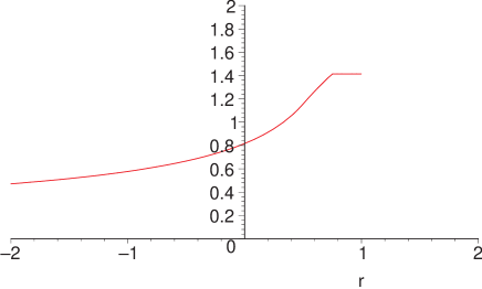
Figure 1: The von Neumann condition for the second order accurate discretization of the NOR system in 3D using 4RK as a function of the parameter $r$. For $r>1$ the scheme is unconditionally unstable.

We now restrict ourselves to the case $r=0$ and prove numerical stability. In this case the characteristic variables associated with the non trivial eigenvalues are

$$\hat{w}^{(\pm)}_{ij}=\hat{K}_{ij}\mp\frac{1}{2}i\Omega\hat{\gamma}_{ij}\pm\frac{\sin\xi_{(i}\hat{\Gamma}_{j)}}{2\chi_{2}}\,.$$ (163)

A conserved quantity is

$$E_{C} = \frac{1}{2}|\hat{w}^{(+)}_{ij}|^{2}+\frac{1}{2}|\hat{w}^{(-)}_{ij}|^{2}+a|\hat{w}_{i}^{(0)}|^{2}$$

$$= |\hat{K}_{ij}|^{2}+|s_{(i}\hat{\Gamma}_{j)}|^{2}+\frac{\Omega^{2}}{4}|\hat{\gamma}_{ij}|^{2}-{\rm Re}\left(\frac{i}{h}\sin\xi_{i}\hat{\gamma}_{ij}\overline{\hat{\Gamma}_{j}}\right)+a|\hat{\Gamma}_{i}|^{2},$$

where $2\chi_{2}s_{i}=\sin\xi_{i}$.

Since

$$|s_{i}|\leq 1$$

$$0\leq|s_{(i}\hat{\Gamma}_{j)}|^{2}\leq|s_{i}\hat{\Gamma}_{j}|^{2}\leq|\hat{\Gamma}_{i}|^{2}-\frac{4}{\varepsilon_{1}h^{2}}\chi_{2}^{2}|\hat{\gamma}_{ij}|^{2}-\varepsilon_{1}|\hat{\Gamma}_{i}|^{2}$$

$$\leq-2{\rm Re}\left(\frac{i}{h}\sin\xi_{i}\hat{\gamma}_{ij}\overline{\hat{\Gamma}_{j}}\right)\leq\frac{4}{\varepsilon_{2}h^{2}}\chi_{2}^{2}|\hat{\gamma}_{ij}|^{2}+\varepsilon_{2}|\hat{\Gamma}_{i}|^{2},$$

we have the equivalence with $|\hat{\mbox{\boldmath$u$}}|_{\Gamma}^{2}$. Inequality (154) guarantees the equivalence of the latter with $|\hat{\mbox{\boldmath$u$}}|^{2}$. This completes the proof of stability with respect to the norm

$$\left(\|\gamma_{ij}\|_{h}^{2}+\|K_{ij}\|_{h}^{2}+\|D_{+k}\gamma_{ij}\|_{h}^{2}+\|f_{i}\|_{h}^{2}\right)^{1/2}.$$ (164)

4.5 The ADM system

With a densitized lapse function, $\alpha=\det(\gamma_{ij})^{1/2}$, the ADM equations linearized about the Minkowski solution in Cartesian coordinates take the form

$$\partial_{t}\gamma_{ij} = -2K_{ij}\,,$$ (165)

$$\partial_{t}K_{ij} = \partial_{k}\partial_{(i}\gamma_{j)k}-\frac{1}{2}\partial^{k}\partial_{k}\gamma_{ij}-\partial_{i}\partial_{j}\tau\,.$$ (166)

The symbol $\hat{P}(i\omega)$ of (165)–(166) is not diagonalizable and neither is that of its differential nor its pseudo-differential reduction. The family of solutions in which the only non vanishing components are $\gamma_{1A}=\sin(\omega x)t$, $K_{1A}=-\sin(\omega x)/2$, where $A=2,3$, can be used to explicitly show instability. It gives

$$\frac{\|\mbox{\boldmath$u$}(t,\cdot)\|}{\|\mbox{\boldmath$u$}(0,\cdot)\|}=\left(1+4t^{2}+4\omega^{2}t^{2}\right)^{1/2},$$ (167)

where $\|u(t,\cdot)\|^{2}=\|\gamma_{ij}(t,\cdot)\|^{2}+\|K_{ij}(t,\cdot)\|+\|\partial_{k}\gamma_{ij}(t,\cdot)\|^{2}$. The ratio cannot be bounded by $Ke^{\alpha t}$ with $K$ and $\alpha$ independent of $\omega$.

To see that the second order accurate standard discretization is unstable we take $\gamma_{1A}=(-1)^{j}t$ and $K_{1A}=(-1)^{j+1}/2$. As in the continuum, the ratio

$$\frac{\|\mbox{\boldmath$v$}(t)\|_{h,D_{+}}}{\|\mbox{\boldmath$v$}(0)\|_{h,D_{+}}}=\left(1+4t^{2}+16\frac{t^{2}}{h^{2}}\right)^{1/2}$$ (168)

cannot be bounded. We can nevertheless compute the von Neumann condition, which is given by

$$\lambda\leq\frac{\sqrt{3}\alpha_{0}}{2\sqrt{7d}}.$$ (169)

In [26] stability tests were done with the non linear version of this formulation. The domain used consisted of a thin channel, with an even number $N$ of grid points in one spatial direction and 3 grid points in the other two directions. By taking this into account we see that modes corresponding to the frequencies $\xi_{1}=\pi$, and $\xi_{2}=\xi_{3}=2\pi/3$ grow exponentially if $\lambda>0.4163$. Figure 2 in [26] confirms that with a Courant factor of $\lambda=0.5$ there is a violation of the von Neumann condition.

Although the symbol associated with the continuum system (165) and (166) has four Jordan blocks of size two for any $\omega$, interestingly, the symbol associated with the semi-discrete problem obtained with the standard second order accurate discretization can have rather different properties. For Fourier modes traveling in directions parallel to the axis the continuum result still holds. However, for Fourier modes not parallel to any of the axis, we found that the symbol may have fewer Jordan blocks. For some Fourier frequencies we even noticed that the symbol is diagonalizable. There is no conflict between this observation and the fact that the continuum problem is ill-posed. As shown at the beginning of this subsection the discrete initial value problem for the ADM system is also ill-posed. In the limit of high resolution, $h\to 0$ ($\xi\to 0$ and $\omega$ fixed), the discrete symbol is a perturbation of the continuum one

$$\hat{P}_{d}=\hat{P}_{c}+O(h^{2}).$$

Even though for some frequencies $\hat{P}_{d}$ is diagonalizable, the characteristic variables become degenerate in the limit $h\to 0$, which implies that the discrete symmetrizer becomes unbounded (it is not possible to find a $K$, independent of $h$, satisfying inequality (103)).

4.6 The Z4 system

The same family of solutions that was used to show instability of the discretized ADM equations can be used for the standard discretization of the linearized $Z4$ system [19]

$$\partial_{t}\alpha = -f(K-m\Theta)\,,$$

$$\partial_{t}\gamma_{ij} = -2K_{ij}\,,$$

$$\partial_{t}K_{ij} = -\partial_{i}\partial_{j}\alpha-\frac{1}{2}\partial_{k}\partial_{k}\gamma_{ij}+\partial_{k}\partial_{(i}\gamma_{j)k}-\frac{1}{2}\partial_{i}\partial_{j}\tau+2\partial_{(i}Z_{j)}\,,$$

$$\partial_{t}\Theta = \frac{1}{2}(\partial_{k}\partial_{l}\gamma_{kl}-\partial_{k}\partial_{k}\tau)+\partial_{k}Z_{k}\,,$$

$$\partial_{t}Z_{i} = \partial_{k}K_{ik}-\partial_{i}K+\partial_{i}\Theta\,,$$

for any values of the parameters $f$ and $m$. This instability, however, is not present if the $D_{0}^{2}$ discretization is used as in [24], in conjunction with the $D_{0}$-norm. Furthermore, it is possible that artificial dissipation may cure this instability of the standard discretization, at least for $0<f\neq 1$ or $1=f=m/2$, since in this case the continuum Cauchy problem is well-posed. Note that while we use the same family of solutions that was used to show instability for the ADM case, the two cases are very different: While the ADM instability is due to the lack of well-posedness of the continuum equations, the problem with the Z4 system arises purely at the discrete level, and can be traced back to the difference in structure between the principal symbols of the pseudodifferential first order reductions of the continuum and discrete equations, see Eqs. (72) and (100). For second order in space systems diagonalizability of the discrete symbol is not implied by diagonalizability of the continuum symbol.

The ADM and Z4 examples suggest a simple criterion that can be used to rule out certain schemes. Any first order in time, second order in space system of PDEs which gives rise to an ill-posed problem when the first order and mixed second order spatial derivatives are dropped will result in an unstable scheme if the standard discretization is used and no artificial dissipation is added. This is a consequence of the fact that grid modes with the highest frequency belong to the kernel of the $D_{0}$ operator. Although the $D_{0}^{2}$ discretization gives stable schemes with respect to the $D_{0}$-norm, provided that the continuum problem is well-posed, it suffers from the limitations described in section 4.2.2.

5 Testing stability

When dealing with variable coefficient or non linear problems it can be difficult, if not impossible, to prove stability with respect to a certain norm. Numerical experiments are often the only option. Given a discretization of the linear initial value problem (1) and (2), a stability test should be aimed at establishing the existence of the constants $\alpha$ and $K$, independent of the initial data and for all $h\leq h_{0}$ (and possibly $k\leq\lambda_{0}h$), by computing the ratio between a suitable discrete norm at time-step $t_{n}=nk$ and its initial value,

$$\frac{\|v^{n}\|}{\|v^{0}\|}\leq Ke^{\alpha t_{n}}.$$ (170)

Although it is not possible to infer stability by examining a finite number of numerical experiments (one would have to explore the entire set $h\leq h_{0}$ that appears in the definition of stability), it is usually not difficult to spot a trend of behavior as the resolution is increased. To ensure that a wide range of frequencies is excited, random initial data can be used [27], as no smoothness assumptions are used in the definition of stability.

In the examples of first order in time, second order in space hyperbolic systems for which we are able to determine stability, we use a norm which is the discrete version of the continuum one. The derivatives are approximated using the one-sided operators $D_{+}$ (or, equivalently, $D_{-}$) rather than $D_{0}$. For the NOR system, for example, we use the square root of the expression

$$\sum_{i,j=1}^{3}\|\gamma_{ij}\|_{h}^{2}+\sum_{i,j=1}^{3}\|K_{ij}\|_{h}^{2}+\sum_{k,i,j=1}^{3}\|D_{+k}\gamma_{ij}\|_{h}^{2}+\sum_{i=1}^{3}\|f_{i}\|_{h}^{2}.$$

If, as we vary the initial data and the resolution, the experiments indicate that the constants $\alpha$ and $K$ in (170) exist, then one would conclude that the scheme appears to be stable. If not, the scheme appears to be unstable.

In the nonlinear case, if the problem has a sufficiently smooth solution $u_{0}$, then to first approximation the error equation can be linearized about $u_{0}$ and convergence follows if the linearized equation is stable (Sec. 5.5 in [20]). Establishing stability experimentally using the linearized equations would not be very practical. However, convergence to a known exact solution can be tested directly and it avoids many complications. Rather than testing for stability, one could test convergence in a more demanding way: initial data can be chosen which is not smooth, but is accurate to the correct order in the appropriate norm. For instance, for the NOR system, one would use the square root of

$$\sum_{i,j=1}^{3}\|\delta\gamma_{ij}\|_{h}^{2}+\sum_{i,j=1}^{3}\|\delta K_{ij}\|_{h}^{2}+\sum_{k,i,j=1}^{3}\|D_{+k}(\delta\gamma_{ij})\|_{h}^{2}+\sum_{i=1}^{3}\|\delta f_{i}\|_{h}^{2},$$

where $\delta v=v-u_{0}$, and one could add random noise to the initial data with amplitude $h^{p}$ for the $K_{ij}$ and $f_{i}$ variables and $h^{p+1}$ for the $\gamma_{ij}$ variables. The scheme is convergent around the solution $u_{0}$ if the $D_{+}$-norm of the error at time $T$ is of order $h^{p}$. In particular, this implies that for a convergent scheme the discrete $L_{2}$ norm of the error is of order $h^{p}$ if the $D_{+}$-norm of the initial error is of order $h^{p}$.

Finally, we note that the notion of robust stability introduced in [27] does not imply nor follows from the concept of numerical stability investigated in this paper.

5.1 Numerical tests

We have performed numerical tests to complement the analytical stability results of Sec. 4.

For each run, the numerical grid has dimensions $50\rho\times 4\times 4$, where $\rho=1,2,4,8$ parameterizes the resolution, and we impose periodic boundary conditions. The coordinate domain is $x,y,z\in[-0.5,0.5)$. The time integrator is RK4 with Courant factor $\lambda=0.5$. We choose random noise of order unity as initial data (except for the Z4 tests, see below) so that many discrete Fourier modes are present in the initial data. Empirically, we find that using smooth initial data in the constant coefficient problems of this paper can make it difficult to observe an instability. This was also noticed in the nonlinear case in [28].

Figure 2 shows the results for the ADM system. The apparent trend is that as the resolution is increased, and higher frequency Fourier modes are present in the initial data, the ratio of the $D_{+}$-norm of the solution to its initial value at any given time increases. It appears that there is no $K,\alpha$ such that this quantity can be bounded by a function $Ke^{\alpha t_{n}}$, and this indicates that the system is unstable.

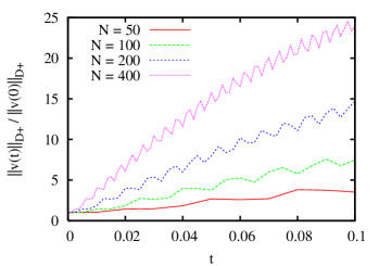
Figure 2: Linearized ADM stability test

In Figure 3 we show the results of the stability test for the linearized NOR system. The results suggest that the ratio of the $D_{+}$-norm of the solution to its initial value remains bounded, and hence that the system is stable. This reflects the analytic result that we proved in Sec. 4.

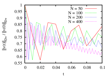
Figure 3: Linearized NOR stability test, $r=0$

Showing the instability of the Z4 system was more complicated. In this case, it was not sufficient to use random initial data of order unity in all variables. When this was attempted, the ratio of the $D_{+}$-norm to its initial value remained bounded. In order to numerically demonstrate the instability, we used knowledge of the exact solution that violates the estimate. Random data of order unity was given to the variables $K_{22}$ and $K_{33}$ and the remaining variables were set to zero. The test results for the linearized Z4 system are shown in Figure 4, and confirm that this system is unstable.

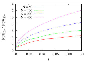
Figure 4: Linearized Z4 stability test, $f=1,m=2$. Initial data consists of random values in $K_{22}$ and $K_{33}$, and all other variables are zero.

When artificial dissipation with $\sigma=0.02$ is used, the linearized Z4 system tested with the same initial data shows no sign of instability. See Figure 5.

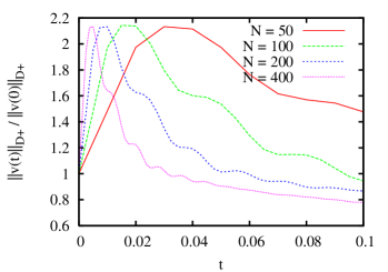
Figure 5: Linearized Z4 stability test with dissipation $\sigma=0.02$, $f=1,m=2$. Initial data consists of random values in $K_{22}$ and $K_{33}$, and all other variables are zero.

The example of the Z4 system shows that numerical testing of stability is not always straightforward, and that schemes which appear stable for simple test cases may in fact be unstable. All tests were done using the standard second order accurate discretization.

6 Discussion

In this work we extended the notion of numerical stability of finite difference approximations to include hyperbolic systems that are first order in time and second order in space. We considered the standard discretization of the wave equation, a generalization of the KWB formulation of electromagnetism and the NOR formulation of Einstein’s equations linearized about the Minkowski solution. By analyzing the symbol of the second order system, and constructing a discrete symmetrizer, we were able to prove stability in a discrete norm containing one-sided difference operators, provided that the von Neumann condition is satisfied. Consistency and stability with respect to the $D_{+}$-norm imply convergence with respect to the discrete $L_{2}$ norm. We also found that in some cases ($r\geq 1$ in the NOR and generalized KWB systems, and Z4) standard discretizations of well-posed continuum problems can lead to unconditionally unstable schemes. This is closely related to the instability of the fully second order shifted wave equation investigated in [29], but our examples contain no shift terms.

Our analysis of discretizations of first order in time hyperbolic systems shows that in the first order in space case there is a clear correspondence between strong hyperbolicity and numerical stability, and between characteristic speeds and Courant limits. See inequality (113) and Eq. (114). In the second order in space case, on the other hand, the mixing of $D_{\pm}$ and $D_{0}$ operators breaks this correspondence. To restore the correspondence one could use the $D_{0}^{2}$ discretization, however, as discussed in Sec. 4.2.2, this can lead to difficulties.

In Sec. 4.6 we propose a simple criterion that can be used to rule out certain schemes when the standard discretization is used and no artificial dissipation is added. This criterion detects schemes in which the highest frequency mode grows faster as the resolution is increased.

We also discuss stability tests for second order in space systems. These tests should be aimed at establishing the existence, for sufficiently small $h$, of the constants $K$ and $\alpha$ that appear in the definition of stability with respect to the $D_{+}$-norm. In the nonlinear case the situation is more complicated. In this case we suggest, when an exact smooth solution of the continuum problem is available, to do convergence tests with initial data given by that of the continuum problem plus random noise of order $h^{p}$ with respect to the $D_{+}$-norm (see Sec. 5).

Although our analysis was restricted to the constant coefficient case, we expect that for the variable coefficient case generalizations of results similar to those presented in Sec. 6.6 of [20] for first order hyperbolic systems, where artificial dissipation plays an important role, might apply.

7 Acknowledgments

We wish to thank Carsten Gundlach and Olivier Sarbach for helpful discussions and suggestions. This research was supported by a Marie Curie Intra-European Fellowship within the 6th European Community Framework Program.

Appendix A Time integrators

In this work we restrict our attention to the following three time integrators: 3rd and 4th order Runge-Kutta, and iterative Crank-Nicholson [30]. Given a system of ordinary differential equations, $dy/dt=f(t,y(t))$, these integrators are defined as

• $$k_{1} = kf(t_{n},y^{n})$$

  $$k_{2} = kf(t_{n}+k/2,y^{n}+k_{1}/2)$$

  $$k_{3} = kf(t_{n}+3k/4,y^{n}+3k_{2}/4)$$

  $$y^{n+1} = y^{n}+(2k_{1}+3k_{2}+4k_{3})/9$$

• $$k_{1} = kf(t_{n},y^{n})$$

  $$k_{2} = kf(t_{n}+k/2,y^{n}+k_{1}/2)$$

  $$k_{3} = kf(t_{n}+k/2,y^{n}+k_{2}/2)$$

  $$k_{4} = kf(t_{n}+k,y^{n}+k_{3})$$

  $$y^{n+1} = y^{n}+(k_{1}+2k_{2}+2k_{3}+k_{4})/6$$

• $$k_{1} = kf(t_{n},y^{n})$$

  $$k_{2} = kf(t_{n}+k/2,y^{n}+k_{1}/2)$$

  $$k_{3} = kf(t_{n}+k/2,y^{n}+k_{2}/2)$$

  $$y^{n+1} = y^{n}+k_{3}$$

Appendix B Some numerical properties of first and second order systems

In this section we assume that the time integrator is one of those discussed in Appendix A. We consider standard second and fourth order accurate discretizations of the following two toy model problems

$$u_{t}=u_{x}\,,$$ (171)

and

$$\phi_{t}=\Pi\,,\qquad\Pi_{t}=\phi_{xx}\,.$$ (172)

Eq. (171) arises in the full reduction to first order of $\phi_{tt}=\phi_{xx}$, while (172) represents its reduction in time. If we denote by $\lambda(\xi)$ an eigenvalue of the discrete symbol, the corresponding phase and group velocities are given by

$$v_{\rm p} = i\frac{\lambda(\xi)}{\omega}\,,$$

$$v_{\rm g} = i\frac{d}{d\omega}\lambda(\xi)\,,$$

where $\xi=\omega h$. In the following table we compute the numerical phase velocities, $v_{\rm p}$, group velocities, $v_{\rm g}$, the Courant limits (C.l.), the frequencies of undamped modes (u.m.) and of the first unstable mode (f.u.m.) for the two systems. The numerical phase and group velocities are plotted in Figure 6 as a function of $\xi$.

In the table we used $\Delta^{2}=1+\frac{1}{3}\sin^{2}\frac{\xi}{2}$. The exact continuum phase and group velocity is 1. The Taylor expansion of the numerical velocities gives an idea of the magnitude of the error, provided that enough grid-points per wave length are used. The table shows that in the second order accurate case the phase error for the wave equation is 4 times smaller than for the advective equation, and that this improvement in accuracy is even stronger for the fourth order accurate discretization.

Furthermore, the standard discretizations of fully first order hyperbolic systems have numerical phase velocities that vanish at the highest frequencies and numerical group velocities with the opposite sign to the continuum one. In numerical relativity simulations involving black holes which make use of the excision technique to handle the singularity one can expect to see numerical high frequency solutions escaping from the black hole, if a first order formulation combined with the standard discretization is used, unless artificial dissipation is added to the scheme.

Finally, whereas for (171) the transition from second order accuracy to fourth order implies the reduction of the Courant limit by a factor of $1.372$, for the second order in space system (172), this transition requires a Courant limit $2/\sqrt{3}\approx 1.155$ times smaller. This indicates that there is an even higher gain in going to fourth order accuracy for second order in space formulations.

	2nd order accurate		4th order accurate
	advective	wave	advective	wave
$v_{\rm p}$	$\begin{array}[]{c}\frac{\sin\xi}{\xi}\approx\\ 1-\frac{\xi^{2}}{6}+O(\xi^{4})\end{array}$	$\begin{array}[]{c}\frac{2}{\xi}\sin\frac{\xi}{2}\approx\\ 1-\frac{\xi^{2}}{24}+O(\xi^{4})\end{array}$	$\begin{array}[]{c}\frac{\sin\xi}{\xi}\left(1+\frac{2}{3}\sin^{2}\frac{\xi}{2}\right)\\ \approx 1-\frac{\xi^{4}}{30}+O(\xi^{6})\end{array}$	$\begin{array}[]{c}\frac{2}{\xi}\sin\frac{\xi}{2}\Delta\approx\\ 1-\frac{\xi^{4}}{180}+O(\xi^{6})\end{array}$
$v_{\rm g}$	$\begin{array}[]{c}\cos\xi\approx\\ 1-\frac{\xi^{2}}{2}+O(\xi^{4})\end{array}$	$\begin{array}[]{c}\cos\frac{\xi}{2}\approx\\ 1-\frac{\xi^{2}}{8}+O(\xi^{4})\end{array}$	$\begin{array}[]{c}1-\frac{8}{3}\sin^{4}\frac{\xi}{2}\approx\\ 1-\frac{\xi^{4}}{6}+O(\xi^{6})\end{array}$	$\begin{array}[]{c}\cos\frac{\xi}{2}\left(1+\frac{2}{3}\sin^{2}\frac{\xi}{2}\right)/\Delta\\ \approx 1-\frac{\xi^{4}}{36}+O(\xi^{6})\end{array}$
C.l.	$\alpha_{0}$	$\alpha_{0}/2$	$\alpha_{0}/1.372$	$\frac{\sqrt{3}}{4}\alpha_{0}\approx\alpha_{0}/2.309$
u.m.	$0,\pi$	$0$	$0,\pi$	$0$
f.u.m.	$\pm\frac{\pi}{2}\approx\pm 1.571$	$\pi$	$\begin{array}[]{c}\pm 2\arctan\left(\frac{6^{1/4}}{\sqrt{4-\sqrt{6}}}\right)\\ \approx\pm 1.797\end{array}$	$\pi$

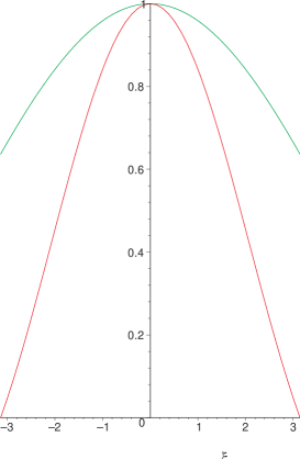
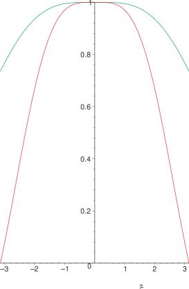
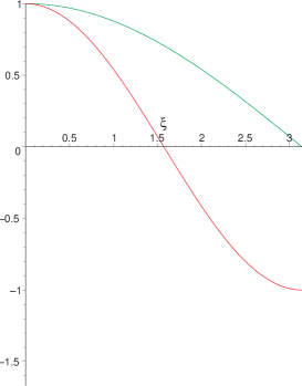
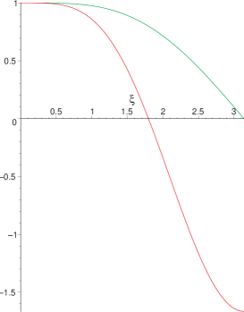
Figure 6: The phase (top) and group (bottom) velocities for the second (left) and fourth (right) order standard approximation of the advective equation (171) (red) and the wave equation (172) (green).

Appendix C Discrete constraint propagation

When simulating systems such as Maxwell’s or Einstein’s equations, one has to take into account that the data has to satisfy initial data constraints. The evolution equations guarantee that if these constraints are satisfied initially, then they will be satisfied at later times. In this appendix we show that even in the constant coefficient case, when using standard discretizations of second order in space systems, the discrete constraints do not propagate exactly. Initial data which satisfy the discrete constraints do not lead to constraint satisfying solutions.

As an example, we consider the ADM equations (165)–(166) with constraints

$$C\equiv\frac{1}{2}(\partial_{i}\partial_{j}\gamma_{ij}-\partial_{i}\partial_{i}\tau)=0\,,\qquad C_{i}\equiv\partial_{j}K_{ij}-\partial_{i}K=0\,.$$

For simplicity we confine ourselves to solutions which depend only on one space coordinate. The discretized constraints are

$$C\equiv-\frac{1}{2}D_{+}D_{-}\gamma_{AA}=0\,,\qquad C_{1}\equiv-D_{0}K_{AA}=0\,,$$

$$C_{A}\equiv D_{0}K_{1A}=0\,,$$

where $A=2,3$.

The time derivative of the first constraint cannot be expressed in terms of finite difference combinations of the constraints

$$\frac{d}{dt}C=D_{+}D_{-}K_{AA}\neq-D_{0}C_{1}\,.$$

This is to be contrasted with the fact that in the constant coefficient case, the discrete constraints of a first order reduction would propagate as in the continuum, with partial derivatives replaced by $D_{0}$ operators. Furthermore, this issue would not be present if one used $D_{0}^{2}$ to approximate the second derivatives.

References

- [1] M. Shibata and T. Nakamura, Phys. Rev. D 52, 5428 (1995).
- [2] T. Baumgarte and S. Shapiro, Phys. Rev. D 59, 024007 (1999).
- [3] S. Frittelli and O. Reula, Phys. Rev. Lett. 76, 4667 (1996).
- [4] S.D. Hern, Ph.D. Thesis, University of Cambridge, 1999, gr-qc/0004036.
- [5] A. Anderson and J.W. York, Jr., Phys. Rev. Lett. 82, 4384 (1999).
- [6] L.E. Kidder, M.A. Scheel, and S.A. Teukolsky, Phys. Rev. D 64, 064017 (2001).
- [7] O. Sarbach, G. Calabrese, J. Pullin, and M. Tiglio, Phys. Rev. D 66, 064002 (2002).
- [8] G. Nagy, O. Ortiz, and O. Reula, Phys. Rev. D 70, 044012 (2004)
- [9] C. Gundlach, J.M. Martin-Garcia, Phys. Rev. D 70, 044031 (2004).
- [10] C. Gundlach, J.M. Martin-Garcia, Phys. Rev. D 70, 044032 (2004).
- [11] H. Beyer and O. Sarbach, Phys. Rev. D 70, 104004 (2004).
- [12] H. Kreiss, N. Petersson, and J. Yström, SIAM J. Numer. Anal. 40, 1940-1967 (2002).
- [13] B. Szilágyi, H.-O. Kreiss, and J. Winicour, Phys. Rev. D 71, 104035 (2005).
- [14] R.D. Richtmyer and K. Morton, Difference Methods for Initial Value Problems (Interscience Publisher, New York, 1967).
- [15] S. Frittelli and R. Gómez, J. Math. Phys. 41 5535 (2000).
- [16] A. Knapp, E. Walker and T. Baumgarte, Phys. Rev. D 65, 064031 (2002).
- [17] C. Nunn, M.Phil. Thesis, University of Southampton, 2005.
- [18] R. Arnowitt, S. Deser, and C. Misner, in Gravitation: An Introduction to Current Research, edited by L. Witten (Wiley, New York, 1962).
- [19] C. Bona, T. Ledvinka, C. Palenzuela, and M. Žáček, Phys. Rev. D 67, 104005 (2003).
- [20] B. Gustafsson, H.-O. Kreiss, and J. Oliger, Time dependent problems and difference methods (John Wiley & Sons, New York, 1995).
- [21] H.-O. Kreiss, J. Lorenz, Initial-Boundary Value Problems and the Navier-Stokes Equations (Academic Press, Boston, 1989).
- [22] H.-O. Kreiss and G. Scherer, SIAM J. Numer. Anal., 29, No. 3, 640-646 (1992).
- [23] H.-O. Kreiss and O.E. Ortiz, in Lecture Notes in Physics 604 (Springer, New York, 2002).
- [24] C. Bona, T. Ledvinka, C. Palenzuela, and M. Žáček, Phys. Rev. D 69, 064036 (2004).
- [25] M. Babiuc, B. Szilágyi, and J. Winicour, gr-qc/0404092.
- [26] M. Alcubierre et al., Class. Quantum Grav. 21 589 (2004).
- [27] B. Szilágyi, R. Gómez, N.T. Bishop, J. Winicour, Phys. Rev. D 62 104006 (2000).
- [28] G. Calabrese, J. Pullin, O. Sarbach and M. Tiglio, Phys. Rev. D 66, 064011 (2002).
- [29] G. Calabrese, Phys. Rev. D 71, 027501 (2005).
- [30] S.A. Teukolsky, Phys. Rev. D 61, 087501 (2000).