Semiclassical approach to black hole absorption of electromagnetic radiation emitted by a rotating charge

Abstract

We consider an electric charge, minimally coupled to the Maxwell field, rotating around a Schwarzschild black hole. We investigate how much of the radiation emitted from the swirling charge is absorbed by the black hole and show that most of the photons escape to infinity. For this purpose we use the Gupta-Bleuler quantization of the electromagnetic field in the modified Feynman gauge developed in the context of quantum field theory in Schwarzschild spacetime. We obtain that the two photon polarizations contribute quite differently to the emitted power. In addition, we discuss the accurateness of the results obtained in a full general relativistic approach in comparison with the ones obtained when the electric charge is assumed to be orbiting a massive object due to a Newtonian force.

I Introduction

Much effort has been devoted to confirm the presence of black holes in X-ray binary systems evid1 as well as in galactic centers evid2 . The analysis of the radiation emitted from accretion disks swirling around black hole candidates may play a crucial role in the experimental confirmation of the existence of event horizons (see, e.g., Ref. accdisks ). It is interesting, thus, to compute the amount of the emitted radiation which is able to reach asymptotic observers rather than be absorbed by the hole. In a recent work, Higuchi and two of the authors analyzed the radiation emitted by a scalar source rotating around a Schwarzschild black hole CHM2CQG . In the present work we study the more realistic case where the scalar source is replaced by an electric charge. In order to capture the full influence of the spacetime curvature on the emitted radiation, we work in the context of quantum field theory in Schwarzschild spacetime (for a comprehensive account on quantum field theory in curved spacetimes see, e.g., Ref. BD ). Because of the difficulty to express the solution of some differential equations which we deal with in terms of known special functions (see e.g. Ref. Candetal for a discussion on this issue) our computations are performed (i) numerically but without further approximations and (ii) analytically but restricted to the low-frequency regime (in which case the radial part of the normal modes can be written in terms of Legendre functions GR ).

We organize the paper as follows. In Section II we review the Gupta-Bleuler quantization of the electromagnetic field in a modified Feynman gauge in the spacetime of a static chargeless black hole CHM3PRD . We compute the radiated power from an electric charge swirling around a Schwarzschild black hole in Section III. In Section IV we compare this result with the one obtained considering the charge as orbiting a Newtonian object in flat spacetime. Finally we use the previous results to compute in Section V what is the amount of the emitted radiation which is able to reach asymptotic observers. Our final remarks are made in Section VI. We assume natural units $\hbar=c=G=1$ and metric signature $(+---)$.

II Quantization of the electromagnetic field in Schwarzschild spacetime

In this section we review the quantization of the massless vector field in Schwarzschild spacetime following closely Ref. CHM3PRD . We write the line element of a static chargeless black hole as

$$ds^{2}=f\left(r\right)dt^{2}-f\left(r\right)^{-1}dr^{2}-r^{2}d\theta^{2}-r^{2}\sin^{2}\theta d\phi^{2}\,,$$ (1)

where $f\left(r\right)=1-2M/r$.

We then consider a massless vector field in this geometry with classical action given by

$$S=\int d^{4}x\mathcal{L}\,,$$ (2)

where the Lagrangian density in the modified Feynman gauge is

$$\mathcal{L}=\sqrt{-g}\left[-\dfrac{1}{4}F_{\mu\nu}F^{\mu\nu}-\dfrac{1}{2}G^{2}\right]$$ (3)

with $g=r^{2}\sin\theta$, $G\equiv\nabla^{\mu}A_{\mu}+K^{\mu}A_{\mu}$ and

$$K^{\mu}=\left(0,{df}/{dr},0,0\right)\text{.}$$

The corresponding Euler-Lagrange equations are, thus,

$$\nabla_{\nu}F^{\mu\nu}+\nabla^{\mu}G-K^{\mu}G=0\text{,}$$ (4)

which can be cast in the form

$$\dfrac{1}{f}\partial_{t}^{2}A_{t}-\dfrac{f}{r^{2}}\partial_{r}\left(r^{2}\partial_{r}A_{t}\right)+\dfrac{1}{r^{2}}\tilde{\nabla}^{2}A_{t}~{}=0\,,$$ (5)

$$\dfrac{1}{f}\partial_{t}^{2}A_{r}-\dfrac{1}{f}\partial_{r}\left[\dfrac{f^{2}}{r^{2}}\partial_{r}\left(r^{2}A_{r}\right)\right]+\dfrac{1}{r^{2}}\tilde{\nabla}^{2}A_{r}$$

$$+\dfrac{1}{f}\partial_{r}\left(\dfrac{f}{r^{2}}\right)\tilde{\nabla}^{a}A_{a}=0\,,$$ (6)

$$\dfrac{1}{f}\partial_{t}^{2}A_{a}-\partial_{r}\left(f~{}\partial_{r}A_{a}\right)+\dfrac{1}{r^{2}}\left[\tilde{\nabla}^{b}\left(\tilde{\nabla}_{b}A_{a}-\tilde{\nabla}_{a}A_{b}\right)\right.$$

$$\left.+\partial_{a}\tilde{\nabla}^{b}A_{b}\right]+r^{2}\partial_{r}\left(\dfrac{f}{r^{2}}\right)\partial_{a}A_{r}=0\,.$$ (7)

Here $a$ and $b$ denote angular variables on the unit $2$-sphere $S^{2}$ with metric $\tilde{\eta}_{ab}$ and inverse metric $\tilde{\eta}^{ab}$ [with signature $(--)]$, $\tilde{\nabla}_{a}$ is the associated covariant derivative on $S^{2}$, $\tilde{\nabla}^{a}\equiv\tilde{\eta}^{ab}\tilde{\nabla}_{b}$ and $\tilde{\nabla}^{2}\equiv\tilde{\eta}_{ab}\tilde{\nabla}^{a}\tilde{\nabla}^{b}$.

We write the complete set of positive-frequency solutions of Eq. (4) with respect to the Killing field $\partial_{t}$ in the form

$$A^{(\varepsilon n\omega lm)}_{\mu}=\zeta^{\varepsilon n\omega lm}_{\mu}(r,\theta,\phi)e^{-i\omega t},\,\,\,\,\,\omega>0.$$ (8)

The index $\varepsilon$ stands for the four different polarizations. The pure gauge modes, $\varepsilon={\rm G}$, are the ones which satisfy the gauge condition $G=0$ and can be written as $A^{({\rm G}n\omega lm)}_{\mu}=\nabla_{\mu}\Lambda$, where $\Lambda$ is a scalar field. The physical modes, $\varepsilon={\rm I},{\rm II}$, satisfy the gauge condition and are not pure gauge. The nonphysical modes, $\varepsilon={\rm NP}$, do not satisfy the gauge condition. The modes incoming from the past null infinity ${\cal J}^{-}$ are denoted by $n=\leftarrow$ and the modes incoming from the past event horizon $H^{-}$ are denoted by $n=\rightarrow$. The $l$ and $m$ are the angular momentum quantum numbers.

The physical modes can be written as

$$A_{\mu}^{({\rm I}n\omega lm)}=\left(0\,,\,\dfrac{{\varphi}_{\omega l}^{{\rm I}n}\left(r\right)}{r}~{}Y_{lm},\dfrac{f}{l\left(l+1\right)}\dfrac{d}{dr}\left[r{\varphi}_{\omega l}^{{\rm I}n}\left(r\right)\right]\partial_{\theta}Y_{lm},\dfrac{f}{l\left(l+1\right)}\dfrac{d}{dr}\left[r{\varphi}_{\omega l}^{{\rm I}n}\left(r\right)\right]\partial_{\phi}Y_{lm}\right)e^{-i\omega t}$$ (9)

and

$$A_{\mu}^{({\rm II}n\omega lm)}=\left(0,0,r{\varphi}_{\omega l}^{{\rm II}n}\left(r\right)Y_{\theta}^{lm},r{\varphi}_{\omega l}^{{\rm II}n}\left(r\right)Y_{\phi}^{lm}\right)e^{-i\omega t}$$ (10)

with $l\geqslant 1$ (since the gauge condition $G=0$ is not satisfied for $l=0$). The radial part of the physical modes satisfies the differential equation

$$\left(\omega^{2}-V_{S}\right)\left[r{\varphi}_{\omega l}^{\lambda n}\left(r\right)\right]+f\dfrac{d}{dr}\left(f\dfrac{d}{dr}\left[r{\varphi}_{\omega l}^{\lambda n}\left(r\right)\right]\right)=0\text{,}$$ (11)

where $\lambda={\rm I},{\rm II}$ and

$$V_{S}=\left(1-\dfrac{2M}{r}\right)\dfrac{l\left(l+1\right)}{r^{2}}$$ (12)

is the Schwarzschild scattering potential (see solid line in Fig. 1). $Y_{lm}$ and $Y_{a}^{lm}$ are scalar and vector spherical harmonics AHCQG , respectively. The remaining modes can be written as

$$A_{\mu}^{({\rm NP}n\omega lm)}=\left({\varphi}_{\omega l}^{{\rm NP}n}\left(r\right)Y_{lm},0,0,0\right)e^{-i\omega t}$$ (13)

and

$$A_{\mu}^{({\rm G}n\omega lm)}=\nabla_{\mu}\Lambda^{\omega nlm}$$ (14)

with $l\geqslant 0$, where

$$\Lambda^{\omega nlm}=\dfrac{i}{\omega}{\varphi}_{\omega l}^{{\rm NP}n}\left(r\right)Y_{lm}e^{-i\omega t}$$

and ${\varphi}_{\omega l}^{{\rm NP}n}$ satisfies

$$\left(\omega^{2}-V_{S}\right){\varphi}_{\omega l}^{{\rm NP}n}\left(r\right)+\dfrac{f^{2}}{r^{2}}\dfrac{d}{dr}\left(r^{2}\dfrac{d}{dr}{\varphi}_{\omega l}^{{\rm NP}n}\left(r\right)\right)=0\text{.}$$ (15)

The conjugate momenta associated with the field modes are defined by

$$\Pi^{(i)\mu\nu} \equiv \left.\dfrac{1}{\sqrt{-g}}\dfrac{\partial\mathcal{L}}{\partial\left[\nabla_{\mu}A_{\nu}\right]}\right|_{A_{\mu}=A^{(i)}_{\mu}}$$ (16)

$$= -\left.\left[F^{\mu\nu}+g^{\mu\nu}G\right]\right|_{A_{\mu}=A^{(i)}_{\mu}}\text{,}$$

where $(i)$ represents $(\varepsilon,n,\omega,l,m)$. By writing the conserved current

$$W^{\mu}\left[A^{(i)},A^{(j)}\right]\equiv i\left[\overline{A_{\nu}^{(i)}}\Pi^{(j)\mu\nu}-\overline{\Pi^{(i)\mu\nu}}A_{\nu}^{(j)}\right]\,,$$ (17)

where the overline denotes complex conjugation, we normalize the field modes through the generalized Klein-Gordon inner product CHM defined by

$$\left(A^{(i)},A^{(j)}\right)\equiv\int_{\Sigma}d\Sigma_{\mu}^{\left(3\right)}W^{\mu}\left[A^{(i)},A^{(j)}\right]\text{.}$$ (18)

Here $d\Sigma_{\mu}^{\left(3\right)}\equiv d\Sigma^{\left(3\right)}~{}n_{\mu}$, where $d\Sigma^{\left(3\right)}$ is the invariant 3-volume element of the Cauchy surface $\Sigma$ and $n^{\mu}$ is the future pointing unit vector orthogonal to $\Sigma$. The modes are then normalized such that

$$\left(A^{(\varepsilon n\omega lm)},A^{(\varepsilon^{\prime}n^{\prime}\omega^{\prime}l^{\prime}m^{\prime})}\right)=M^{\varepsilon\varepsilon^{\prime}}\delta_{nn^{\prime}}\delta_{ll^{\prime}}\delta_{mm^{\prime}}\delta\left(\omega-\omega^{\prime}\right)\text{,}$$ (19)

where the matrix $M^{\varepsilon\varepsilon^{\prime}}$ is given by

$$M^{\varepsilon\varepsilon^{\prime}}=\left(\begin{array}[c]{cccc}1&0&0&0\\ 0&1&0&0\\ 0&0&0&-1\\ 0&0&-1&-1\end{array}\right)$$ (20)

with $\varepsilon=({\rm I},{\rm II},{\rm G},{\rm NP})$.

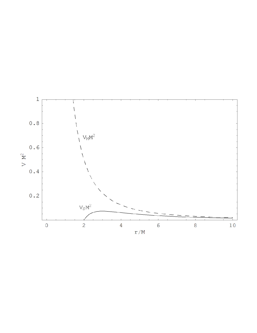
Figure 1: The potentials $V_{S}$ (solid line) and $V_{M}$ (dashed line), for $l=1$, are plotted as a function of $r/M$ with $r$ being the radial coordinate in Schwarzschild and Minkowski spacetimes, respectively. The Schwarzschild potential is restricted to $r>2M$ while for the Minkowski potential we have $r>0$. Note that both $V_{S}$ and $V_{M}$ decrease asymptotically as $1/r^{2}$ but behave quite differently for $r\approx 2M$.

In order to quantize the electromagnetic field, we demand the equal time commutation relations

$$\left[\hat{A}_{\mu}\left(\mathbf{x},t\right),\hat{A}_{\nu}\left(\mathbf{x}^{\prime},t\right)\right]=\left[\hat{\Pi}_{\mu t}\left(\mathbf{x},t\right),\hat{\Pi}_{\nu t}\left(\mathbf{x}^{\prime},t\right)\right]=0\text{,}$$ (21)

$$\left[\hat{A}_{\mu}\left(\mathbf{x},t\right),\hat{\Pi}^{t\nu}\left(\mathbf{x}^{\prime},t\right)\right]=\dfrac{i\delta_{\mu}^{\nu}}{\sqrt{-g}}\delta^{3}\left(\mathbf{x}-\mathbf{x}^{\prime}\right)\text{.}$$ (22)

The electromagnetic field operator can be expanded in terms of the normal modes as

$$\hat{A}_{\mu}=\sum_{\varepsilon,n,l,m}\int_{0}^{\infty}d\omega\left[\hat{a}_{(i)}A_{\mu}^{(i)}+\hat{a}_{{(i)}}^{\dagger}\overline{A_{\mu}^{(i)}}\right]\,,$$ (23)

where $\hat{a}_{(i)}$ and $\hat{a}_{{(i)}}^{\dagger}$ are the annihilation and creation operators, respectively, satisfying

$$\left[\hat{a}_{(\varepsilon n\omega lm)},\hat{a}^{\dagger}_{(\varepsilon^{\prime}n^{\prime}\omega^{\prime}l^{\prime}m^{\prime})}\right]\!\!=\!(M^{-1})_{\varepsilon\varepsilon^{\prime}}\delta_{nn^{\prime}}\delta_{ll^{\prime}}\delta_{mm^{\prime}}\delta\left(\omega-\omega^{\prime}\right).$$ (24)

The Fock space of the physical states $\left|{\rm PS}\right\rangle$ is obtained by imposing the Gupta-Bleuler condition IZ . In our case, this corresponds to impose

$$\hat{G}^{\left(+\right)}\left|{\rm PS}\right\rangle=0\text{,}$$ (25)

where $\hat{G}^{\left(+\right)}$ is the positive-frequency part of the operator $\hat{G}=\nabla^{\mu}\hat{A}_{\mu}+K^{\mu}\hat{A}_{\mu}$. Condition (25) corresponds to

$$\hat{a}_{\left({\rm NP}\omega nlm\right)}\left|{\rm PS}\right\rangle=0\text{.}$$ (26)

The physical states are obtained by applying any number of creation operators $\hat{a}^{\dagger}_{({\rm I}n\omega lm)}$, $\hat{a}^{\dagger}_{({\rm II}n\omega lm)}$ and $\hat{a}^{\dagger}_{({\rm NP}n\omega lm)}$ to the Boulware vacuum $\left|0\right\rangle$ Boul defined by

$$\hat{a}_{\left(\varepsilon n\omega lm\right)}\left|0\right\rangle=0\text{.}$$ (27)

The creation operators associated with pure gauge modes take physical states into nonphysical ones. Moreover physical states of the form $\hat{a}^{\dagger}_{({\rm NP}n\omega lm)}\left|{\rm PS}\right\rangle$ have zero norm. Therefore we can take as the representative elements of the Fock space those states obtained by applying the creation operators associated with the two physical modes to the Boulware vacuum. For this reason we will be concerned only with the two physical modes, $\lambda={\rm I},{\rm II}$, in the rest of the paper. (A more detailed discussion of the Gupta-Bleuler quantization of the electromagnetic field in spherically symmetric and static spacetimes can be found in Ref. CHM3PRD .)

The solutions of Eq. (11) are functions whose properties are not well known. (See Ref. Candetal for some properties.) We can, however, obtain their analytic form (i) in the asymptotic regions for any frequency and (ii) everywhere if we keep restricted to the low-frequency regime. In order to study the asymptotic behavior of the physical modes we use the Wheeler coordinate $x=\allowbreak r+2M\ln\left({r}/{2M}-1\right)$ and rewrite Eq. (11) as

$$\left(\omega^{2}-V_{S}\right)[r{\varphi}_{\omega l}^{\lambda n}\left(x\right)]+\dfrac{d^{2}}{dx^{2}}\left[r{\varphi}_{\omega l}^{\lambda n}\left(x\right)\right]=0\text{.}$$ (28)

Since the Schwarzschild potential (12) vanishes for $r=2M$ and decreases as $1/r^{2}$ for $r\gg 2M$ (see Fig. 1), the solutions of Eq. (28) can be approximated in the asymptotic regions by

$$r{\varphi}_{\omega l}^{\lambda\rightarrow}\left(r\right)\approx\left\{\begin{array}[c]{c}B_{\omega l}^{\lambda\rightarrow}\left(e^{i\omega x}+R_{\omega l}^{\lambda\rightarrow}e^{-i\omega x}\right)\\ B_{\omega l}^{\lambda\rightarrow}T_{\omega l}^{\lambda\rightarrow}i^{l+1}\omega xh_{l}^{\left(1\right)}\left(\omega x\right)\end{array}\right.\begin{array}[c]{c}\left(x\ll-1\right)\text{,}\\ \left(x\gg 1\right)\text{,}\end{array}$$ (29)

and

$$r{\varphi}_{\omega l}^{\lambda\leftarrow}\left(r\right)\approx\left\{\begin{array}[c]{c}B_{\omega l}^{\lambda\leftarrow}T_{\omega l}^{\lambda\leftarrow}e^{-i\omega x}\\ B_{\omega l}^{\lambda\leftarrow}\left(\left(-i\right)^{l+1}\omega xh_{l}^{\left(1\right)\ast}\left(\omega x\right)\right.\\ \left.+R_{\omega l}^{\lambda\leftarrow}i^{l+1}\omega xh_{l}^{\left(1\right)}\left(\omega x\right)\right)\end{array}\right.\begin{array}[c]{c}\left(x\ll-1\right)\text{,}\\ \\ \\ \left(x\gg 1\right)\text{,}\end{array}$$ (30)

where $r{\varphi}_{\omega l}^{\lambda\rightarrow}\left(r\right)$ and $r{\varphi}_{\omega l}^{\lambda\leftarrow}\left(r\right)$ are solutions incoming from $H^{-}$ and ${\cal J}^{-}$, respectively. Here $h_{l}^{\left(1\right)}(x)$ is a spherical Bessel function of the third kind Abramo , $B_{\omega l}^{\lambda n}$ are normalization constants, and $\left|R_{\omega l}^{\lambda n}\right|^{2}~{}\text{and }\left|T_{\omega l}^{\lambda n}\right|^{2}$ are the reflexion and transmission coefficients, respectively, satisfying the usual probability conservation equation $\left|R_{\omega l}^{\lambda n}\right|^{2}+\left|T_{\omega l}^{\lambda n}\right|^{2}=1$. Using the generalized Klein-Gordon inner product defined above we obtain

$$\left|B_{\omega l}^{{\rm I}n}\right|=\sqrt{\dfrac{l\left(l+1\right)}{4\pi}}\,\omega^{-3/2}$$ (31)

and

$$\left|B_{\omega l}^{{\rm II}n}\right|=\dfrac{1}{\sqrt{4\pi}}\,\omega^{-1/2}\,\,\text{.}$$ (32)

Let us now find the analytic expressions of the physical modes in the low-frequency approximation. For this purpose we rewrite Eq. (11) as

$$\dfrac{d}{dz}\left[\left(1-z^{2}\right)\dfrac{d{\varphi}_{\omega l}^{\lambda n}\left(z\right)}{dz}\right]$$ (33)

$$+\left[l\left(l+1\right)-\dfrac{2}{z+1}-\omega^{2}M^{2}\dfrac{\left(z+1\right)^{3}}{z-1}\right]{\varphi}_{\omega l}^{\lambda n}\left(z\right)=0\text{,}$$

where $z\equiv{r}/{M}-1$. In the low frequency regime, we write the two independent solutions of Eq. (33) for $l\geqslant 1$ as

$${\varphi}_{\omega l}^{\lambda\rightarrow}\left(z\right)\approx C_{\omega l}^{\lambda\rightarrow}\left[Q_{l}\left(z\right)-\dfrac{\left(z-1\right)}{l\left(l+1\right)}\dfrac{dQ_{l}\left(z\right)}{dz}\right]$$ (34)

and

$${\varphi}_{\omega l}^{\lambda\leftarrow}\left(z\right)\approx C_{\omega l}^{\lambda\leftarrow}\left[P_{l}\left(z\right)-\dfrac{\left(z-1\right)}{l\left(l+1\right)}\dfrac{dP_{l}\left(z\right)}{dz}\right]\text{,}$$ (35)

where $P_{l}\left(z\right)$ and $Q_{l}\left(z\right)$ are Legendre functions of the first and second kind GR , respectively, and $C_{\omega l}^{\lambda n}$ are normalization constants. We note that since $P_{l}\left(z\right)~{}\approx~{}z^{l}$ and $Q_{l}\left(z\right)~{}\approx~{}z^{-l-1}$ for $z\gg 1$ and $P_{l}\left(z\right)\approx 1$ and $Q_{l}\left(z\right)\approx-\log\sqrt{z-1}$ for $z\approx 1$, we obtain from Eqs. (34) and (35) that ${\varphi}_{\omega l}^{\lambda\rightarrow}$ diverges in $H^{-}$ and remains finite in ${\cal J}^{-}$, whereas ${\varphi}_{\omega l}^{\lambda\leftarrow}$ diverges in ${\cal J}^{-}$ and remains finite in $H^{-}$. This is the reason why we have associated $Q_{l}\left(z\right)~{}$ and $P_{l}\left(z\right)$ with modes incoming from $H^{-}$ and ${\cal J}^{-}$, respectively.

Now, by fitting asymptotically Eqs. (34) and (35) with Eqs. (29) and (30), respectively, we obtain that the normalization constants are (up to arbitrary phases)

$$C_{\omega l}^{{\rm I}\rightarrow}=2\,{\sqrt{\dfrac{l(l+1)}{\pi}}}\,\omega^{-1/2}\,\,,$$ (36)

$$C_{\omega l}^{{\rm II}\rightarrow}=\dfrac{2}{{\sqrt{\pi}}}\,\omega^{1/2}\,\,,$$ (37)

$$C_{\omega l}^{{\rm I}\leftarrow}=\dfrac{1}{\sqrt{\pi l(l+1)}}\,\dfrac{2^{l}\left((l+1)!\right)^{2}M^{l}}{\left(2l\right)!\left(2l+1\right)!!}\,\omega^{l-1/2}$$ (38)

and

$$C_{\omega l}^{{\rm II}\leftarrow}=\dfrac{1}{\sqrt{\pi}}\,\dfrac{2^{l}\left(l+1\right)\left(l!\right)^{2}M^{l}}{l\left(2l\right)!\left(2l+1\right)!!}\,\omega^{l+1/2}\,\,\text{.}$$ (39)

III Rotating charge in Schwarzschild spacetime

Now let us consider an electric charge with $\theta=\pi/2$, $r=R_{S}$ and angular velocity $\Omega\equiv d\phi/dt={\rm const}>0$ (as defined by asymptotic static observers), in uniform circular motion around a Schwarzschild black hole, described by the current density

$$j_{S}^{\mu}\left(x^{\nu}\right)=\dfrac{q}{\sqrt{-g}u^{0}}\delta\left(r-R_{S}\right)\delta\left(\theta-\pi/2\right)\delta\left(\varphi-\Omega t\right)u^{\mu}\text{.}$$ (40)

Here $q$ is the coupling constant and

$$u^{\mu}\left(\Omega,R_{S}\right)=\dfrac{1}{\sqrt{f\left(R_{S}\right)-R_{S}^{2}\Omega^{2}}}\,\left(1,0,0,\Omega\right)$$ (41)

is the charge’s 4-velocity. We note that $j_{S}^{\mu}$ is conserved, $\nabla_{\mu}j_{S}^{\mu}=0$, and thus $\int_{\Sigma}d\Sigma_{\mu}^{\left(3\right)}j_{S}^{\mu}\left(x^{\nu}\right)=q$ for any Cauchy surface $\Sigma$.

Next let us minimally couple the charge to the field through the action

$$\hat{S}_{I}={\displaystyle\int}d^{4}x\,\,\sqrt{-g}~{}j_{S}^{\mu}\hat{A}_{\mu}\text{.}$$ (42)

Then the emission amplitude at the tree level of one photon with polarization $\varepsilon$ and quantum numbers $(n,\omega,l,m)$ into the Boulware vacuum is given by

$$\mathcal{A}^{\varepsilon n\omega lm} = \left\langle\varepsilon n\omega lm\right|i\hat{S}_{I}\left|0\right\rangle$$ (43)

$$= i{\displaystyle\int}d^{4}x\,\,\sqrt{-g}~{}j_{S}^{\mu}\overline{A_{\mu}^{(\varepsilon n\omega lm)}}\text{.}$$

It can be shown that $\mathcal{A}^{\varepsilon n\omega lm}\propto\delta\left(\omega-m\Omega\right)$. This implies that only photons with frequency $\omega_{0}=m\Omega$ are emitted once the charge has some fixed $\Omega={\rm const}$. One can also verify that the pure gauge and nonphysical modes have vanishing emission amplitudes. This is so for the pure gauge modes because $\nabla_{\mu}j_{S}^{\mu}=0$ and for the nonphysical modes because they have zero norm.

The total emitted power is

$$W_{S}=\sum_{\lambda={\rm I},{\rm II}}\sum_{n=\leftarrow,\rightarrow}\sum_{l=1}^{\infty}\sum_{m=1}^{l}\int_{0}^{+\infty}d\omega~{}\omega~{}\left|\mathcal{A}^{\lambda n\omega lm}\right|^{2}/T\text{,}$$ (44)

where $T=2\pi\delta\left(0\right)$ is the total time as measured by the asymptotic static observers. Using now Eqs. (9)-(10) and (40)-(41) we rewrite Eq. (44) as

$$W_{S}=\sum_{n=\leftarrow,\rightarrow}\sum_{l=1}^{\infty}\sum_{m=1}^{l}\left[W_{S}^{{\rm I}n\omega_{0}lm}+W_{S}^{{\rm II}n\omega_{0}lm}\right]$$ (45)

with

$$W_{S}^{{\rm I}n\omega_{0}lm}=\dfrac{2\pi q^{2}m^{3}\Omega^{3}}{\left[l\left(l+1\right)\right]^{2}}\left(1-\dfrac{2M}{R_{S}}\right)^{2}$$

$$\times\left[\dfrac{d}{dR_{S}}\left[R_{S}~{}{\varphi}_{\omega_{0}l}^{{\rm I}n}\left(R_{S}\right)\right]\right]^{2}\left|Y_{lm}\left(\pi/2,0\right)\right|^{2}$$ (46)

and

$$W_{S}^{{\rm II}n\omega_{0}lm}=2\pi q^{2}m\Omega^{3}\left[R_{S}~{}{\varphi}_{\omega_{0}l}^{{\rm II}n}\left(R_{S}\right)\right]^{2}$$

$$\times\left|Y^{lm}_{\phi}\left(\pi/2,0\right)\right|^{2}\text{.}$$ (47)

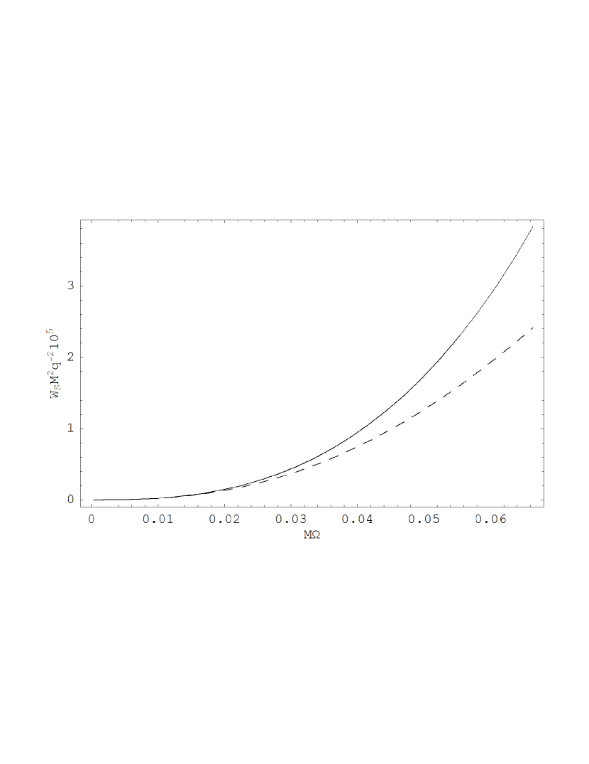
Figure 2: The total power $W_{S}$ emitted by the electric charge rotating around a Schwarzschild black hole is plotted as a function of the angular velocity $\Omega$ as measured by asymptotic static observers. The solid line represents our numerical result whereas the dashed line represents our analytic result for low frequencies. The $l$ summation in Eq. (45) is performed up to $l=6$. $M\Omega$ ranges from $0$ up to $0.068$ (associated with the innermost stable circular orbit at $R_{S}=6M$).

Let us now relate the radial coordinate $R_{S}$ of the rotating charge with its angular velocity $\Omega$. According to General Relativity for a stable circular orbit around a Schwarzschild black hole we have Wald

$$R_{S}=\left({M}/{\Omega^{2}}\right)^{1/3}\text{.}$$ (48)

We use this relation to compute numerically the emitted power given by Eqs. (45)-(47) as a function of $\Omega$. The numerical method used here is analogous to the one described in Ref. CHM2CQG . The result is plotted as the solid line in Fig. 2. The main contribution to the emitted power comes from modes with angular momentum $l=m=1$. The larger the $l$, the less is the contribution to the total radiated power. For a fixed value of $l$, the dominant contribution comes from $m=l$. Performing the summation up to $l=6$ in Eq. (45), modes with $l=m=1$ give almost all the contribution in the asymptotic region, while they contribute with about 65% at $R_{S}=6M$ (the innermost stable circular orbit according to General Relativity). In this case, the modes with $l=6$ contribute with less than 0.3% of the total radiated power for any position of the rotating charge.

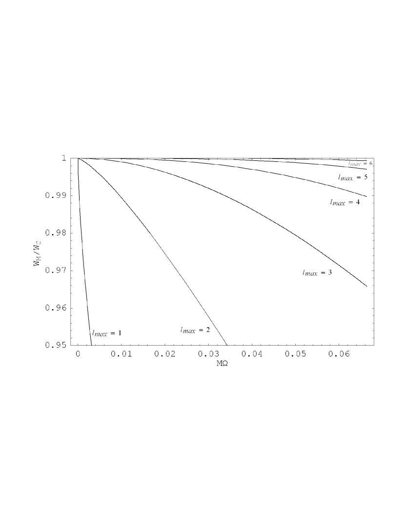
Figure 3: The ratio $W_{M}/W_{C}$ is plotted as a function of $\Omega$ considering an increasing number of contributions of the angular momentum $l$. We perform the summation from $l=1$ up to $l=l_{max}$ with $l_{max}$ varying from $1$ to $6$. We see that $W_{M}$ rapidly approaches the value of $W_{C}$ as we increase $l_{max}$. We also verify that it is important to consider large angular momentum contributions as the charge approaches the central object.

It is interesting to note that the magnitude of the total radiated power in the electromagnetic case is approximately twice the numerical result found previously for a scalar source coupled to a massless Klein-Gordon field CHM2CQG . In principle, this is not surprising because of the fact that photons have two physical polarizations. Notwithstanding, it should be emphasized that the two polarizations contribute quite differently to the emitted power. For our rotating charge, the contribution from mode $\lambda={\rm II}$ is negligible when compared with the one from mode $\lambda={\rm I}$ for every choice of $(n,\omega,l,m)$. Considering angular momentum contributions up to $l=6$, the ratio between the emitted power associated with modes $\lambda={\rm II}$ and $\lambda={\rm I}$ is always less than 0.1%.

Next, we use our low-frequency expressions for the physical modes, Eqs. (34)-(39), [and Eq. (48)] in Eqs. (45)-(47) to obtain an analytic approximation for the emitted power. The result is plotted as the dashed line in Fig. 2. We see from it that the numerical and analytical results differ sensibly as the charge approaches the black hole but coincide asymptotically, since far away from the hole only low frequency modes contribute to the emitted power.

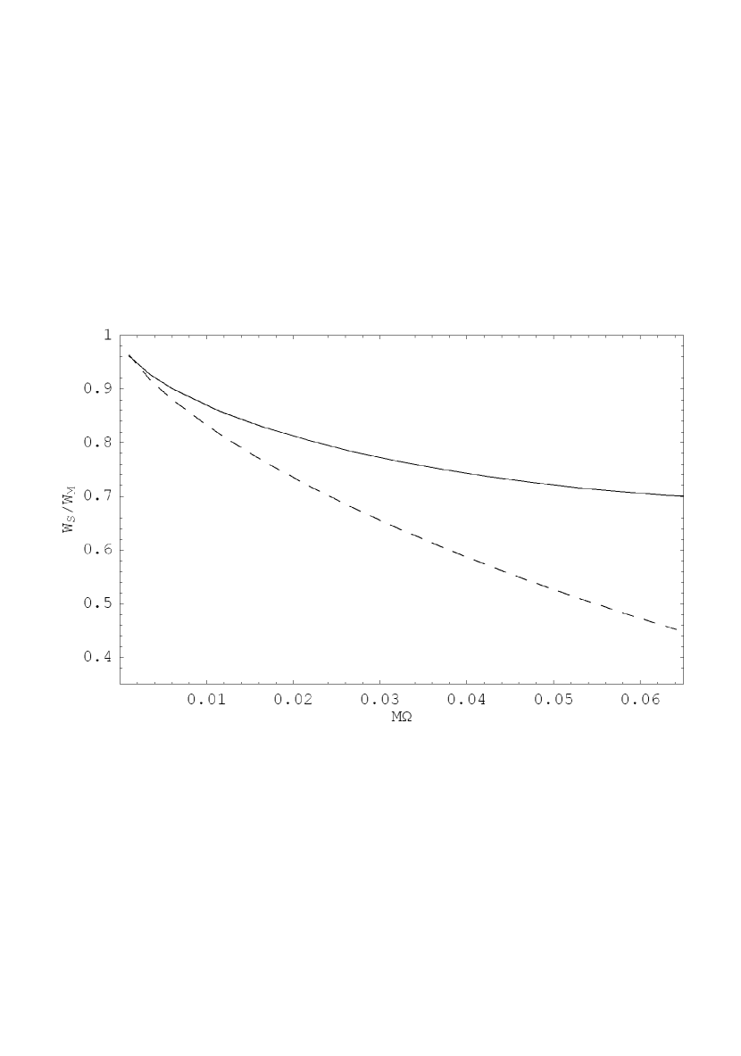
Figure 4: The ratio $W_{S}/W_{M}$ is plotted as a function of the angular velocity $\Omega$. Again we consider contributions of the angular momentum up to $l=6$ in the summations in Eqs. (45) and (50). The maximum value of $M\Omega$ is 0.068. The solid line corresponds to our numerical result, while the dashed line corresponds to our analytical low-frequency approximation result.

IV Comparison with flat spacetime results

In order to exhibit how better a full curved spacetime calculation can be in comparison with a flat spacetime one, let us show how the results found in the previous session differ from the ones obtained in Minkowski spacetime. In the latter case, the rotating charge is represented by the conserved current density

$$j_{M}^{\mu}\left(x^{\nu}\right) = \dfrac{q}{R_{M}^{2}}\delta\left(r-R_{M}\right)\delta\left(\theta-\pi/2\right)\delta\left(\phi-\Omega t\right)$$ (49)

$$\times \left(1,0,0,\Omega\right)\text{.}$$

This is formally identical to Eq. (40) but it is important to keep in mind that $R_{S}$ and $R_{M}$ are associated with Schwarzschild and Minkowski radial coordinates, respectively, which cannot be identified. The charge is regarded now as moving in a circular orbit due to a Newtonian gravitational force around a central object with the same mass $M$ as the black hole. In order to relate the radial coordinate $R_{M}$ with the angular velocity $\Omega$ (which is assumed to be measured by the same asymptotic static observers as before), we use the Keplerian relation: $R_{M}=M^{1/3}\Omega^{-2/3}$.

The quantization of the electromagnetic field can be performed analogously to the procedure exhibited in Section II by making $f=1$. As a consequence, the scattering potential $V_{S}$ in Eq. (12) is replaced by $V_{M}={l(l+1)}/{r^{2}}$. In Fig. 1 we plot the Minkowski scattering potential for $l=1$ (see dashed line).

Assuming the same minimal coupling between the charge and the electromagnetic field as before, we obtain that the emitted power at the tree level is given by

$$W_{M} = \frac{9q^{2}\Omega^{16/3}}{2}\sum_{l=1}^{\infty}\sum_{m=1}^{l}\dfrac{m^{2}}{l(l+1)}\left[\dfrac{d}{d\Omega}\left[\Omega^{-2/3}~{}j_{l}\left(m\left(\Omega M\right)^{1/3}\right)\right]\right]^{2}\left|Y_{lm}\left(\pi/2,0\right)\right|^{2}$$ (50)

$$+ 2q^{2}\Omega^{8/3}M^{2/3}\sum_{l=1}^{\infty}\sum_{m=1}^{l}m^{2}\left[j_{l}\left(m\left(\Omega M\right)^{1/3}\right)\right]^{2}\left|Y_{\phi}^{lm}\left(\pi/2,0\right)\right|^{2}\,.$$

The modes responsible for the dominant contributions to the radiated power follow the same pattern as in the Schwarzschild case. In particular, the contribution from the physical modes $\lambda={\rm II}$ is negligible when compared with the contribution from the physical modes $\lambda={\rm I}$.

As a consistency check for the flat spacetime results, we compare our quantum-oriented calculations with classical-oriented ones which lead to the Larmor formula for the total emitted power. Applying it to the case of a Keplerian circular orbit, we obtain

$$W_{C}=\dfrac{q^{2}M^{2/3}\Omega^{8/3}\gamma_{M}^{4}}{6\pi}$$ (51)

with $\gamma_{M}=(1-{M}^{2/3}\Omega^{2/3})^{-1/2}\text{.}$ In Fig. 3 we plot the ratios between $W_{M}$ and $W_{C}$, where the summations in Eq. (50) are performed up to increasing values of $l=l_{\rm max}$. We see that for $l_{max}=6$ the difference between $W_{M}$ and $W_{C}$ is less than 0.1% for $R_{M}>6M$. This is in agreement with the fact that the contributions associated with higher values of $l$ are negligible to the emitted power.

Next we compare our curved and flat spacetime results using our previous expressions for $W_{S}$ and $W_{M}$ as functions of the physical observables $M$ and $\Omega$ as measured by asymptotic static observers. We plot the ratio between $W_{S}$ and $W_{M}$ in Fig. 4 obtained from our numerical computations (solid line) and from our low-frequency analytic approximation (dashed line). In both cases the ratio tends to the unity as the charge rotates far away from the attractive center, as a consequence of the fact that the Schwarzschild spacetime is asymptotically flat. As the rotating charge approaches the central object, curved and flat spacetime results differ more significantly. In the innermost relativistic stable circular orbit, the numerical computation gives that $W_{S}$ is 30% smaller than $W_{M}$. We emphasize that this is not a simple consequence of the red-shift effect, since the mode functions representing the quanta of the emitted radiation are quite different in curved and flat spacetimes.

V Absorption of the electromagnetic radiation by the black hole

Now, this is interesting to use our quantum field theory in Schwarzschild spacetime approach to compute what is the amount of emitted radiation which can be asymptotically observed. This is given by

$$W_{S}^{obs}=\sum_{\lambda={\rm I},{\rm II}}\sum_{l=1}^{\infty}\sum_{m=1}^{l}\left[|T_{\omega_{0}l}^{\lambda\rightarrow}|^{2}W_{S}^{\lambda\rightarrow\omega_{0}lm}\right.$$

$$\left.+|R_{\omega_{0}l}^{\lambda\leftarrow}|^{2}W_{S}^{\lambda\leftarrow\omega_{0}lm}\right]\,.$$ (52)

Our numerical result is shown as the solid line in Fig. 5. In order to compute $W_{S}^{obs}$ in the low-frequency approximation (see dashed line in Fig. 5) we calculate the expressions for the transmission and reflection coefficients. For this purpose we use

$$Q_{l}\approx\dfrac{2^{l}\left(l!\right)^{2}}{\left(2l+1\right)!}z^{-l-1}\,\,\,\,\,\left(z\gg 1\right)$$ (53)

in Eq. (34) to write

$$r{\varphi}_{\omega l}^{\lambda\rightarrow}\approx C_{\omega l}^{\lambda\rightarrow}\,\dfrac{2^{l}\left(l+1\right)\left(l!\right)^{2}M^{l+1}}{l\left(2l+1\right)!}\,x^{-l}\,\,\,\,\,\left(x\gg 1\right)\,\,\text{.}$$ (54)

Comparing the above expression with Eq. (29) and using that $h_{l}^{\left(1\right)}\left(x\right)\approx\eta_{l}\left(x\right)\approx\dfrac{-\left(2l\right)!}{2^{l}l!}x^{-l-1}$ for $x\gg 1$, we obtain

$$|T_{\omega l}^{\lambda\rightarrow}|=\dfrac{|C_{\omega l}^{\lambda\rightarrow}|}{|B_{\omega l}^{\lambda\rightarrow}|}\,\dfrac{2^{2l}\left(l+1\right)\left(l!\right)^{3}M^{l+1}\omega^{l}}{l\left(2l\right)!\left(2l+1\right)!}$$ (55)

with the normalization constants given by Eqs. (31), (32), (36) and (37). The reflexion coefficients are determined using that $\left|R_{\omega l}^{\lambda\leftarrow}\right|^{2}=\left|R_{\omega l}^{\lambda\rightarrow}\right|^{2}=1-\left|T_{\omega l}^{\lambda\rightarrow}\right|^{2}$.

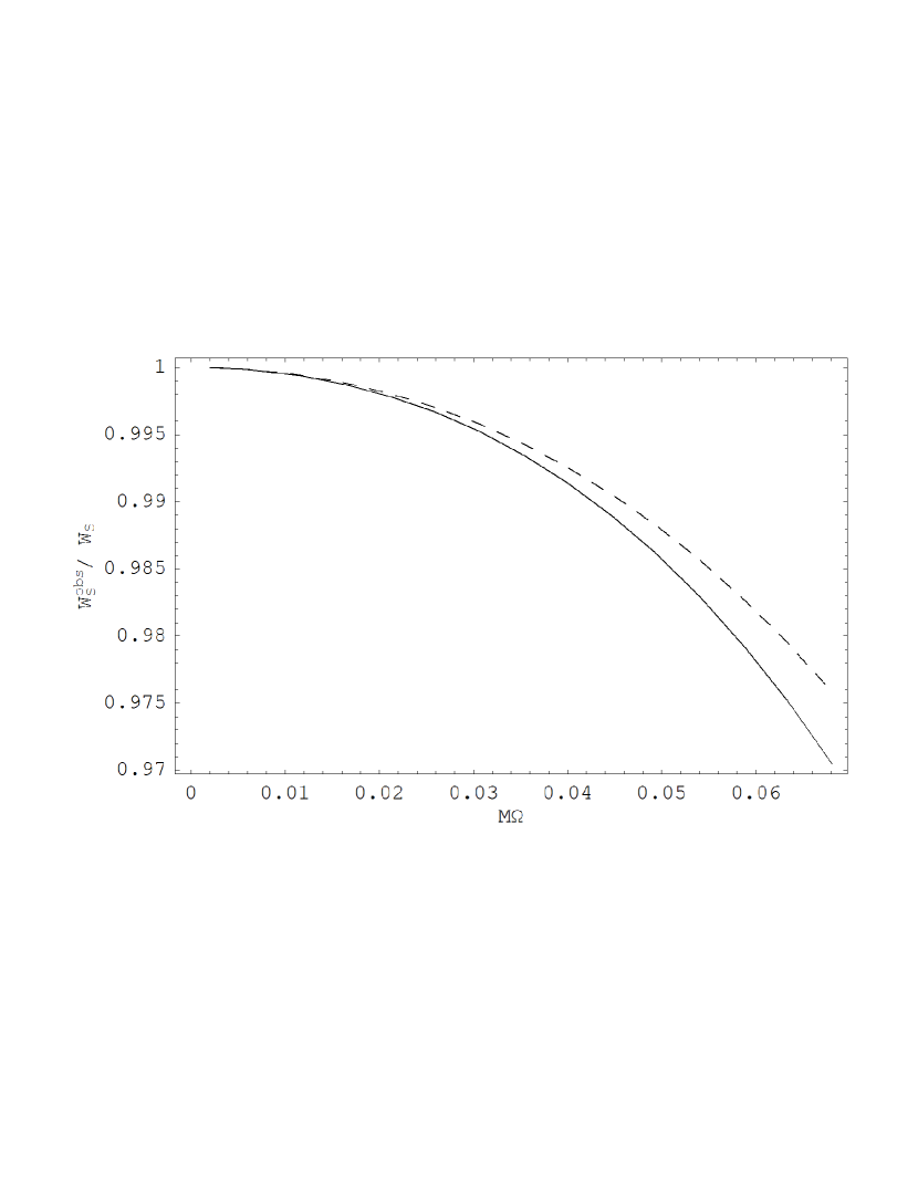
Figure 5: The ratio between the asymptotically observed power $W_{S}^{obs}$ and the emitted power $W_{S}$ is plotted as a function of the angular velocity $\Omega$ of the swirling electric charge according to asymptotic static observers. $M\Omega$ varies from 0 to $0.068$. The summations in Eqs. (52) and (45) are performed up to $l=6$.

We see from Fig. 5 that the black hole absorbs only a small amount of the emitted radiation. Even for the innermost stable circular orbit the black hole absorbs only $3\%$ of the total radiated power. These results are consistent with the fact that the absorption cross section of a Schwarzschild black hole is proportional to $\omega^{2}$ for small frequency photons (see, e.g., Page ).

VI Final Remarks

In this paper we have considered the radiation emitted by an electric charge rotating around a chargeless static black hole in the context of quantum field theory in curved spacetimes. We have obtained that the two physical photon polarizations give very different contributions to the total emitted power. Indeed, the contribution of one of the physical modes is negligible as compared with the other one. As a consistency check of our procedure we have computed, using a similar approach, the emitted power from a charge in Minkowski spacetime rotating around a massive object due to a Newtonian force and showed that this is in agreement with Larmor’s classical result. Then we compared the radiation emitted (as measured by asymptotic static observers) considering the attractive central object with mass $M$ as (i) a Schwarzschild black hole and (ii) a Newtonian massive object in flat spacetime. We have obtained that curved and flat spacetime results coincide when the charge orbits far away from the massive object but differ considerably when the charge orbits close to it. The difference reaches 30% for the innermost stable circular orbit. This result corroborates the importance of considering the curvature of the spacetime in astrophysical phenomena occurring in the vicinity of black holes when they involve particles with wavelengths of the order of the event horizon radius. Finally, we have computed the amount of the emitted radiation which is absorbed by the black hole. We have shown that most of the emitted radiation can be asymptotically observed. For the case of the innermost stable circular orbit at $R_{S}=6M$, about 97% of the emitted power can be in principle detected at infinity.

- (1) J. van Paradijs and J. E. McClintock, in X–Ray Binaries, eds. W. H. G. Lewin, J. van Paradijs and E. P. J. van den Heuvel (Cambridge University Press, Cambridge, 1995).
- (2) M. J. Rees, in Black holes and relativistic stars, ed. R. M. Wald (The University of Chicago Press, Chicago, 1998).
- (3) R. Genzel et al, Nature 425, 934 (2003); B. C. Bromley, W. A. Miller and V. I. Pariev, Nature 391, 54 (1998); Y. Tanaka et al, Nature 375, 659 (1995); R. Narayan, I. Yi and R. Mahadevan, Nature 374, 623 (1995); M. J. Rees et al, Nature 295, 17 (1982).
- (4) L. C. B. Crispino, A. Higuchi and G. E. A. Matsas, Class. Quant. Grav. 17, 19 (2000).
- (5) N. D. Birrell and P. C. W. Davies, Quantum fields in curved space (Cambridge University Press, Cambridge, 1982).
- (6) B. P. Jensen and P. Candelas, Phys. Rev. D 33, 1590 (1986); 35, 4041(E) (1987).
- (7) I. S. Gradshteyn and I. M. Ryzhik, Tables of Integrals, Series, and Products (Academic Press, New York, 1980).
- (8) L. C. B. Crispino, A. Higuchi and G. E. A. Matsas, Phys. Rev. D 63, 124008 (2001).
- (9) A. Higuchi, Class. Quant. Grav. 4, 721 (1987).
- (10) L. C. B. Crispino, A. Higuchi and G. E. A. Matsas, Phys. Rev. D 58, 084027 (1998).
- (11) C. Itzykson and J. -B. Zuber, Quantum Field Theory (McGraw-Hill, New York, 1980).
- (12) D. G. Boulware, Phys. Rev. D 11, 1404 (1975); 12, 350 (1975).
- (13) M. Abramowitz and I. A. Stegun, Handbook of Mathematical Functions (Dover Publications, New York, 1965).
- (14) R. M. Wald, General Relativity (The University of Chicago Press, Chicago, 1984).
- (15) D. N. Page, Phys. Rev. D 13, 198 (1976).