Dimensional regularization of the third post-Newtonian gravitational wave generation from two point masses

Abstract

Dimensional regularization is applied to the computation of the gravitational wave field generated by compact binaries at the third post-Newtonian (3PN) approximation. We generalize the wave generation formalism from isolated post-Newtonian matter systems to $d$ spatial dimensions, and apply it to point masses (without spins), modelled by delta-function singularities. We find that the quadrupole moment of point-particle binaries in harmonic coordinates contains a pole when $\varepsilon\equiv d-3\rightarrow 0$ at the 3PN order. It is proved that the pole can be renormalized away by means of the same shifts of the particle world-lines as in our recent derivation of the 3PN equations of motion. The resulting renormalized (finite when $\varepsilon\rightarrow 0$) quadrupole moment leads to unique values for the ambiguity parameters $\xi$, $\kappa$ and $\zeta$, which were introduced in previous computations using Hadamard’s regularization. Several checks of these values are presented. These results complete the derivation of the gravitational waves emitted by inspiralling compact binaries up to the 3.5PN level of accuracy which is needed for detection and analysis of the signals in the gravitational-wave antennas LIGO/VIRGO and LISA.

I Introduction

A compelling motivation for accurate computations of the gravitational radiation field generated by compact binary systems (i.e., made of neutron stars and/or black holes) is the need for accurate templates to be used in the data analysis of the current and future generations of laser interferometric gravitational wave detectors. It is indeed recognized that the inspiral phase of the coalescence of two compact objects represents an extremely important source for the ground-based detectors LIGO/VIRGO, provided that their total mass does not exceed say 10 or 20 $M_{\odot}$ (this includes the interesting case of double neutron-star systems), and for space-based detectors like LISA, in the case of the coalescence of two galactic black holes, if the masses are within the range between say $10^{5}$ and $10^{8}\,M_{\odot}$.

For these sources the post-Newtonian (PN) approximation scheme has proved to be the appropriate theoretical tool in order to construct the necessary templates. A program started long ago with the goal of obtaining these templates with 3PN and even 3.5PN accuracy. Several studies Cutler et al. (1993); Cutler and Flanagan (1994); Tagoshi and Nakamura (1994); Poisson (1995); Damour et al. (1998, 2000a); Buonanno et al. (2003); Damour et al. (2003); Ajith et al. (2005); Arun et al. (2005) have shown that such a high PN precision is probably sufficient, not only for detecting the signals in LIGO/VIRGO, but also for analyzing them and accurately measuring the parameters of the binary (such high-accuracy templates will also be of great value for detecting massive black-hole mergers in LISA). The templates have been first completed through 2.5PN order, for both the phase Blanchet et al. (1995a, b); Will and Wiseman (1996); Blanchet (1996) and wave amplitude Blanchet et al. (1996); Arun et al. (2004). The 3.5PN accuracy for the templates (in the case where the compact objects have negligible intrinsic spins) has been achieved more recently, in essentially two steps.

1. The first step has been to compute all the terms, in both the 3PN equations of motion, either in Hamiltonian form Jaranowski and Schäfer (1998, 1999); Damour et al. (2000b, 2001a) or using harmonic coordinates Blanchet and Faye (2000a, 2001); de Andrade et al. (2001); Blanchet and Iyer (2003), and the 3.5PN gravitational radiation field, using a multipolar wave generation formalism Blanchet (1998a); Blanchet et al. (2002a, b); Blanchet and Iyer (2004), by means of the Hadamard self-field regularization Hadamard (1932); Schwartz (1978); Sellier (1994); Blanchet and Faye (2000b), in short HR. (The 3.5PN terms in the equations of motion have been added in Refs. Pati and Will (2000); Königsdörffer et al. (2003); Nissanke and Blanchet (2005).) However, a few terms were left undetermined by Hadamard’s regularization, which corresponds to some incompleteness of this regularization occurring at the 3PN order. These terms could be parametrized by some unknown numerical coefficients called ambiguity parameters.

2. The second step has been to fix the values of the ambiguity parameters by means of dimensional regularization ’t Hooft and Veltman (1972); Bollini and Giambiagi (1972); Breitenlohner and Maison (1977), henceforth abbreviated as DR. Technically, DR is based on analytic continuation in the dimension of space $d=3+\varepsilon$. The ambiguity parameter $\lambda$ entering the 3PN equations of motion has been computed in Refs. Damour et al. (2001b); Blanchet et al. (2004a), with result $\lambda=-1987/3080$. (This result has also been obtained with an alternative approach in Refs. Itoh et al. (2001); Itoh and Futamase (2003); Itoh (2004).) The three ambiguity parameters appearing in the 3PN gravitational radiation field will be shown in the present paper to have the following unique values

   $$\xi=-\frac{9871}{9240}\,,\qquad\kappa=0\,,\qquad\zeta=-\frac{7}{33}\,,$$ (1)

   as already announced in Ref. Blanchet et al. (2004b). The method we use for applying DR essentially consists in computing the difference between DR and some appropriately defined Hadamard-type regularization called below the pure-Hadamard-Schwartz (pHS) regularization.

Those results complete the determination of the 3.5PN-accurate phase evolution as it suffices to insert into the formulas of Ref. Blanchet et al. (2002b) the value for $\lambda$, together with the values given by (1). Actually, this phase evolution depends only on $\lambda$ and on the following particular combination of parameters,

$$\theta\equiv\xi+2\kappa+\zeta=-\frac{11831}{9240}\,.$$ (2)

The present paper is devoted to the details of our DR computation of the ambiguity parameters, item (2) above, which has led to the values (1)–(2). We refer to Blanchet et al. (2004b) for a summary of our method and a general discussion.

Let us emphasize that the values (1), which constitute the end result of the application of DR, have all been confirmed by alternative methods. Our first independent check has been the confirmation of one particular combination of the ambiguity parameters, namely $\xi+\kappa$, which was shown to follow from the requirement that the 3PN mass dipole moment of the binary, computed in Blanchet and Iyer (2004) from the multipolar wave generation formalism, should agree with the 3PN center-of-mass position, known from the conservative part of the 3PN equations of motion in harmonic coordinates de Andrade et al. (2001). Secondly, we have also obtained the value of $\zeta$ by considering the limiting physical situation of a boosted Schwarzschild solution, corresponding to the case where the mass of one of the particles is exactly zero, and the other particle moves with uniform velocity Blanchet et al. (2005). It can be argued from this calculation that the value of $\zeta$ in Eq. (1) is a consequence of the global Poincaré invariance of the multipolar wave generation formalism. Thirdly, in Sec. VII below, we shall be able to show that the value of $\kappa$ is zero by a diagrammatic approach (where the “diagrams” are taken in the sense of Damour and Esposito-Farèse (1996)), showing that no dangerously divergent diagrams contributing to $\kappa$ appear at this order. Those checks altogether provide a confirmation, independent from DR, for all the parameters (1).

The plan of this paper is as follows. In Section II we investigate the symmetric-trace-free (STF) multipole decomposition in $d$ dimensions for a scalar field with compact-support source. In Section III we generalize to $d$ dimensions the known results for the multipole expansion of the gravitational field and the definition of the source-type multipole moments. Section IV is devoted to the explicit expressions of the source terms in the latter source multipole moments at the 3PN order in terms of a convenient set of retarded-like elementary potentials. Then, in Section V, we obtain a general formula for the difference between DR and HR (in the pHS variant of it). This difference is non-zero at the 3PN order because of the occurrence of poles in $d$ dimensions (i.e., $\propto 1/\varepsilon$). In Section VI we deduce the ambiguity parameters from the DR regularization of the 3PN mass quadrupole moment, and we check that the 3PN mass dipole is in agreement with the known center-of-mass position deduced from the equations of motion. Section VII deals with a direct computation of the pole part of the moments using diagrams, their renormalization using shifts of the world-lines, and the check that $\kappa=0$. In Section VIII we present an alternative derivation of the value of $\zeta$ based on considering the physical situation of a single boosted point particle in $d$ dimensions (the result agrees with the recent computation of the boosted Schwarzschild solution in Blanchet et al. (2005)).

II Multipole expansion of a scalar field in $d$ dimensions

A crucial input for the derivations we are going to perform in the present article is the multipolar expansion of solutions of flat space-time wave equations in $D=d+1$ dimensions. We denote by $\Box=\eta^{\mu\nu}\partial_{\mu}\partial_{\nu}$ the flat d’Alembertian operator, using the signature “mostly plus”, i.e., $\Box=\Delta-c^{-2}\partial^{2}_{t}$, where $\partial_{t}\equiv\partial/\partial t$ and $\Delta$ is the Laplace operator. We first consider the case of a scalar wave equation, say

$$\Box\varphi(\mathbf{x},t)=S(\mathbf{x},t)\,,$$ (3)

and shall postpone to Sec. III the case of tensorial wave equations. Note that, in the present work, we shall not introduce any numerical factor in the “source” $S$ on the right hand side (RHS) of the inhomogeneous scalar wave equation (3). Similarly, we define the scalar Green functions as the solutions of

$$\Box G(\mathbf{x},t)=\delta(t)\,\delta^{(d)}(\mathbf{x})\,,$$ (4)

where $\delta^{(d)}(\mathbf{x})$ is a $d$-dimensional Dirac distribution, such that $\int d^{d}\mathbf{x}\,\delta^{(d)}(\mathbf{x})\,f(\mathbf{x})=f(\mathbf{0})$. When $d=3$, the retarded Green function takes the simple form

$$G^{(3+1)}_{\mathrm{Ret}}(\mathbf{x},t)=-\frac{\delta\left(t-|\mathbf{x}|/c\right)}{4\pi\,|\mathbf{x}|}\,.$$ (5)

Because of the presence of the factor $-1/4\pi$ in (5), it was convenient, when working in $3+1$ dimensions, to introduce a factor $-4\pi$ in front of the RHS’s of (3) and (4). However, there is no analogous, universally simplifying factor in $D$ dimensions, so it is finally simpler to introduce no factors at all in (3)–(4).

The $D$-dimensional retarded Green function has no simple expression in $(t,\mathbf{x})$ space. However, starting from its well-known Fourier-space expression, one can write the following simple integral expression (see e.g. Cardoso et al. (2003)),

$$G_{\mathrm{Ret}}(\mathbf{x},t)=-\frac{\theta(t)}{(2\pi)^{d/2}}\int_{0}^{+\infty}dk\left(\frac{k}{r}\right)^{\frac{d}{2}-1}\sin(c\,k\,t)\,J_{\frac{d}{2}-1}(k\,r)\,.$$ (6)

Notice that this is in fact a function of $t$ and $r\equiv|\mathbf{x}|$ only: say $G_{\mathrm{Ret}}(\mathbf{x},t)=G_{\mathrm{Ret}}(r,t)$. Here $\theta(t)$ is the Heaviside step function, and $J_{\frac{d}{2}-1}(k\,r)$ the usual Bessel function. Actually, we shall never need to use the explicit form (6) of the Green function in $D$ dimensions. Indeed, we shall obtain the $d$-dimensional generalizations of the $3$-dimensional relativistic multipole moments, obtained in Refs. Blanchet (1995, 1998b); Poujade and Blanchet (2002), by working directly with the source $S$ of the wave equation (3), or of its tensor generalizations. To do this, we note first that the retarded solution of (3) reads

$$\varphi(\mathbf{x},t)=\int d^{d}\mathbf{y}\,ds\,G_{\mathrm{Ret}}(\mathbf{x}-\mathbf{y},t-s)\,S(\mathbf{y},s)\,.$$ (7)

In this section, we shall consider sources $S(\mathbf{x},t)$ having a spatially compact support in $d$ space dimensions: say $S(\mathbf{x},t)=0$ when $|\mathbf{x}|>a$, where $a$ is the source’s radius. We are interested in the multipolar expansion of the field $\varphi(\mathbf{x},t)$, i.e., its decomposition (when considered in the external domain $|\mathbf{x}|>a$) in $d$-dimensional spherical harmonics. Traditionally, the multipolar expansion of $\varphi(\mathbf{x},t)$, Eq. (7), is obtained by expanding the spatial kernel $G_{\mathrm{Ret}}(\mathbf{x}-\mathbf{y})$ in powers of $|\mathbf{y}|\rightarrow 0$. This introduces the (reducible) multipole moments of the source, say $\int d^{d}\mathbf{y}\,y^{i_{1}}\cdots y^{i_{\ell}}\,S(\mathbf{y})$. A simpler, formally equivalent way of proceeding is to replace the continuous source $S(\mathbf{x})$ by its “distributional skeleton”, i.e., an expansion in increasing derivatives of the $d$-dimensional Dirac distribution $\delta(\mathbf{x})$. [For notational simplicity, we henceforth suppress the superscript $(d)$ on $\delta(\mathbf{x})$.] This skeletonized version of the source $S$ is equivalent to a continuous function $S(\mathbf{x})$ with compact support when (and only when) it is integrated by a regular kernel $K(\mathbf{x},\mathbf{y})$, as in (7). It reads

$$S^{\mathrm{Skel}}(\mathbf{x},t)=\sum_{\ell=0}^{+\infty}\frac{(-)^{\ell}}{\ell!}\,S_{L}(t)\,\partial_{L}\delta(\mathbf{x})\,,$$ (8)

where the coefficients are the reducible multipole moments

$$S_{L}(t)=\int d^{d}\mathbf{y}\,y_{L}\,S(\mathbf{y},t)\,.$$ (9)

We recall our simplified notation: $L$ denotes a multi-index $i_{1}\cdots i_{\ell}$ and we use the shorthands $\partial_{L}\equiv\partial_{i_{1}}\cdots\partial_{i_{\ell}}$, where $\partial_{i}\equiv\partial/\partial x^{i}$, and $y_{L}\equiv y_{i_{1}}\cdots y_{i_{\ell}}$, where $y_{i}\equiv y^{i}$.

The skeleton expansion (8) does not yet give rise to a multipole expansion because the various terms on the RHS of (8) do not correspond to irreducible representations of the $d$-dimensional rotation group $O(d)$. However, it is relatively simple to transform the expansion (8) into irreducible components. To do this, it is enough to decompose the symmetric tensors $S_{L}$ into irreducible symmetric and trace-free (STF) pieces, which is easily done by using the STF decomposition of $y_{L}$ in $d$ dimensions, obtained by recursively separating the traces, like in $y_{ij}\equiv\widehat{y}_{ij}+\frac{1}{d}\,\delta_{ij}\,|\mathbf{y}|^{2}$. Here we denote the STF projection by means of a hat: $\widehat{y}_{L}\equiv\mathrm{STF}[y_{i_{1}}\cdots y_{i_{\ell}}]$, or sometimes by means of brackets surrounding the indices: $\widehat{y}_{L}\equiv y_{\langle L\rangle}$. The general formula defined by this recursion has already been given in Ref. Blanchet et al. (2004a) and reads

$$y_{L} = \sum_{k=0}^{[\frac{\ell}{2}]}\,a_{\ell}^{k}\,\delta_{\{i_{1}i_{2}}\cdots\delta_{i_{2k-1}i_{2k}}\,\widehat{y}_{L-2K\}}\,|\mathbf{y}|^{2k},$$ (10a)

$$\text{with}\quad a_{\ell}^{k} \equiv \frac{1}{2^{k}}\frac{\Gamma\left(\frac{d}{2}+\ell-2k\right)}{\Gamma\left(\frac{d}{2}+\ell-k\right)}\,.$$ (10b)

Here, $\delta_{ij}$ is the Kronecker symbol, $[\frac{\ell}{2}]$ denotes the integer part of $\frac{\ell}{2}$, $L-2K$ is a multi-index with $\ell-2k$ indices, and $\Gamma$ is the usual Eulerian function. The curly brackets surrounding the indices refer to the (unnormalized, minimal) sum of the permutations of the indices which keep the object fully symmetric in $L$, for instance $\delta_{\{ij}V_{k\}}\equiv\delta_{ij}V_{k}+\delta_{ik}V_{j}+\delta_{jk}V_{i}$ (for convenience we do not normalize the latter sum).

We replace the STF decomposition (10) into (9) and insert the resulting moments back into Eq. (8). After some simple manipulations we arrive at

$$S^{\mathrm{Skel}}(\mathbf{x},t) = \sum_{\ell=0}^{+\infty}\frac{(-)^{\ell}}{\ell!}\sum_{k=0}^{+\infty}\alpha_{\ell}^{k}\,\Delta^{k}\partial_{L}\left[\delta(\mathbf{x})\int d^{d}\mathbf{y}\,\widehat{y}_{L}\,|\mathbf{y}|^{2k}\,S(\mathbf{y},t)\right],$$ (11a)

$$\text{where}\quad\alpha_{\ell}^{k} \equiv \frac{1}{2^{2k}k!}\frac{\Gamma\left(\frac{d}{2}+\ell\right)}{\Gamma\left(\frac{d}{2}+\ell+k\right)}\,.$$ (11b)

At this point let us notice that any term in the skeletonized source $S^{\mathrm{Skel}}(\mathbf{x},t)$ which is in the form of a d’Alembert operator $\Box$ acting on spatial gradients or time derivatives of the delta function, say $\Box\left[\partial\,\delta(\mathbf{x})\right]$, will give no contribution to the multipole expansion of $\varphi(\mathbf{x},t)$. Indeed, a term in the source of the form $\Box^{i+1}\left[f(t)\,\partial_{L}\delta(\mathbf{x})\right]$, with $i\geq 0$, $\ell\geq 0$, will yield a contribution to the solution of the form $\Box^{-1}_{\mathrm{Ret}}\left(\Box^{i+1}\left[f(t)\,\partial_{L}\delta(\mathbf{x})\right]\right)=\Box^{i}\left[f(t)\,\partial_{L}\delta(\mathbf{x})\right]$. Such a contribution is localized at the spatial origin $\mathbf{x}=\mathbf{0}$ and thus vanishes outside of the world tube $r\leq a$ containing the source.

We now transform the Laplacians in (11) into d’Alembertians using

$$\Delta^{k}=\left(\Box+\frac{1}{c^{2}}\partial_{t}^{2}\right)^{k}=\sum_{j=0}^{k}\frac{k!}{j!(k-j)!}\,\Box^{j}\left(\frac{1}{c^{2}}\partial_{t}^{2}\right)^{k-j}.$$ (12)

We then arrive at an irreducible (STF) decomposition of the skeletonized source $S$, which is of the type

$$S^{\mathrm{Skel}}(\mathbf{x},t)=\sum_{\ell=0}^{+\infty}\frac{(-)^{\ell}}{\ell!}\,\widehat{S}_{L}(t)\,\partial_{L}\delta(\mathbf{x})+\mathcal{O}\left(\Box\,\partial\,\delta\right).$$ (13)

Here the last term, symbolically denoted $\mathcal{O}\left(\Box\,\partial\,\delta\right)$, is an (infinite) sum of terms of the form $\Box^{i+1}[f(t)\partial_{L}\delta(\mathbf{x})]$ with $i\geq 0$, $\ell\geq 0$. As we just said, these terms will not contribute to the multipole expansion of the field $\varphi(\mathbf{x},t)$, i.e., considered in the external domain $r>a$.

The most useful result for our purpose is the explicit expression of the STF moments in Eq. (13) which we find to be

$$\widehat{S}_{L}(t)=\int d^{d}\mathbf{y}\,\widehat{y}_{L}\,\overline{S}_{\ell}(\mathbf{y},t)\,,$$ (14)

where we have introduced a convenient $\ell$-dependent weighted time average given by the formal infinite PN series

$$\overline{S}_{\ell}(\mathbf{y},t)=\sum_{k=0}^{+\infty}\alpha_{\ell}^{k}\left(\frac{|\mathbf{y}|}{c}\frac{\partial}{\partial t}\right)^{2k}S(\mathbf{y},t)\,.$$ (15)

The coefficients $\alpha_{\ell}^{k}$ are those which have been introduced in Eq. (11b). When written out explicitly, the “effective” source $\overline{S}_{\ell}(\mathbf{y},t)$ reads,

$$\overline{S}_{\ell}(\mathbf{y},t) = S(\mathbf{y},t)+\frac{1}{2(2\ell+d)}\left(\frac{|\mathbf{y}|}{c}\frac{\partial}{\partial t}\right)^{2}S(\mathbf{y},t)+\cdots$$

$$+ \frac{1}{(2k)!!(2\ell+d)(2\ell+d+2)\cdots(2\ell+d+2k-2)}\left(\frac{|\mathbf{y}|}{c}\frac{\partial}{\partial t}\right)^{2k}S(\mathbf{y},t)+\cdots\,,$$

where $(2k)!!\equiv(2k)(2k-2)\cdots(2)$.

Note that the result (14)–(II) for the scalar relativistic multipoles in $d$ dimensions is a remarkably simple generalization of the $3$-dimensional result obtained in Blanchet and Damour (1989): It is enough to replace the explicit $3$’s, $5$’s etc. appearing in Eq. (B.14b) of Blanchet and Damour (1989) by $d$, $d+2$, etc., without changing anything else. In Blanchet and Damour (1989) it was also shown that the expansion (II) was in $3$ dimensions the PN expansion of the exact result

$$\overline{S}_{\ell}^{\,(d=3)}(\mathbf{y},t) = \int_{-1}^{1}dz\,\delta_{\ell}^{(0)}(z)\,S(\mathbf{y},t+z|\mathbf{y}|/c)\,,$$ (17a)

$$\text{with}\qquad\delta_{\ell}^{(0)}(z) \equiv \frac{\Gamma\left(\ell+\frac{3}{2}\right)}{\Gamma\left(\frac{1}{2}\right)\Gamma\left(\ell+1\right)}\,(1-z^{2})^{\ell}\,,\qquad\int_{-1}^{1}dz\,\delta_{\ell}^{(0)}(z)=1\,.$$ (17b)

The ratio of Gamma functions appearing in Eq. (17b) is equal to $(2\ell+1)!!/(2^{\ell+1}\ell!)$. Note that since the expansion is purely “even” (i.e., with only even powers of $c^{-1}$), the time argument $t+z|\mathbf{y}|/c$ in (17a) can be equivalently changed into $t-z|\mathbf{y}|/c$.

Correspondingly, one can check that the $d$-dimensional result (15)–(II) is the PN expansion of the following simple generalization of the $3$-dimensional case:

$$\overline{S}_{\ell}^{(\varepsilon)}(\mathbf{y},t)=\int_{-1}^{1}dz\,\delta_{\ell}^{(\varepsilon)}(z)\,S(\mathbf{y},t+z|\mathbf{y}|/c)\,,$$ (18)

where we introduced $\varepsilon\equiv d-3$, and

$$\delta_{\ell}^{(\varepsilon)}(z)\equiv\frac{\Gamma\left(\ell+\frac{3}{2}+\frac{\varepsilon}{2}\right)}{\Gamma\left(\frac{1}{2}\right)\Gamma\left(\ell+1+\frac{\varepsilon}{2}\right)}\,(1-z^{2})^{\ell+\frac{\varepsilon}{2}},\qquad\int_{-1}^{1}dz\,\delta_{\ell}^{(\varepsilon)}(z)=1\,.$$ (19)

Consistently with what happened in Eq. (II), the kernel $\delta_{\ell}^{(\varepsilon)}(z)$ is simply obtained from its $3$-dimensional limit by replacing everywhere $\ell$ by $\ell+\frac{\varepsilon}{2}$ (i.e., $2\ell$ by $2\ell+d-3$):

$$\delta_{\ell}^{(\varepsilon)}(z)=\delta_{\ell+\frac{\varepsilon}{2}}^{(0)}(z)\,.$$ (20)

Let us mention in passing that the “exact” re-summed expression (18) can also be directly derived from the Fourier-space expression of the $d$-dimensional Green’s function.

Finally, having obtained the STF decomposition of the source term $S^{\mathrm{Skel}}$ in the form (13), we obtain the corresponding expression of the scalar field $\varphi(\mathbf{x},t)$. As we pointed out above, the remainder term in Eq. (13) does not contribute to the multipolar expansion of the field. Henceforth we shall denote by $\mathcal{M}(\varphi)$ the multipolar expansion of $\varphi$, which is therefore given by

$$\mathcal{M}(\varphi)(\mathbf{x},t)=\sum_{\ell=0}^{+\infty}\frac{(-)^{\ell}}{\ell!}\,\Box_{\mathrm{Ret}}^{-1}\left(\widehat{S}_{L}(t)\,\partial_{L}\delta(\mathbf{x})\right),$$ (21)

since the terms $\Box_{\mathrm{Ret}}^{-1}\mathcal{O}\left(\Box\,\partial\,\delta\right)$ give zero when considered outside the compact support of the source. In terms of the retarded Green’s function the latter formula becomes

$$\mathcal{M}(\varphi)(\mathbf{x},t)=\sum_{\ell=0}^{+\infty}\frac{(-)^{\ell}}{\ell!}\,\partial_{L}\left[\int_{-\infty}^{+\infty}ds\,\widehat{S}_{L}(s)\,G_{\mathrm{Ret}}(\mathbf{x},t-s)\right].$$ (22)

Note that, in view of the retarded nature of the Green function $G_{\mathrm{Ret}}(\mathbf{x},t-s)$, the integral is limited to $s<t$, and even to $s<t-r/c$ with $r\equiv|\mathbf{x}|$. Equation (22) generalizes what was the basic result for the multipolar expansion of a $3$-dimensional inhomogeneous wave equation $\Box^{\,(d=3)}\varphi=S$, namely

$$\mathcal{M}(\varphi)^{\,(d=3)}(\mathbf{x},t)=-\frac{1}{4\pi}\sum_{\ell=0}^{+\infty}\frac{(-)^{\ell}}{\ell!}\,\partial_{L}\left(\frac{\widehat{S}_{L}^{\,(d=3)}(t-r/c)}{r}\right).$$ (23)

A common feature of the result (23) and its $d$-dimensional generalization (22) is that each “multipolar wave” of degree $\ell$ is obtained by an $\ell$-tuple differentiation, with respect to the spatial coordinates, of an elementary spherically symmetric (i.e., monopolar) retarded solution; indeed, as mentioned above $G_{\mathrm{Ret}}(\mathbf{x},t-s)$ depends only on $r$ and $t-s$. In $3$ dimensions the elementary spherically symmetric retarded solutions admit a simple expression in terms of the multipole moments, namely $\widehat{S}_{L}^{\,(d=3)}(t-r/c)/r$. By contrast, the $d$-dimensional analogue of each elementary spherically symmetric solution is a more complicated non-local functional of $\widehat{S}_{L}(s)$, which involves an integral over its time argument: $\int_{-\infty}^{t-r/c}ds\,\widehat{S}_{L}(s)\,G_{\mathrm{Ret}}(r,t-s)$. This non-locality in time in the expression of $\varphi$ in terms of $\widehat{S}_{L}$ comes in addition to the non-locality in time entering the exact definition (18) of the effective source term $\overline{S}_{\ell}^{(\varepsilon)}(\mathbf{y},t)$. The former non-locality is evidently related to the fact that the “Huygens principle” holds only in $d=3$, $5$, $7$, $\cdots$ dimensions. In these special dimensions, the support of the retarded Green function $G_{\mathrm{Ret}}(r,t-s)$ is concentrated on the past light cone $s=t-r/c$. On the other hand, in other dimensions (and notably in dimensionally-continued complex ones) the support of the retarded Green function $G_{\mathrm{Ret}}(r,t-s)$ extends over the interior of the past light cone: $s\leq t-r/c$.

III Multipole decomposition of the gravitational field

III.1 $d$-dimensional generalization of the multipolar post-Minkowskian formalism

The calculations of the 3.5PN templates, Refs. Blanchet (1998a); Blanchet et al. (2002a, b); Blanchet and Iyer (2004), applied the general expressions of the relativistic multipole moments of Refs. Blanchet (1995, 1998b); Poujade and Blanchet (2002), which are themselves to be inserted into the (3-dimensional) multipolar post-Minkowskian (MPM) formalism of Ref. Blanchet and Damour (1986). Let us sketch how one can, in principle, generalize this MPM formalism to arbitrary dimensions $d$. The basic building blocks of the MPM formalism are:

1. the parametrization of a general solution of the linearized vacuum Einstein equations in harmonic coordinates, say $h^{\mu\nu}$, by means of several sequences of irreducible multipole moments;

2. the definition of an integral operator, called $\mathop{\mathrm{FP}}\Box^{-1}_{\mathrm{Ret}}$, which produces, when it is applied to the non-linear effective MPM source $N_{n}^{\mu\nu}=N_{n}^{\mu\nu}(h_{1},h_{2},\ldots,h_{n-1})$ appearing at the $n^{\text{th}}$ non-linear iteration, a particular non-linear solution, $p_{n}^{\mu\nu}$, of the inhomogeneous wave equation $\Box p_{n}^{\mu\nu}=N_{n}^{\mu\nu}$;

3. the definition of a complementary homogeneous solution $q_{n}^{\mu\nu}$ ($\Box q_{n}^{\mu\nu}=0$) such that $h_{n}^{\mu\nu}\equiv p_{n}^{\mu\nu}+q_{n}^{\mu\nu}$ satisfies the harmonicity condition $\partial_{\nu}h_{n}^{\mu\nu}=0$.

Given these building blocks, the MPM formalism generates, by iteration, a general solution of the non-linear vacuum Einstein equations as a formal power series, $\sqrt{-g}g^{\mu\nu}=\eta^{\mu\nu}+Gh_{1}^{\mu\nu}+\cdots+G^{n}h_{n}^{\mu\nu}+\cdots$, this solution being parametrized by the arbitrary “seed” multipole moments entering the definition of the first approximation $h_{1}^{\mu\nu}$. We briefly indicate how the various building blocks can be generalized to arbitrary dimensions $d$. We have in mind here an extension to generic integer dimensions $d>3$, before defining a formal continuation to complex dimensions. [We consider mainly larger dimensions $d>3$ because they exhibit generic $d$-dependent features, while lower integer dimensions, $d=1,2$, exhibit special phenomena.]

In the previous section we have discussed the multipole expansion of scalar fields, $\Box\varphi=S$, in arbitrary $d$. We have seen that the general (retarded) solution outside the source $S$ could be parametrized, in any $d$, by a set of symmetric trace-free (STF) time-dependent tensors $\widehat{S}_{L}(t)$. The situation is somewhat more complicated for other fields, notably the spin-2 field $h^{\mu\nu}$ relevant for gravity in any $d$. As we shall discuss in the next subsection, the multipole moments needed in a generic $d>3$ to parametrize a general gravitational field are more complicated than what can be used in $d=3$. In $d=3$, one can use two independent sets of STF tensors, say $M_{L}$ (the “mass multipole moments”) and $S_{L}$ (the “spin multipole moments”). In a generic $d>3$, one has still the analogue of the mass multipole moments, i.e., STF tensors $M_{L}$ corresponding to a Young tableau made of $\ell$ horizontal boxes (). However, the spin multipole moments must be described by a mixed Young tableau having one vertical column of two boxes and $\ell-1$ complementary horizontal ones — so that there are $\ell$ boxes on the upper horizontal row (). In addition, one must introduce a third type of irreducible representation of the $d$-dimensional rotation group $O(d)$, namely a mixed Young tableau having two vertical columns of two boxes and $\ell-2$ complementary horizontal ones (). For instance, when $\ell=2$, this new irreducible representation has the symmetry of a Weyl tensor in $d$ dimensions: . As is well known, this representation does not occur in $d\leq 3$. However, all these technical complications will have little impact on what we will need to calculate here. Indeed, as discussed below, it will be enough for our purpose of unambiguously computing the 3PN-level gravitational radiation emission to deal with the simpler mass multipole moments $M_{L}$, which admit a uniform treatment in any dimension $d$ (actually we shall use a specific definition for what we call the source-type mass multipole moments and denote them by $I_{L}$ instead of $M_{L}$).

Let us turn to the generalization of the integral operator $\mathop{\mathrm{FP}}\Box^{-1}_{\mathrm{Ret}}$. In $d=3$, the precise definition of this operator was the following. Consider a typical non-linear source generated by the MPM iteration, e.g. $N_{2}=N_{2}(h_{1},h_{1})\sim(\partial h_{1})^{2}+h_{1}\partial^{2}h_{1}$, in which $h_{1}$ is represented by its multipole expansion. One formally assumes that the multipole expansion of $h_{1}\sim\sum\partial\left[M_{L}(t-r/c)/r\right]$ contains a finite number of multipoles. This ensures that the non-linear source $N_{2}(h_{1})$ is a finite sum of terms of the form $\widehat{n}_{K}F(t-r/c)/r^{q}$, with angular factor $\widehat{n}_{K}=\mathrm{STF}\left(n^{i_{1}}\cdots n^{i_{k}}\right)$, $n^{i}=x^{i}/r$. We can further expand $F(t-r/c)$ in powers of $r/c$ and get $N_{2}(h_{1})$ as a sum of terms $\sim\widehat{n}_{K}F(t)/r^{p}$. Though this multipole expansion of $N_{2}(h_{1})$ is only physically relevant in the region outside the source, say $r>a$, in the MPM formalism we always mathematically extend its definition (by real, analytic continuation in $r$) down to $r=0$. Then this formal construction, $h_{\mathrm{MPM}}=G\,h_{1}+G^{2}\,h_{2}+\cdots$, valid by real analytic continuation for any $r>0$, is identified with the multipolar expansion, say $\mathcal{M}(h)$, of the physical field $h$. While the physical $h$ takes different expressions inside ($r<a$) and outside ($r>a$) the source, the object $\mathcal{M}(h)\equiv h_{\mathrm{MPM}}$ is mathematically defined everywhere (except at $r=0$) by the same formal expression, but is physically correct only when $r>a$ (see Blanchet (1998b) for the notation and further discussion).

To deal with the singular behavior near $r=0$ of the non-linear MPM source terms, e.g. $N_{2}(h_{1})\sim\widehat{n}_{K}F(t)/r^{p}$, one introduces a complex number $B$ and considers the action of the retarded Green operator onto the product of the source by a “regularization” factor $(r/r_{0})^{B}$, say

$$F_{2}^{(d=3)}(B)\equiv\Box_{\mathrm{Ret}}^{-1}\left[\left(\frac{r}{r_{0}}\right)^{B}N_{2}(h_{1})\right].$$ (24)

The length scale $r_{0}$ represents an arbitrary dimensionful parameter serving the purpose of adimensionalizing the above regularization factor. It was shown in Ref. Blanchet and Damour (1986) that the integral $F_{2}(B)$, Eq. (24), is convergent when the real part of $B$ is large enough, and that $F_{2}(B)$, considered as a function of the complex number $B$, is a meromorphic function of $B$, which has in general (simple) poles at $B=0$, coming from the singular behavior of the integrand $N_{2}(h_{1})$ near $r=0$. [One formally assumes that the multipole moments are time-independent before some instant $-\mathcal{T}$, and at the end of the calculation the limit $\mathcal{T}\rightarrow+\infty$ is taken.] Therefore, the Laurent expansion of $F_{2}(B)$, near $B=0$, is of the form

$$F_{2}^{(d=3)}(B)=\frac{C_{-1}(\mathbf{x},t)}{B}+C_{0}(\mathbf{x},t)+C_{1}(\mathbf{x},t)B+\mathcal{O}\left(B^{2}\right).$$ (25)

One then defines, when $d=3$, the finite part at $B=0$ of $\Box^{-1}_{\mathrm{Ret}}N_{2}(h_{1})$, denoted $\mathrm{FP}\,\Box^{-1}_{\mathrm{Ret}}N_{2}(h_{1})$, as the term $C_{0}(\mathbf{x},t)$ in the Laurent expansion of $F_{2}(B)$. One proves that $C_{0}(\mathbf{x},t)$ satisfies the equation $\Box C_{0}=N_{2}(h_{1})$ and uses it as the “particular” second-order contribution $p_{2}^{\mu\nu}$ to the second-order metric $h_{2}^{\mu\nu}$. Let us not spend time on the construction of the additional homogeneous contribution $q_{2}^{\mu\nu}$ necessary to satisfy the harmonicity condition $\partial_{\nu}\left(p_{2}^{\mu\nu}+q_{2}^{\mu\nu}\right)=0$ [an example of construction of such contribution will be given in (64) below]. Having so constructed (in $d=3$) the second-order term in the MPM expansion of the external metric, $h_{2}^{\mu\nu}=p_{2}^{\mu\nu}+q_{2}^{\mu\nu}$, one continues the iteration by considering the next order inhomogeneous equation $\Box h_{3}=N_{3}\left(h_{1},h_{2}\right)$ and introducing $F_{3}(B)\equiv\Box_{\mathrm{Ret}}^{-1}\left[(r/r_{0})^{B}N_{3}(h_{1},h_{2})\right]$. The singular behavior near $r=0$ of $N_{3}$ is more complicated (it contains logarithms of $r$), and, as a consequence, one finds that $F_{3}(B)$ is still meromorphic in the complex $B$ plane, but will contain double poles at $B=0$. Again, one defines $p_{3}=\mathop{\mathrm{FP}}\Box^{-1}_{\mathrm{Ret}}N_{3}$ as the coefficient of the zero-th power of $B$ in the Laurent expansion of $F_{3}(B)$ when $B\rightarrow 0$.

Having recalled the definition and properties of the operation $\mathop{\mathrm{FP}}\Box^{-1}_{\mathrm{Ret}}$ in the 3-dimensional MPM formalism, let us sketch what changes when working in $d$ dimensions. Let us start with the “seed” linearized metric $h_{1}^{\mu\nu}$. As we see in Eq. (21), and will see below with more details for the tensorial analogue of the scalar multipole expansion, the multipole expansion $h_{1}$ is of the form $h_{1}\sim\sum\partial\,\Box_{\mathrm{Ret}}^{-1}\left[M_{L}(t)\delta(\mathbf{x})\right]$. Though one cannot write, in arbitrary $d$, a simple, closed-form expression for the object $\Box_{\mathrm{Ret}}^{-1}\left[M_{L}(t)\delta(\mathbf{x})\right]$, it is enough to write down its expansion when $r\rightarrow 0$ (which is in fact the same as its PN expansion). Modulo regular terms near the origin, this expansion is obtained as

$$\Box_{\mathrm{Ret}}^{-1}\Bigl{[}M_{L}(t)\delta(\mathbf{x})\Bigr{]} = \left(\Delta^{-1}+\frac{1}{c^{2}}\,\partial_{t}^{2}\Delta^{-2}+\frac{1}{c^{4}}\,\partial_{t}^{4}\Delta^{-3}+\cdots\right)\Bigl{[}M_{L}(t)\delta(\mathbf{x})\Bigr{]}$$ (26)

$$+~{}\text{regular terms}.$$

Using $\Delta^{-1}\delta(\mathbf{x})\propto r^{2-d}$, $\Delta^{-2}\delta(\mathbf{x})\propto r^{4-d}$ etc. we see that the 3-dimensional form of the expansion of $h_{1}$ near $r=0$ (after taking into account the expansion of the retardation $r/c$), takes in $d$ dimensions the form

$$h_{1}\sim\sum\frac{\widehat{n}_{K}F(t)}{r^{p+\varepsilon}}\,,$$ (27)

where $\widehat{n}_{K}\equiv\mathrm{STF}[n_{i_{1}}\cdots n_{i_{k}}]$, $p$ is a (relative) integer, and $\varepsilon\equiv d-3$. Inserting this expansion in the second-order source $N_{2}(h_{1})\sim\partial h_{1}\partial h_{1}+h_{1}\partial^{2}h_{1}$ yields

$$N_{2}\left(h_{1}\right)\sim\sum\frac{\widehat{n}_{K}F(t)}{r^{p+2\varepsilon}}\,.$$ (28)

At this stage, one could consider $\Box_{\mathrm{Ret}}^{-1}N_{2}$, without inserting a factor $(r/r_{0})^{B}$, by using the analytic continuation in $d$. However, to ensure continuity with what was done in $3$ dimensions, it is better to insert this factor and to consider

$$F_{2}^{(d)}(B)\equiv\Box_{\mathrm{Ret}}^{-1}\left[\left(\frac{r}{r_{0}}\right)^{B}N_{2}\left(h_{1}\right)\right].$$ (29)

The main difference between (29) and its 3-dimensional analogue (24) concerns the meromorphic structure of $F_{2}(B)$. Indeed, in view of the shift by $+2\varepsilon$ of the integer exponent $p$ in (28), and of the presence of $r^{\varepsilon}$ in the $d$-dimensional volume element $d^{d}\mathbf{x}=r^{2+\varepsilon}dr\,d\Omega_{2+\varepsilon}$, one easily sees that the (simple) poles in $F_{2}(B)$ that were located at $B=0$ when $d=3$ are no longer located at $B=0$ when $d\neq 3$, but are shifted at $B=2\varepsilon-\varepsilon=\varepsilon$. Alternatively, this can be explicitly verified by using the expansion $\Box^{-1}_{\mathrm{Ret}}=\Delta^{-1}+c^{-2}\partial_{t}^{2}\Delta^{-2}+\cdots$ (plus a regular kernel), and the formula $\Delta^{-1}r^{\alpha}=r^{\alpha+2}/[(\alpha+2)(\alpha+d)]$ where the pole at $\alpha=-d$ is the only one which comes from the ultraviolet (UV) behavior $r\rightarrow 0$. As a consequence, the expansion (25) is now modified to

$$F_{2}^{(d)}(B)=\frac{C_{-1}^{(d)}(\mathbf{x},t)}{B-\varepsilon}+C_{0}^{(d)}(\mathbf{x},t)+C_{1}^{(d)}(\mathbf{x},t)B+\mathcal{O}\left(B^{2}\right).$$ (30)

This expansion, and its analogues considered below, is considered for $\varepsilon$ and $B$ both small (so that the expansion in powers of $B$ makes sense), but without assuming any relative ordering between the smallness of $B$ and that of $\varepsilon$. One should neither re-expand $(B-\varepsilon)^{-1}$ in powers of $B/\varepsilon$ nor in powers of $\varepsilon/B$.

Having in hand the above structure, one then defines the $d$-dimensional generalization of the finite part of $N_{2}(h_{1})$ as the coefficient of $B^{0}$ in Eq. (30), namely $C_{0}^{(d)}$. We denote such a finite part by

$$\mathop{\mathrm{FP}}_{B}\Box^{-1}_{\mathrm{Ret}}\Bigl{[}\widetilde{r}^{B}N_{2}\left(h_{1}\right)\Bigr{]} \equiv C_{0}^{(d)}(\mathbf{x},t)\,,$$ (31a)

$$\text{where}~{}~{}\widetilde{r} \equiv \frac{r}{r_{0}}\,,$$ (31b)

or, more simply, by

$$\mathrm{FP}\,\Box^{-1}_{\mathrm{Ret}}N_{2}\left(h_{1}\right)\equiv\mathrm{FP}\,F_{2}^{(d)}\equiv C_{0}^{(d)}(\mathbf{x},t)\,.$$ (32)

Note the subtlety that the expansion (30) is neither a Laurent expansion in powers of $B-\varepsilon$, nor a Laurent expansion in powers of $B$. After subtracting the shifted pole terms $\propto(B-\varepsilon)^{-1}$, one expands the remainder in a regular Taylor series in powers of $B$. The interest of this specific definition is the fact that it ensures that $C_{0}^{(d)}(\mathbf{x},t)$ is an exact solution of the equation we initially wanted to solve, namely

$$\Box^{(d)}C_{0}^{(d)}=N_{2}\left(h_{1}\right).$$ (33)

Indeed, by its mere definition (29), one has $\Box F_{2}^{(d)}(B)=(r/r_{0})^{B}N_{2}(h_{1})$. Comparing this result (which has no pole) to the application of $\Box$ to (30), we first see that the pole part must be a homogeneous solution, $\Box C_{-1}^{(d)}=0$. Then, identifying the successive powers of $B$ (using ${\widetilde{r}}^{B}=e^{B\ln\widetilde{r}}=1+B\ln\widetilde{r}+\cdots$), yields $\Box C_{0}^{(d)}=N_{2}$, $\Box C_{1}^{(d)}=\ln(r/r_{0})N_{2}$, and so on. Another useful property of the $d$-modified definition (31) is that it automatically ensures the continuity between $d\rightarrow 3$ and $d=3$. Indeed, the shift in the location of the pole in (30) was made to “follow” the pole that existed at $B=0$ when $d=3$. Therefore we have $\lim_{d\rightarrow 3}C_{-1}^{(d)}=C_{-1}$, and similarly $\lim_{d\rightarrow 3}C_{0}^{(d)}=C_{0}$, etc., where the RHSs are those defined in Eq. (25) when $d=3$.

The extension of the iteration to higher non-linear orders introduces a new subtlety. Indeed, let us look more precisely at the structure of the second-order contribution to the metric, $h_{2}=p_{2}+q_{2}$ where, as we said, the particular solution $p_{2}$ is defined by the modified FP process: $p_{2}\equiv\mathrm{FP}\,\Box^{-1}_{\mathrm{Ret}}N_{2}(h_{1})$, and where $q_{2}$ is a complementary homogeneous solution. Most of the terms in the integrand $N_{2}$ introduce no poles, and, for them, we simply find a structure of the type $p_{2}^{\mathrm{(no\,pole)}}\sim\sum r^{-p-2\varepsilon}$ (for simplicity, we henceforth suppress angular factors). Let us now consider the terms in $N_{2}$ that generate poles $\propto(B-\varepsilon)^{-1}$ in $F_{2}(B)$. We know that such terms introduce, when $d=3$, some logarithms of the radial variable $r$. When $d\neq 3$, they no longer introduce logarithms but they introduce a further technical complication. Indeed, let us look at a typical example, namely a dangerous term in $F_{2}(B)$ of the form $F_{2}^{\mathrm{(pole)}}(B)=\Delta^{-1}(r^{B-3-2\varepsilon})$. Suppressing for simplicity a factor $(B-1-2\varepsilon)^{-1}$ which is jointly analytic in $B$ and $\varepsilon$ near $B=0$ and $\varepsilon=0$ respectively and therefore creates no problem, we have essentially $F_{2}^{\mathrm{(pole)}}(B)=(B-\varepsilon)^{-1}r^{B-1-2\varepsilon}$. According to Eq. (30) the pole part of $F_{2}^{\mathrm{(pole)}}$ that we must subtract is, for instance, obtained by multiplying by $B-\varepsilon$ and then taking the limit $B\rightarrow\varepsilon$ (and not $B\rightarrow 0$). This pole part is therefore given by $(B-\varepsilon)^{-1}r^{-1-\varepsilon}$. The finite part of $F_{2}^{\mathrm{(pole)}}(B)$ is then obtained by subtracting the pole part and taking the limit $B\rightarrow 0$; this yields

$$p_{2}^{\mathrm{(pole)}}=\mathrm{FP}\,F_{2}^{\mathrm{(pole)}}=\frac{1}{\varepsilon}\left[r^{-1-\varepsilon}-r^{-1-2\varepsilon}\right].$$ (34)

The subtlety is that there seems to appear poles in $\varepsilon^{-1}$. However, the residue of the pole vanishes, since the limit $\varepsilon\rightarrow 0$ of (34) is finite and generates the logarithm that we know to exist in $d=3$, $p_{2}^{\mathrm{(pole)}}\sim\ln r/r$. If we do not take the limit $\varepsilon\rightarrow 0$, we must keep the structure (34) and see what it generates at the next, cubic, order of iteration. In addition, we must also add the complementary solution $q_{2}$ needed to satisfy the harmonicity condition, $\partial_{\nu}(p_{2}^{\mu\nu}+q_{2}^{\mu\nu})=0$. As the calculation of $q_{2}$ could be done in $d=3$ without encountering poles (see Ref. Blanchet and Damour (1986)), it will clearly not create problems in $d\neq 3$ apart from the fact that $q_{2}$, being a homogeneous solution $\Box q_{2}=0$, will behave near $r=0$ essentially like $h_{1}$, i.e., $q_{2}\sim\sum r^{-p-\varepsilon}$ (which differs from most of the terms of $p_{2}$ which were $\sum r^{-p-2\varepsilon}$).

Summarizing so far, the second-order MPM iteration $h_{2}$ has a structure, near $r=0$, of the symbolic form

$$h_{2}\sim\sum c_{1}(\varepsilon)\,r^{-p-\varepsilon}+c_{2}(\varepsilon)\,r^{-p-2\varepsilon}+\frac{c_{3}(\varepsilon)}{\varepsilon}\left[r^{-p-\varepsilon}-r^{-p-2\varepsilon}\right],$$ (35)

where the $c_{i}(\varepsilon)$’s are analytic at $\varepsilon=0$, and where we explicitly separated the semi-singular structure in $\varepsilon$. When inserting the structure (35) into $N_{3}(h_{1},h_{2})$, one finds that the singular behavior of $N_{3}$ near $r=0$ can generate several types of singularities in $B$ and $\varepsilon$. There are simple poles $\propto(B-\varepsilon)^{-1}$ and simple poles $\propto(B-2\varepsilon)^{-1}$, which are natural generalizations of the structures that generated simple poles in $F_{2}(B)$. When looking at the effect of the more complicated structure given by the third term on the RHS of (35), one finds that it is best described as generating some “quasi-double poles”, namely terms $\propto(B-\varepsilon)^{-1}(B-2\varepsilon)^{-1}$. The point is that if one were to expand this term in simple poles with respect to $B$, namely

$$\frac{1}{(B-\varepsilon)(B-2\varepsilon)}=\frac{1}{\varepsilon(B-2\varepsilon)}-\frac{1}{\varepsilon(B-\varepsilon)}\,,$$ (36)

it would seem to involve poles in $1/\varepsilon$. However, all such poles are “spurious” because the source of the trouble which is the last term in (35) had a finite limit as $\varepsilon\rightarrow 0$, and because one can easily see that, in our above-defined MPM algorithm, source terms having a finite limit as $\varepsilon\rightarrow 0$ generate solutions having also a finite limit as $\varepsilon\rightarrow 0$.

Finally we find, by induction, that at each iteration order $n$ one has the structure

$$h_{n}\sim\sum d_{1}(\varepsilon)\,r^{-p-\varepsilon}+d_{2}(\varepsilon)\,r^{-p-2\varepsilon}+\cdots+d_{n}(\varepsilon)\,r^{-p-n\varepsilon}\,,$$ (37)

where the coefficients $d_{i}(\varepsilon)$ might individually have (simple or multiple) poles in $\varepsilon$, e.g. $d_{i}(\varepsilon)=c_{i}(\varepsilon)/\varepsilon^{j}$, but which always compensate each other in the complete sum $h_{n}$. Then we obtain that the integral

$$F_{n}^{(d)}(B)\equiv\Box_{\mathrm{Ret}}^{-1}\Bigl{[}\widetilde{r}^{B}N_{n}\left(h_{1},\cdots,h_{n-1}\right)\Bigr{]}$$ (38)

will have an expansion, near $B=0$, of the generic form

$$F_{n}^{(d)}(B)=\sum\frac{C_{-k}^{(d)}(\mathbf{x},t)}{(B-q_{1}\varepsilon)(B-q_{2}\varepsilon)\cdots(B-q_{k}\varepsilon)}+C_{0}^{(d)}(\mathbf{x},t)+C_{1}^{(d)}(\mathbf{x},t)B+\mathcal{O}\left(B^{2}\right).$$ (39)

The “quasi-multiple poles” which constitute the first term on the RHS have $k\leq n-1$ and $1\leq q_{i}\leq n-1$. As we have seen in (35) and (37), the poles in $1/\varepsilon$ are in fact spurious, as they have a residue which is always zero. [We assume here that the seed multipole moments are regular as $\varepsilon\rightarrow 0$.] So, when writing the result in the form of (39), we note that the coefficients $C_{-k}^{(d)}$, $C_{0}^{(d)}$, etc., are all regular when $d\rightarrow 3$. One then defines the $d$-dimensional generalization of the finite part of $F_{n}^{(d)}$ as being the coefficient of $B^{0}$ in the expansion (39):

$$p_{n}=\mathrm{FP}\,F_{n}^{(d)}\equiv C_{0}^{(d)}(\mathbf{x},t)\,.$$ (40)

This coefficient is regular when $\varepsilon\equiv d-3\rightarrow 0$, though it contains apparently singular terms of the type of the last term on the RHS of (35). Moreover, using the same reasoning as above, one finds that it satisfies the needed result: $\Box p_{n}=N_{n}$. Note finally that, when $\varepsilon\rightarrow 0$, the quasi-multiple poles in (39) merge together to form the multiple poles $\propto B^{-k}$, with $k\leq n-1$, that were found to exist in $d=3$ Blanchet and Damour (1986). On the other hand, when $\varepsilon\neq 0$, the poles form a “line” of simple poles located at $B=\varepsilon$, $B=2\varepsilon$, $\cdots$, $B=(n-1)\varepsilon$. However, it is better not to decompose the product of simple poles entering (39) in sum of separate simple poles, because this decomposition would, as in Eq. (36), introduce spurious singularities $\propto\varepsilon^{-j}$.

The main practical outcome of the present subsection is the modified definition of the operation $\mathrm{FP}\,\Box^{-1}_{\mathrm{Ret}}$ when working in $d\neq 3$: namely as the coefficient of $B^{0}$ in an expansion of the type (39) where, after separating the shifted poles at $B-\varepsilon$, $\cdots$, $B-(n-1)\varepsilon$, one expands the remainder in a Taylor series in powers of $B$. Note that a simple consequence of this definition is that, for instance, a term of the form $B/(B-q\varepsilon)$ in $\Box^{-1}_{\mathrm{Ret}}\left[\widetilde{r}^{B}N_{n}\right]$ gives rise to a finite part equal to 1. Indeed,

$$\mathrm{FP}\left[\frac{B}{B-q\varepsilon}\right]=\mathrm{FP}\left[\frac{B-q\varepsilon+q\varepsilon}{B-q\varepsilon}\right]=\mathrm{FP}\left[\frac{q\varepsilon}{B-q\varepsilon}+1\right]=1\,.$$ (41)

One might have been afraid that a term of this type, $B/(B-q\varepsilon)$, could have been ambiguous because, ultimately, we are sending both $B$ and $\varepsilon$ towards zero without fixing an ordering between the two limits. However, in the present $d$-dimensional generalization of the MPM formalism, everything is precisely defined and unambiguous.

III.2 Multipolar decomposition of the gravitational field in $d$ dimensions

We now sketch the $d$-dimensional generalization of the results concerning the matching between the MPM exterior metric and the inner field of a general post-Newtonian (PN) matter system. To start with, we consider the case of a smooth matter distribution, and will later allow the matter stress-energy tensor to tend to a distribution localized on some world-lines. The next subsection will be devoted to the $d$-dimensional definition of the source multipole moments. The investigations of this and the next subsection are based on the works Blanchet (1995, 1998b); Poujade and Blanchet (2002) which derived the expressions of the source multipole moments of a general PN source, up to any PN order (in $3$ dimensions). Early derivations of the relativistic moments, valid up to 1PN order, can be found in Refs. Blanchet and Damour (1989); Damour and Iyer (1991a).

We look for a solution, in the form of a PN expansion, of the $d$-dimensional Einstein field equations. As before we choose some harmonic coordinates, which means that $\partial_{\nu}h^{\mu\nu}=0$ where the so-called “gothic” metric deviation reads $h^{\mu\nu}\equiv\sqrt{-g}\,g^{\mu\nu}-\eta^{\mu\nu}$, where $g$ is the determinant and $g^{\mu\nu}$ the inverse of the usual covariant metric $g_{\rho\sigma}$. Then the Einstein field equations, relaxed by the harmonic coordinate conditions, take the form of some “scalar” wave equations, similar to (3), for each of the components of $h^{\mu\nu}$,

$$\Box h^{\mu\nu}=\frac{16\pi\,G}{c^{4}}\,\tau^{\mu\nu}\,,$$ (42)

where $\Box$ denotes the $d$-dimensional flat space-time wave operator, and $G$ is the $d$-dimensional Newton constant related to the usual Newton constant $G_{N}$ in $3$ dimensions by Eq. (81) below. The main contribution we shall add in the present subsection, with respect to our investigation of the scalar wave equation in Sec. II, is how to deal with the crucial non-linear gravitational source term in the Einstein field equations, which makes the RHS of Eq. (42) to have a support which is spatially non-compact. The RHS of (42) involves what can be called the total stress-energy pseudo tensor of the non-gravitational and gravitational fields, given by

$$\tau^{\mu\nu}=|g|T^{\mu\nu}+\frac{c^{4}}{16\pi G}\Lambda^{\mu\nu}\bigl{(}h,\partial h,\partial^{2}h\bigr{)},$$ (43)

where $T^{\mu\nu}$ is the matter stress-energy tensor, and the second term represents the gravitational stress-energy distribution, which can be expanded into non-linearities according to

$$\Lambda^{\mu\nu}=\Lambda_{2}^{\mu\nu}(h,h)+\Lambda_{3}^{\mu\nu}(h,h,h)+\cdots\,,$$ (44)

where the quadratic, cubic, etc., pieces admit symbolic structures such as $\Lambda_{2}\sim h\,\partial^{2}h+\partial h\,\partial h$ and $\Lambda_{3}\sim h\,\partial h\,\partial h$.

The solution $h^{\mu\nu}$ of the field equations we consider in this subsection will be smooth and valid everywhere, inside as well as outside the matter source localized in the domain $r\leq a$. Inside the source, or more generally inside the source’s near zone ($r\ll\lambda$, where $\lambda$ is the wavelength of the emitted radiation), $h^{\mu\nu}$ will admit a PN expansion, denoted here as $\overline{h}^{\mu\nu}$. On the other hand, in the exterior of the source, $r>a$, $h^{\mu\nu}$ will admit a multipolar expansion, solution of the vacuum field equations outside the source, and decomposed into ($d$-dimensional) irreducible spherical harmonics. As usual, the definition of the multipole expansion is extended by real analytic continuation in $r$ to any value $r>0$. It will be necessary to introduce the special notation $\mathcal{M}(h^{\mu\nu})$ to mean the multipole expansion of $h^{\mu\nu}$. As we already mentioned, the multipole expansion in the present formalism is given by the MPM metric of Sec. III.1, which is therefore in the form of a formal infinite post-Minkowskian series up to any order $n$,

$$\mathcal{M}(h^{\mu\nu})\equiv h_{\mathrm{MPM}}^{\mu\nu}\,.$$ (45)

As mentioned above, though the identification (45) is only physically meaningful in the exterior domain $r>a$, it can be mathematically extended down to any $r>0$ by real analytic continuation in $r$.

In this subsection we shall show how to relate in $d$ dimensions the multipolar expansion (45) to the properties of the matter source, in the case of a PN source (i.e., one which is located deep inside its own near zone, $a\ll\lambda$). Actually, the derivation below will be a simple $d$-dimensional adaptation of the proof given in the case of $3$ dimensions in Ref. Blanchet (1998b) (see notably the Appendix A there).

The heart of the method is to show that one can deal with the presence of non-compact-support source terms on the RHS of the field equation (42), by considering a certain quantity $\Delta^{\mu\nu}$ which satisfies a wave equation whose source does have a compact support, and thus, whose multipolar expansion can be computed by using the results of Sec. II (for each space-time component $\mu\nu$). This quantity is defined by

$$\Delta^{\mu\nu}\equiv h^{\mu\nu}-\mathop{\mathrm{FP}}_{B}\,\Box^{-1}_{\mathrm{Ret}}\Bigl{[}\widetilde{r}^{B}\mathcal{M}(\Lambda^{\mu\nu})\Bigr{]}.$$ (46)

The second term in (46), that we thus subtract from $h^{\mu\nu}$ in order to define this quantity, involves the finite part operation FP in $d$-dimensions which has been defined in the previous subsection (III.1). It contains the regularization factor $\widetilde{r}^{B}\equiv(r/r_{0})^{B}$. The use of the operator $\mathrm{FP}\,\Box^{-1}_{\mathrm{Ret}}$ is consistent with Sec. III.1 because it acts on the multipole expansion of the non-linear source term $\mathcal{M}(\Lambda^{\mu\nu})$, which is in fact identical to the formal post-Minkowskian (MPM) infinite series $\Lambda_{\mathrm{MPM}}^{\mu\nu}$, cf. Eq. (45). The meaning of the last term on the RHS of (46) is that $\mathrm{FP}\,\Box^{-1}_{\mathrm{Ret}}$ is to be applied to each term of the MPM expansion of $\widetilde{r}^{B}\mathcal{M}(\Lambda^{\mu\nu})$, and that we then consider the formal summation of this MPM series.

Equation (46) appears to be the difference between the solution of the field equation (42) and the contribution coming only from the non-linear terms in the exterior of the compact-support source (and then analytically continued down to $r=0$). Since $h^{\mu\nu}$ is the retarded integral of the pseudo tensor $\tau^{\mu\nu}$, and since the multipole expansion of the matter tensor is formally zero: $\mathcal{M}(T^{\mu\nu})=0$ (because $T^{\mu\nu}$ has a compact support), we can rewrite (46) as

$$\Delta^{\mu\nu}=\frac{16\pi\,G}{c^{4}}\biggl{\{}\Box^{-1}_{\mathrm{Ret}}\tau^{\mu\nu}-\mathop{\mathrm{FP}}_{B}\,\Box^{-1}_{\mathrm{Ret}}\Bigl{[}\widetilde{r}^{B}\mathcal{M}(\tau^{\mu\nu})\Bigr{]}\biggr{\}}.$$ (47)

Next, we remark that the first term in (47) is regular within the source (for $r\leq a$), and that we can therefore add to it the same FP procedure as in the second term, without changing its value — because for regular sources, the operator $\mathrm{FP}\,\Box^{-1}_{\mathrm{Ret}}$ simply gives back the usual retarded integral. Thus,

$$\Delta^{\mu\nu}=\frac{16\pi\,G}{c^{4}}\mathop{\mathrm{FP}}_{B}\,\Box^{-1}_{\mathrm{Ret}}\Bigl{[}\widetilde{r}^{B}\Bigl{(}\tau^{\mu\nu}-\mathcal{M}(\tau^{\mu\nu})\Bigr{)}\Bigr{]}.$$ (48)

As we said, the multipole moment formalism we are using is defined for general smooth matter distributions [say $T^{\mu\nu}\in C^{\infty}(\mathbb{R}^{d})$] with compact support. Hence, $\tau^{\mu\nu}$ is regular inside the source, and $\Box^{-1}_{\mathrm{Ret}}\tau^{\mu\nu}$ is a perfectly well-defined object. Only when general formulas for the multipole moments are in hand, shall we apply them to point particles (in Sec. V), and then shall we need a self-field regularization scheme to cure the divergencies induced by the point-particle model. Of course the FP procedure used here should be carefully distinguished from the self-field regularization.

The point is that $\Delta^{\mu\nu}$, in the form given by Eq. (48), appears now as the retarded integral of a source with compact support (limited to $r\leq a$). This follows from the fact that $\tau^{\mu\nu}$ agrees numerically with its own multipole expansion $\mathcal{M}(\tau^{\mu\nu})$ in the exterior of the source, for $r>a$. Hence we are allowed to use the end results of Sec. II which applied to compact-support sources (and those results can evidently be “uniformly” applied to all the components of $\Delta^{\mu\nu}$). From (22) and (14)–(18) we obtain

$$\mathcal{M}(\Delta^{\mu\nu})=\frac{16\pi\,G}{c^{4}}\sum_{\ell=0}^{+\infty}\frac{(-)^{\ell}}{\ell!}\,\partial_{L}\left[\int_{-\infty}^{+\infty}ds\,\widehat{\mathcal{F}}_{L}^{\mu\nu}(s)\,G_{\mathrm{Ret}}(\mathbf{x},t-s)\right],$$ (49)

where the multipole-moment functions read

$$\widehat{\mathcal{F}}_{L}^{\mu\nu}(t)=\mathop{\mathrm{FP}}_{B}\int d^{d}\mathbf{y}\,|\widetilde{\mathbf{y}}|^{B}\,\widehat{y}_{L}\,\int_{-1}^{1}dz\,\delta_{\ell}^{(\varepsilon)}(z)\,\Bigl{[}\tau^{\mu\nu}-\mathcal{M}(\tau^{\mu\nu})\Bigr{]}(\mathbf{y},t+z|\mathbf{y}|/c)\,.$$ (50)

A difference with the multipole moments considered in Sec. II is the presence of the FP process with regularization factor $|\widetilde{\mathbf{y}}|^{B}=|\mathbf{y}/r_{0}|^{B}$. We shall see later the crucial role played by this FP process.

Now we deal with the integrand $\tau^{\mu\nu}-\mathcal{M}(\tau^{\mu\nu})$ appearing in the multipole moments (50), following the same argument as in Ref. Blanchet (1998b). Such an integrand has a compact support limited to $r\leq a$, so we see that in the case of a PN source, for which $a\ll\lambda$, we can replace it with its formal PN expansion, because precisely the PN source is confined within the source’s near zone. Hence the PN-expanded moments will be generated by the PN-expanded integrand $\overline{\tau}^{\mu\nu}-\overline{\mathcal{M}(\tau^{\mu\nu})}$, where we denote the formal PN expansion with an overline.

Let us now show that the second term, $\overline{\mathcal{M}(\tau^{\mu\nu})}$, gives no contribution to the PN moments. We know that the structure of this term (in $d=3+\varepsilon$ dimensions) reads

$$\overline{\mathcal{M}(\tau^{\mu\nu})}=\sum\frac{\widehat{n}_{K}\,F(t)}{r^{p+q\varepsilon}}\,,$$ (51)

where $p$ and $q$ are relative integers. This follows from Eq. (37) above. The argument showing the vanishing of the term involving $\overline{\mathcal{M}(\tau^{\mu\nu})}$ is that any term of the type (51) in the moment will ultimately give [after taking the PN expansion like in (II)] a spatial integral of the type $\int d^{d}\mathbf{x}\,\widehat{n}_{K}\,r^{B-p^{\prime}-q^{\prime}\varepsilon}$ say (times some function of time), which we know to be exactly zero by analytic continuation in $B$. Therefore, following this argument, which is in fact the same in $d$ dimensions as in $3$ dimensions, we are led in fine to a PN multipole moment which is simply generated by the PN expansion of the (non-compact-support) pseudo tensor, $\overline{\tau}^{\mu\nu}$. Hence, we write our result as

$$\widehat{\mathcal{F}}_{L}^{\mu\nu}(t)=\mathop{\mathrm{FP}}_{B}\int d^{d}\mathbf{y}\,|\widetilde{\mathbf{y}}|^{B}\,\widehat{y}_{L}\,\overline{\tau}_{[\ell]}^{\mu\nu}(\mathbf{y},t)\,,$$ (52)

where the $\ell$-dependent integrand takes the form of the following PN expansion,

$$\overline{\tau}_{[\ell]}^{\mu\nu}(\mathbf{y},t) = \int_{-1}^{1}dz\,\delta_{\ell}^{(\varepsilon)}(z)\,\overline{\tau}^{\mu\nu}(\mathbf{y},t+z|\mathbf{y}|/c)$$ (53)

$$= \sum_{k=0}^{+\infty}\alpha_{\ell}^{k}\left(\frac{|\mathbf{y}|}{c}\frac{\partial}{\partial t}\right)^{2k}\overline{\tau}^{\mu\nu}(\mathbf{y},t)\,.$$

The PN coefficients $\alpha_{\ell}^{k}$ have been given in (11b). Note that the final result in (53) combines two separate PN expansions: (i) a PN expansion of the type (15) (already indicated by an overline notation), and (ii) the usual PN expansion of $\tau^{\mu\nu}$. The presence of these PN expansions is crucial to the meaning and validity of the final expression in (53). Finally, note that our use (in the proof above) of the vanishing of the spatial integrals $\int d^{d}\mathbf{x}\,\widehat{n}_{K}\,r^{B-p^{\prime}-q^{\prime}\varepsilon}$ implies that we have transformed the role of the factor $|\widetilde{\mathbf{y}}|^{B}$ from that of regularizing integrals that are singular at $r=0$, into that of regularizing integrals that are singular at $r=\infty$. Thereby, in the final result (53), the FP procedure is used as a regularization of the boundary at infinity of the integral, which would otherwise be divergent because of the multipolar factor $\widehat{y}_{L}\sim|\mathbf{y}|^{\ell}$ multiplying the non-compact-support (and PN-expanded) $\overline{\tau}^{\mu\nu}$.

III.3 Symmetric-trace-free source multipole moments in $d$ dimensions

In Eq. (49) we have represented the quantity $\Delta^{\mu\nu}$, Eq. (46), in the form of an infinite superposition of scalar multipolar waves, say $\partial_{L}\widetilde{\mathcal{F}}_{L}^{\mu\nu}$ where we associate to any function of time $\widehat{\mathcal{F}}_{L}^{\mu\nu}(t)$ a corresponding spherically symmetric retarded wave denoted

$$\widetilde{\mathcal{F}}_{L}^{\mu\nu}(r,t)\equiv-4\pi\int_{-\infty}^{+\infty}ds\,\widehat{\mathcal{F}}_{L}^{\mu\nu}(s)\,G_{\mathrm{Ret}}(\mathbf{x},t-s),$$ (54)

in which the tensor indices $\mu\nu$ play the role of simple “spectators”. This expansion is not yet a genuine irreducible tensorial multipole expansion. To transform Eq. (49) in a tensor multipole expansion, we need to decompose each “elementary wave” $\widetilde{\mathcal{F}}_{L}^{\mu\nu}$ in irreducible representations of the $d$-dimensional rotation group $O(d)$. As each (undifferentiated) elementary wave $\widetilde{\mathcal{F}}_{L}^{\mu\nu}(r,t)$, Eq. (54), is spherically symmetric, the problem of decomposing $\widetilde{\mathcal{F}}_{L}^{\mu\nu}(r,t)$ in irreducible components is reduced to the purely algebraic problem of decomposing its “source” $\widehat{\mathcal{F}}_{L}^{\mu\nu}(t)$, whose expression is given by Eqs. (52)–(53), in irreducible representations of $O(d)$.

Let us consider in turn the various components of $\widehat{\mathcal{F}}_{L}^{\mu\nu}(t)$. The time-time component $\widehat{\mathcal{F}}_{L}^{00}$ is already put in irreducible form because it is STF with respect to the multi-index $L$. In the language of Young tableaux [for $O(d)$], the STF-$\ell$ representation carried by $\widehat{\mathcal{F}}_{L}^{00}$ is denoted by $\ell$ horizontal boxes . The time-space component $\widehat{\mathcal{F}}_{L}^{0i}$ is, algebraically, the product of an irreducible vector representation $V^{i}$ and of an irreducible STF-$\ell$ one $T_{L}$. In Young tableaux terms, this corresponds to the product . In any dimension $d$, this product gives rise to three irreducible representations: the STF-$(\ell+1)$ one , the STF-$(\ell-1)$ one , and a mixed Young tableau representation . The first two representations are easily understood as corresponding to the STF projection $V_{\langle i}T_{L\rangle}$ of the product $V_{i}T_{L}$, and the contraction $V_{a}T_{aL-1}$. It is more intricate to write explicitly the mixed-Young-tableau representation contained in $V_{i}T_{L}$. When $d=3$, it was convenient to use the Levi-Civita antisymmetric tensor $\varepsilon_{ijk}$ to dualize the two antisymmetric indices in the mixed Young tableau (i.e., the two vertical boxes) and replace them by a single vector index. However, when considering a generic value for the dimension $d$ (initially taken as an integer, and then formally continued to arbitrary complex values), one is not allowed to use the specifically 3-dimensional tensor $\varepsilon_{ijk}$. When further considering the space-space component $\widehat{\mathcal{F}}_{L}^{ij}$, one is facing the algebraic problem of decomposing the product . Again the irreducible decomposition of this product contains both relatively simple symmetric representations, such as , and more involved mixed-Young-tableau ones of the “spin” or “Weyl” type. It is quite possible to write this decomposition in any (integer) dimension $d$, by using mixed-Young-tableau projectors instead of the $\varepsilon_{ijk}$ duality operations used in $d=3$. However, for the present work we can simplify our task and simply ignore all the mixed tableaux that appear in the irreducible decomposition of $\widehat{\mathcal{F}}_{L}^{0i}$ and $\widehat{\mathcal{F}}_{L}^{ij}$.

Indeed, because of their irreducible character the symmetric Young tableaux never mingle with the mixed-symmetry ones when doing linear operations, as is done when working with a linearized solution of Einstein’s equations. (This is easily checked when looking, for instance, at the derivation of the multipolar expansion of linearized gravity given in Damour and Iyer (1991b).) Moreover, when considering the gauge-invariant content of $h^{\mu\nu}$ (i.e., modulo a linearized gauge transformation), the symmetric representations will finally give rise to the so-called mass-type multipole moments, say $I_{L}$, while the mixed one will correspond to what are called (in $d=3$) the spin-type or current-type multipole moments, say $J_{L}$. The aim of the present work is to cure the ambiguities, linked to logarithmic divergencies of integrals calculated in Hadamard’s regularization, which appeared at 3PN order in the calculations of Refs. Blanchet et al. (2002a, b); Blanchet and Iyer (2004). However, the works Blanchet et al. (2002a, b); Blanchet and Iyer (2004) found that the only multipole moment which introduce ambiguities (in $d=3$) at the 3PN order is the mass quadrupole moment $I_{ij}$. Therefore, for our purpose, it is enough to derive general $d$-dependent formulas for the mass multipole moments $I_{L}$ (besides the quadrupole $I_{ij}$ we shall also need to consider below the mass dipole moment $I_{i}$). We do not need to consider the definition of the current moments $J_{L}$ outside of $d=3$. In view of what we said above, it is therefore enough to consider only the symmetric () pieces in the irreducible decomposition of $\widehat{\mathcal{F}}_{L}^{0j}$ and $\widehat{\mathcal{F}}_{L}^{ij}$. We then write

$$\widehat{\mathcal{F}}_{L}^{00} = R_{L}\,,$$ (55a)

$$\widehat{\mathcal{F}}_{L}^{i0} = T^{(+)}_{iL}+\delta_{i\langle i_{\ell}}T^{(-)}_{L-1\rangle}+\text{``mixed tableaux''}\,,$$ (55b)

$$\widehat{\mathcal{F}}_{L}^{ij} = U^{(+2)}_{ijL}+\mathop{\mathrm{STF}}_{L}\mathop{\mathrm{STF}}_{ij}\left[\delta_{ii_{\ell}}U^{(0)}_{jL-1}+\delta_{ii_{\ell}}\delta_{ji_{\ell-1}}U^{(-2)}_{L-2}\right]+\delta_{ij}V_{L}$$ (55c)

$$+ \text{``mixed tableaux''}\,,\qquad$$

where the angular brackets surrounding indices refer to the STF projection, and where the tensors $R_{L}$, $T^{(+)}_{L+1}$, $T^{(-)}_{L-1}$, $U^{(+2)}_{L+2}$, $U^{(0)}_{L}$, $U^{(-2)}_{L-2}$, $V_{L}$ are all STF in their indices (recall our notation for multi-indices: $L=i_{1}\cdots i_{\ell}$, $L+1=i_{1}\cdots i_{\ell+1}$, etc.). Furthermore, we shall need below the inverse of Eqs. (55), i.e., the expressions of these tensors in terms of the $\widehat{\mathcal{F}}$’s. These are

$$R_{L} = \widehat{\mathcal{F}}_{L}^{00},$$ (56a)

$$T^{(+)}_{L+1} = \widehat{\mathcal{F}}_{L\rangle}^{0\langle i_{\ell+1}},$$ (56b)

$$T^{(-)}_{L-1} = \frac{\ell(2\ell+d-4)}{(\ell+d-3)(2\ell+d-2)}\,\widehat{\mathcal{F}}_{aL-1}^{a0}\,,$$ (56c)

$$U^{(+2)}_{L+2} = \widehat{\mathcal{F}}_{L\rangle}^{\langle i_{\ell+2}i_{\ell+1}},$$ (56d)

$$U^{(0)}_{L} = \frac{2d\,\ell(2\ell+d-4)}{(d-2)(\ell+d-2)(2\ell+d)}\,\mathop{\mathrm{STF}}_{L}\,\widehat{\mathcal{F}}_{aL-1}^{\langle ai_{\ell}\rangle}\,,$$ (56e)

$$U^{(-2)}_{L-2} = \frac{\ell(\ell-1)(2\ell+d-6)}{(\ell+d-3)(\ell+d-4)(2\ell+d-2)}\,\widehat{\mathcal{F}}_{abL-2}^{\langle ab\rangle}\,,$$ (56f)

$$V_{L} = \frac{1}{d}\,\widehat{\mathcal{F}}_{L}^{aa}\,.$$ (56g)

The next step towards the definition of the STF source moments is to take into account the effect of the harmonicity conditions ($\partial_{\nu}h^{\mu\nu}=0$) on the multipolar expansion (49), which we henceforth write with the help of the shorthand notation (54) as

$$\mathcal{M}(\Delta^{\mu\nu})=-\frac{4\,G}{c^{4}}\sum_{\ell=0}^{+\infty}\frac{(-)^{\ell}}{\ell!}\,\partial_{L}\widetilde{\mathcal{F}}_{L}^{\mu\nu}\,.$$ (57)

The latter tensor $\mathcal{M}(\Delta^{\mu\nu})$ is not divergence free in the full non-linear theory. Indeed, by using the same method as the one employed in $3$ dimensions and which resulted in Eqs. (4.5)–(4.6) of Blanchet (1998b), i.e., by using the explicit expressions (52)–(53) of the multipole moments, we can derive the following relation

$$\dot{\widehat{\mathcal{F}}}_{L}^{\mu 0}-\ell\,\widehat{\mathcal{F}}_{L-1\rangle}^{\mu\langle i_{\ell}}-\frac{1}{2\ell+d}\ddot{\widehat{\mathcal{F}}}_{aL}^{a\mu}=\widehat{\mathcal{G}}_{L}^{\mu}\,,$$ (58)

where the dots mean the time differentiation, and where the new “multipole-moment” function $\widehat{\mathcal{G}}_{L}^{\mu}$ is given by

$$\widehat{\mathcal{G}}_{L}^{\mu}(t)=\mathop{\mathrm{FP}}_{B}\int d^{d}\mathbf{y}\,B\,|\widetilde{\mathbf{y}}|^{B}\,\widehat{y}_{L}\,\frac{y_{a}}{|\mathbf{y}|^{2}}\,\overline{\tau}_{[\ell]}^{\mu a}(\mathbf{y},t)\,.$$ (59)

Recall that $\overline{\tau}_{[\ell]}^{\mu a}(\mathbf{y},t)$ is defined by Eq. (53) above. Notice that $\widehat{\mathcal{G}}_{L}^{\mu}(t)$, Eq. (59), involves an explicit factor $B$ in its integrand. Hence, by the properties of the analytic continuation in $B$, $\widehat{\mathcal{G}}_{L}^{\mu}(t)$ depends in fact only on the behavior at the boundary of the integral at infinity, $|\mathbf{y}|\rightarrow+\infty$ (hence, for instance, there is no analog of $\widehat{\mathcal{G}}_{L}^{\mu}(t)$ in linearized gravity). The consequence of Eqs. (58)–(59) is that the harmonicity conditions can be expressed by saying that the divergence of the multipole expansion $\mathcal{M}(\Delta^{\mu\nu})$ reads

$$\partial_{\nu}\mathcal{M}(\Delta^{\mu\nu}) = -\frac{4\,G}{c^{4}}\sum_{\ell=0}^{+\infty}\frac{(-)^{\ell}}{\ell!}\,\partial_{L}\widetilde{\mathcal{G}}_{L}^{\mu}\,,$$ (60a)

$$\text{where}\quad\widetilde{\mathcal{G}}_{L}^{\mu}(r,t) \equiv -4\pi\int_{-\infty}^{+\infty}ds\,\widehat{\mathcal{G}}_{L}^{\mu}(s)\,G_{\mathrm{Ret}}(\mathbf{x},t-s)\,.$$ (60b)

Next we decompose the components of the function $\widehat{\mathcal{G}}_{L}^{\mu}$ in STF guise, which means

$$\widehat{\mathcal{G}}_{L}^{0} = P_{L}\,,$$ (61a)

$$\widehat{\mathcal{G}}_{L}^{i} = Q^{(+)}_{iL}+\delta_{i\langle i_{\ell}}Q^{(-)}_{L-1\rangle}+\text{``mixed tableaux''}\,,$$ (61b)

where the tensors $P_{L}$, $Q^{(+)}_{L+1}$ and $Q^{(-)}_{L-1}$ are all STF, together with the inverse formulas

$$P_{L} = \widehat{\mathcal{G}}_{L}^{0}\,,$$ (62a)

$$Q^{(+)}_{L+1} = \widehat{\mathcal{G}}_{L\rangle}^{\langle i_{\ell+1}}\,,$$ (62b)

$$Q^{(-)}_{L-1} = \frac{\ell(2\ell+d-4)}{(\ell+d-3)(2\ell+d-2)}\widehat{\mathcal{G}}_{aL-1}^{a}\,.$$ (62c)

The relations (60) can then be re-stated as the following constraint equations linking the STF tensors (to simplify, we set $c=1$ for a while),

$$\dot{R}_{L} = P_{L}+\ell\,T^{(+)}_{L}+\frac{d+\ell-2}{(\ell+1)(d+2\ell-2)}\,\ddot{T}^{(-)}_{L},$$ (63a)

$$\dot{T}^{(+)}_{L} = Q^{(+)}_{L}+(\ell-1)\,U^{(+2)}_{L}+\frac{(d-2)(d+\ell-2)(d+2\ell)}{2\ell\,d(d+2\ell-4)(d+2\ell-2)}\,\ddot{U}^{(0)}_{L}+\frac{1}{d+2\ell}\,\ddot{V}_{L}\,,$$ (63b)

$$\dot{T}^{(-)}_{L} = Q^{(-)}_{L}+\frac{(d-2)(\ell+1)}{2d}\,U^{(0)}_{L}+\frac{d+\ell-1}{(\ell+2)(d+2\ell)}\,\ddot{U}^{(-2)}_{L}+(\ell+1)\,V_{L}\,.$$ (63c)

Our aim is now to obtain the linearized multipolar solution, which is at once solution of the source-free equations and divergenceless, and which will be exactly equal to the linearized metric $h^{\mu\nu}_{1}$ of the MPM formalism. To this end, we introduce the object $q^{\mu\nu}_{1}$, given by the following multipole expansion in $d$ dimensions [recall our notation (54)],

$$q^{00}_{1} \equiv -4\,G\left[-\hbox{$\int$}\widetilde{P}+\partial_{i}\left(\hbox{$\int$}\widetilde{P}_{i}+\hbox{$\int\!\!\int$}\widetilde{Q}^{(+)}_{i}-\frac{3d+1}{2d}\widetilde{Q}^{(-)}_{i}\right)\right],$$ (64a)

$$q^{i0}_{1} \equiv -4\,G\left[-\hbox{$\int$}\widetilde{Q}^{(+)}_{i}+\frac{3d+1}{2d}\,\dot{\widetilde{Q}}^{(-)}_{i}-\sum_{\ell\geq 2}\frac{(-)^{\ell}}{\ell!}\,\partial_{L-1}\widetilde{P}_{iL-1}\right],$$ (64b)

$$q^{ij}_{1} \equiv -4\,G\left[\delta_{ij}\widetilde{Q}^{(-)}+\sum_{\ell\geq 2}\frac{(-)^{\ell}}{\ell!}\,\left(2\,\delta_{ij}\partial_{L-1}\widetilde{Q}^{(-)}_{L-1}-6\,\partial_{L-2(i}\widetilde{Q}^{(-)}_{j)L-2}\right.\right.$$ (64c)

$$\qquad\quad\left.\left.+\partial_{L-2}\left(\dot{\widetilde{P}}_{ijL-2}+\ell\,\widetilde{Q}^{(+)}_{ijL-2}-\frac{7\ell+3d-6}{(\ell+1)(2\ell+d-2)}\,\ddot{\widetilde{Q}}^{(-)}_{ijL-2}\right)\right)\right].$$

Here the integral signs refer to a time anti-derivative, e.g. $\int\widetilde{P}(r,t)\equiv\int_{-\infty}^{t}d\tau\widetilde{P}(r,\tau)$, $\int\!\!\int\widetilde{Q}(r,t)\equiv\int_{-\infty}^{t}d\tau\int_{-\infty}^{\tau}d\tau^{\prime}\widetilde{Q}(r,\tau^{\prime})$. The object $q^{\mu\nu}_{1}$, which is given here modulo the mixed tableaux corresponding notably to the spin-type contributions, exactly corresponds to the so-called “harmonicity algorithm” of Ref. Blanchet and Damour (1986) (in the slightly modified version of it proposed in Eqs. (2.12) of Blanchet (1998c); notice that the latter equations are valid in any $d$). The properties of $q^{\mu\nu}_{1}$ are that $\Box q^{\mu\nu}_{1}=0$ and $\partial_{\nu}\left[\mathcal{M}(\Delta^{\mu\nu})+q^{\mu\nu}_{1}\right]=0$, as one can easily verify by direct calculation. One now introduces the object

$$h^{\mu\nu}_{1}\equiv\mathcal{M}(\Delta^{\mu\nu})+q^{\mu\nu}_{1}\,.$$ (65)

As in Blanchet (1998b) one easily checks that $h^{\mu\nu}_{1}$ defines a linearized multipolar metric (in harmonic coordinates), which generates, by MPM iteration, the full metric $\mathcal{M}(h^{\mu\nu})$. The source multipole moments are then defined as those which parametrize $h^{\mu\nu}_{1}$. The “main” multipole moments will be those which parametrize a specific piece of the linearized metric sometimes referred to as the “canonical” metric and which was introduced long ago in Ref. Thorne (1980). The canonical metric, say $h^{\mu\nu}_{\mathrm{can}\,1}$, is separately divergenceless, and differs from $h^{\mu\nu}_{1}$ by a linearized gauge transformation, with gauge vector say $\psi^{\mu}_{1}$,

$$h^{\mu\nu}_{1}=h^{\mu\nu}_{\mathrm{can}\,1}+\partial^{\mu}\psi^{\nu}_{1}+\partial^{\nu}\psi^{\mu}_{1}-\eta^{\mu\nu}\partial_{\rho}\psi^{\rho}_{1}\,.$$ (66)

It explicitly reads (still consistently omitting the mixed tableaux)

$$h^{00}_{\mathrm{can}\,1} = -4\,G\sum_{\ell=0}^{+\infty}\frac{(-)^{\ell}}{\ell!}\,\partial_{L}\widetilde{I}_{L}\,,$$ (67a)

$$h^{i0}_{\mathrm{can}\,1} = 4\,G\sum_{\ell=1}^{+\infty}\frac{(-)^{\ell}}{\ell!}\,\partial_{L-1}\dot{\widetilde{I}}_{iL-1}\,,$$ (67b)

$$h^{ij}_{\mathrm{can}\,1} = -4\,G\sum_{\ell=2}^{+\infty}\frac{(-)^{\ell}}{\ell!}\,\partial_{L-2}\ddot{\widetilde{I}}_{ijL-2}\,,$$ (67c)

where the tilde over the objects $I_{L}$ means, as in (54),

$$\widetilde{I}_{L}(r,t)\equiv-4\pi\int_{-\infty}^{+\infty}ds\,I_{L}(s)\,G_{\mathrm{Ret}}(\mathbf{x},t-s)\,.$$ (68)

Such expressions clearly yield a precise definition of the mass-type STF multipole moments $I_{L}(t)$ in $d$ dimensions (and the mixed tableaux could be used to define some other, “spin-type” and “Weyl-type”, moments). We need now to relate the moments $I_{L}$ entering (67) to the STF tensors which were used in the STF decomposition (55) of the function $\widehat{\mathcal{F}}^{\mu\nu}_{L}(t)$.

To this end it is most convenient to consider the gauge invariant linearized curvature (in $d$ dimensions) associated with the metric deviation $h_{1}^{\mu\nu}$, in order to eliminate the irrelevant linearized gauge transformation in Eq. (66). The component $0i0j$ of the curvature, in terms of the gothic metric deviation, reads

$$2R_{0i0j}^{\mathrm{lin}}[h_{1}] = \frac{1}{d-1}\left[(d-2)\partial_{i}\partial_{j}h_{1}^{00}+\partial_{i}\partial_{j}h_{1}^{kk}+\delta_{ij}\partial_{0}^{2}h_{1}^{00}-\delta_{ij}\partial_{0}^{2}h_{1}^{kk}\right]$$ (69)

$$+ 2\partial_{0}\partial_{(i}h_{1}^{j)0}+\partial_{0}^{2}h_{1}^{ij}\,.$$

Since $h_{1}^{\mu\nu}$ and $h_{\mathrm{can}\,1}^{\mu\nu}$ differ by a gauge transformation, Eq. (66), we necessarily have $R_{0i0j}^{\mathrm{lin}}[h_{1}-h_{\mathrm{can}\,1}]=0$, which immediately gives us (looking at the particular term proportional to the double gradient $\partial_{i}\partial_{j}$) the looked-for expression of the moment $I_{L}$ as being

$$I_{L}=R_{L}+\frac{d}{d-2}V_{L}-\frac{2(d-1)}{c(\ell+1)(d-2)}\dot{T}_{L}^{(-)}+\frac{d-1}{c^{2}(\ell+1)(\ell+2)(d-2)}\ddot{U}_{L}^{(-2)}-\frac{2(d-3)}{(\ell+1)(d-2)}Q_{L}^{(-)},$$ (70)

where the explicit powers of $c$ have now been restored. We find that $I_{L}$ is given in terms of the STF tensors parametrizing our original multipole-moment function $\widehat{\mathcal{F}}^{\mu\nu}_{L}(t)$ and defined by Eqs. (55), and also, in the last term of Eq. (70), of the “harmonicity” function $\widehat{\mathcal{G}}^{\mu}_{L}(t)$ given by (59). Note that the last term of Eq. (70) involves a factor $(d-3)$ and therefore is absent in the 3-dimensional formalism of Blanchet (1998b). Since $\widehat{\mathcal{G}}^{\mu}_{L}$ involves also a factor $B$ in its integrand, we see that the contribution induced in the moments by this term will be proportional to $B(d-3)$; we shall see that such a contribution is actually zero.

Once we have obtained the moment $I_{L}(t)$, it is better to express it back in terms of the original function $\widehat{\mathcal{F}}^{\mu\nu}_{L}(t)$, since we know its relation to the pseudo tensor of the source, given by Eqs. (52)–(53). Using the inverse relations (56) and (62), we get

$$I_{L} = \frac{d-1}{2(d-2)}\left\{\frac{2}{c^{2}(d-1)}\Bigl{[}(d-2)\widehat{\mathcal{F}}^{00}_{L}+\widehat{\mathcal{F}}^{ii}_{L}\Bigr{]}\right.$$ (71)

$$\qquad\qquad~{}\left.-\frac{4(d+2\ell-2)}{c^{3}(d+\ell-2)(d+2\ell)}\dot{\widehat{\mathcal{F}}}_{iL}^{i0}\right.$$

$$\qquad\qquad~{}\left.+\frac{2(d+2\ell-2)}{c^{4}(d+\ell-1)(d+\ell-2)(d+2\ell+2)}\ddot{\widehat{\mathcal{F}}}_{ijL}^{\langle ij\rangle}\right.$$

$$\qquad\qquad~{}\left.-\frac{4(d-3)(d+2\ell-2)}{c^{2}(d-1)(d+\ell-2)(d+2\ell)}\widehat{\mathcal{G}}_{iL}^{i}\right\}.$$

If we further introduce the following “source-rooted” quantities

$$\Sigma \equiv \frac{2}{d-1}\,\frac{(d-2)\tau^{00}+\tau^{ii}}{c^{2}}\,,$$ (72a)

$$\Sigma_{i} \equiv \frac{\tau^{i0}}{c}\,,$$ (72b)

$$\Sigma_{ij} \equiv \tau^{ij}\,,$$ (72c)

we can then write the moment into the following more explicit form

$$I_{L}(t) = \frac{d-1}{2(d-2)}\mathop{\mathrm{FP}}_{B}\int d^{d}\mathbf{y}\,|\widetilde{\mathbf{y}}|^{B}\left\{\widehat{y}_{L}\,\overline{\Sigma}_{[\ell]}(\mathbf{y},t)\right.$$ (73)

$$\qquad\qquad~{}~{}\left.-\frac{4(d+2\ell-2)}{c^{2}(d+\ell-2)(d+2\ell)}\,\widehat{y}_{iL}\,\dot{\overline{\Sigma}}_{i[\ell+1]}(\mathbf{y},t)\right.$$

$$\qquad\qquad~{}~{}\left.+\frac{2(d+2\ell-2)}{c^{4}(d+\ell-1)(d+\ell-2)(d+2\ell+2)}\,\widehat{y}_{ijL}\,\ddot{\overline{\Sigma}}_{ij[\ell+2]}(\mathbf{y},t)\right.$$

$$\qquad\qquad~{}\left.-\frac{4(d-3)(d+2\ell-2)}{c^{2}(d-1)(d+\ell-2)(d+2\ell)}B\,\widehat{y}_{iL}\frac{y_{j}}{|\mathbf{y}|^{2}}\overline{\Sigma}_{ij[\ell+1]}(\mathbf{y},t)\right\},$$

in which we denote the relevant infinite PN series of the source terms [following our earlier notation (53)] by

$$\overline{\Sigma}_{[\ell]}(\mathbf{y},t) = \int_{-1}^{1}dz\,\delta_{\ell}^{(\varepsilon)}(z)\,\overline{\Sigma}(\mathbf{y},t+z|\mathbf{y}|/c)$$ (74)

$$= \sum_{k=0}^{+\infty}\alpha_{\ell}^{k}\left(\frac{|\mathbf{y}|}{c}\frac{\partial}{\partial t}\right)^{2k}\overline{\Sigma}(\mathbf{y},t)\,.$$

The numerical coefficients $\alpha_{\ell}^{k}$ are given by Eq. (11b), or more explicitly

$$\alpha_{\ell}^{k}=\frac{1}{(2k)!!(2\ell+d)(2\ell+d+2)\cdots(2\ell+d+2k-2)}\,.$$ (75)

Notice that with our conventions the Newtonian limit, when $c\rightarrow+\infty$, of the above defined relativistic moment $I_{L}$ takes the standard Newtonian expression in any dimension $d$, i.e., it does not contain any $d$-dependent factors in this limit:

$$I_{L}=\int d^{d}\mathbf{y}\,\rho\,\widehat{y}_{L}+\mathcal{O}\left(c^{-2}\right),$$ (76)

where the “Newtonian” density of the fluid is $\rho\equiv T^{00}/c^{2}$. This is clear from the fact that the factor $\frac{d-1}{2(d-2)}\equiv f^{-1}$ which appears in front of the expression of the multipole moment (73), cancels out precisely the $d$-dependent factor in the Newtonian approximation for $\Sigma$, Eq. (72a), which is given by $\Sigma=f\,\rho+\mathcal{O}\left(c^{-2}\right)$.

Finally, note that the last term in (71) or (73) is proportional to both $B$ and $\varepsilon=d-3$. To show that this term does not contribute to $I_{L}$, we can first decompose the integral over $d^{d}\mathbf{y}$ in two parts: (i) an integral $\mathcal{I}_{1}$ over a compact domain $r<\mathcal{R}$ containing the two particles, plus (ii) an integral $\mathcal{I}_{2}$ over the outer domain $r>\mathcal{R}$. Even if the integration near the particles introduces some UV poles $\propto 1/\varepsilon$, $\mathcal{I}_{1}$ will be at worst proportional to $\varepsilon B/\varepsilon=B$, and will [by the definition of the FP process, Eq. (40)] give a vanishing finite part at $B=0$. Concerning $\mathcal{I}_{2}$, we shall prove in Sec. V.2 below that, even if it contains infrared (IR)-type poles, its value is a continuous function of $d$. Now, because of the factor $(d-3)$, the value in $3$ dimensions is zero, hence this term does not contribute to the moments and can be ignored in the present work (this term was neglected in Ref. Blanchet et al. (2004b)).

IV Source terms for the 3PN moments in $d$ dimensions

In our 3PN calculations of the gravitational wave field, we will need the expressions of the sources $\Sigma$, $\Sigma_{i}$ and $\Sigma_{ij}$, defined in Eqs. (72) above, up to orders $1/c^{6}$, $1/c^{4}$ and $1/c^{2}$ respectively. The quickest method to obtain them consists in using the results of our previous work Blanchet et al. (2004a), in which the 3PN metric $g_{\mu\nu}$ was expanded in terms of nine retarded potentials, introduced in Blanchet and Faye (2000a) when $d=3$ and generalized to $d$ dimensions in Blanchet et al. (2004a). Starting from the matter source densities

$$\sigma\equiv\frac{2}{d-1}\,\frac{(d-2)T^{00}+T^{ii}}{c^{2}}\,,\qquad\sigma_{i}\equiv\frac{T^{0i}}{c},\qquad\sigma_{ij}\equiv T^{ij},$$ (77)

we first defined the “linear” potentials

$$V=\Box^{-1}_{\mathrm{Ret}}\left(-4\pi G\sigma\right),\qquad V_{i}=\Box^{-1}_{\mathrm{Ret}}\left(-4\pi G\sigma_{i}\right).$$ (78)

These linear potentials were then used to construct higher “non-linear” potentials, such as

$$\hat{W}_{ij}=\Box^{-1}_{\mathrm{Ret}}\left[-4\pi G\left(\sigma_{ij}-\delta_{ij}\,\frac{\sigma_{kk}}{d-2}\right)-\frac{1}{2}\left(\frac{d-1}{d-2}\right)\partial_{i}V\partial_{j}V\right],$$ (79)

and six other ones (denoted $K$, $\hat{R}_{i}$, $\hat{X}$, $\hat{Z}_{ij}$, $\hat{Y}_{i}$, $\hat{T}$) whose field equations are explicitly given in Eqs. (2.12) of Ref. Blanchet et al. (2004a). We computed all of them for a binary system of point masses, in spatial dimension $d=3+\varepsilon$ close to 3, at any field point in the case of linear potentials such as (78), and, for the more difficult non-linear ones like (79), in the vicinity of the particles as Laurent-type expansions in powers of the radial distances to them. The retardations in these potentials were also systematically expanded to the required PN order.

For our present calculation of the 3PN gravitational wave field, only the expressions of the first seven potentials ($V$, $V_{i}$, $K$, $\hat{W}_{ij}$, $\hat{R}_{i}$, $\hat{X}$, $\hat{Z}_{ij}$) will actually be necessary. From Eqs. (42) and (72) above, the sources $\Sigma$, $\Sigma_{i}$ and $\Sigma_{ij}$ may be expressed in terms of the “gothic” metric $\mathfrak{g}^{\mu\nu}\equiv\sqrt{-g}\,g^{\mu\nu}\equiv\eta^{\mu\nu}+h^{\mu\nu}$ as

$$\Sigma = \frac{c^{2}}{8\pi G}\,\Box\left(\frac{(d-2)h^{00}+h^{ii}}{d-1}\right),$$ (80a)

$$\Sigma_{i} = \frac{c^{3}}{16\pi G}\,\Box h^{0i},$$ (80b)

$$\Sigma_{ij} = \frac{c^{4}}{16\pi G}\,\Box h^{ij},$$ (80c)

where $G$ denotes by definition the gravitational constant entering the $(d+1)$-dimensional Einstein equations (42). As underlined in Ref. Blanchet et al. (2004a), it is related to the usual Newton constant (in 3 spatial dimensions) $G_{N}$ by

$$G=G_{N}\ell_{0}^{d-3},$$ (81)

where $\ell_{0}$ is an arbitrary length scale, which will enter our dimensionally regularized calculation below but will drop out of the final physical observables.

To identify the sources (80), it thus suffices to write Einstein’s equations $R_{\mu\nu}=(8\pi G/c^{4})[T_{\mu\nu}-T^{\lambda}_{\lambda}g_{\mu\nu}/(d-1)]$ in harmonic gauge and in terms of the gothic metric $\mathfrak{g}^{\mu\nu}$. A possible method would be to use the expression of the Ricci tensor in terms of $\mathfrak{g}^{\mu\nu}$ that we gave in Eq. (A9) of Ref. Blanchet et al. (2004a), for any dimension $d$. It is however quicker to use directly the full 3PN form of $g_{\mu\nu}$ that we obtained in this reference, which can be translated in terms of $\mathfrak{g}^{\mu\nu}$ thanks to Eqs. (A3) and (A8) of Blanchet et al. (2004a). The result not only depends on the nine introduced potentials ($V$, $V_{i}$, $K$, $\hat{W}_{ij}$, $\hat{R}_{i}$, $\hat{X}$, $\hat{Z}_{ij}$, $\hat{Y}_{i}$, $\hat{T}$), but the $1/c^{8}$ order in $\mathfrak{g}^{00}$ actually depends also on the 4PN ($1/c^{8}$) contribution to the spatial metric $g_{ij}$, that was not computed in Blanchet et al. (2004a). However, the combination entering Eq. (80a) above precisely cancels this uncomputed contribution, and one gets straightforwardly

$$\frac{(d-2)h^{00}+h^{ii}}{d-1} = -\frac{2}{c^{2}}V-\frac{1}{c^{4}}\biggl{[}2\left(\frac{d-1}{d-2}\right)V^{2}-4\left(\frac{d-3}{d-2}\right)K\biggr{]}$$ (82a)

$$-\frac{1}{c^{6}}\biggl{[}8\hat{X}+4V\hat{W}+\frac{4}{3}\left(\frac{d-1}{d-2}\right)^{2}V^{3}$$

$$-8\left(\frac{d-3}{d-1}\right)V_{i}V_{i}-\frac{8(d-1)(d-3)}{(d-2)^{2}}KV\biggr{]}$$

$$-\frac{1}{c^{8}}\biggl{[}32\hat{T}+16\left(\frac{d-1}{d-2}\right)V\hat{X}+16V\hat{Z}+4\left(\frac{d-1}{d-2}\right)V^{2}\hat{W}$$

$$-\frac{8}{d-1}\hat{W}_{ij}\hat{W}_{ij}+\frac{4}{d-1}\hat{W}^{2}+\frac{2}{3}\left(\frac{d-1}{d-2}\right)^{3}V^{4}+\frac{8(d-1)(d-3)^{2}}{(d-2)^{3}}K^{2}$$

$$-32\left(\frac{d-3}{d-1}\right)\hat{R}_{i}V_{i}-\frac{8(d-1)^{2}(d-3)}{(d-2)^{3}}KV^{2}-8\left(\frac{d-3}{d-2}\right)K\hat{W}$$

$$-16\left(\frac{d-3}{d-2}\right)VV_{i}V_{i}\biggr{]}+\mathcal{O}\left(\frac{1}{c^{10}}\right),$$

$$h^{0i} = -\frac{4}{c^{3}}V_{i}-\frac{1}{c^{5}}\biggl{[}8\hat{R}_{i}+4\left(\frac{d-1}{d-2}\right)VV_{i}\biggr{]}$$ (82b)

$$-\frac{1}{c^{7}}\biggl{[}16\hat{Y}_{i}-8\hat{W}_{ij}V_{j}+8\hat{W}V_{i}+8\left(\frac{d-1}{d-2}\right)V\hat{R}_{i}$$

$$+4\left(\frac{d-1}{d-2}\right)^{2}V^{2}V_{i}-\frac{8(d-1)(d-3)}{(d-2)^{2}}KV_{i}\biggr{]}+\mathcal{O}\left(\frac{1}{c^{9}}\right),$$

$$h^{ij} = -\frac{4}{c^{4}}\left(\hat{W}_{ij}-\frac{1}{2}\delta_{ij}\hat{W}\right)-\frac{16}{c^{6}}\left(\hat{Z}_{ij}-\frac{1}{2}\delta_{ij}\hat{Z}\right)+\mathcal{O}\left(\frac{1}{c^{8}}\right),$$ (82c)

where $\hat{W}\equiv\hat{W}_{ii}$ and $\hat{Z}\equiv\hat{Z}_{ii}$ denote the traces of the corresponding potentials. Equations (2.12) of Ref. Blanchet et al. (2004a) then allow us to compute the d’Alembertian of these metric coefficients in terms of the first seven potentials, and one gets the following explicit form for the sources:

$$\Sigma = \sigma-\frac{2}{c^{2}}\left(\frac{d-3}{d-2}\right)\sigma V-\frac{1}{4\pi Gc^{2}}\left(\frac{d-1}{d-2}\right)\Delta\left(V^{2}\right)$$ (83a)

$$+\frac{1}{\pi Gc^{4}}\biggl{[}\frac{4\pi G}{d-2}\sigma_{ii}V+8\pi G\left(\frac{d-3}{d-1}\right)\sigma_{i}V_{i}+4\pi G\left(\frac{d-3}{d-2}\right)^{2}\sigma\left(\frac{V^{2}}{2}+K\right)$$

$$-2V_{i}\partial_{t}\partial_{i}V-\hat{W}_{ij}\partial_{ij}V-\frac{(4-d)(d-1)}{4(d-2)^{2}}\left(\partial_{t}V\right)^{2}+2\partial_{i}V_{j}\partial_{j}V_{i}$$

$$-\frac{1}{6}\left(\frac{d-1}{d-2}\right)^{2}\Delta\left(V^{3}\right)-\frac{1}{2}\Delta\left(V\hat{W}\right)+\frac{d-3}{d-1}\Delta\left(V_{i}V_{i}\right)+\frac{(d-1)(d-3)}{(d-2)^{2}}\Delta\left(KV\right)\biggr{]}$$

$$+\frac{1}{\pi Gc^{6}}\biggl{[}\frac{16\pi G}{d-2}\sigma V_{i}V_{i}+4\pi G\frac{5-d}{(d-2)^{2}}\sigma_{ii}V^{2}+\frac{8\pi G}{d-1}\sigma_{ij}\hat{W}_{ij}-8\pi G\left(\frac{d-3}{d-2}\right)\sigma\hat{X}$$

$$-\frac{4}{3}\pi G\left(\frac{d-3}{d-2}\right)^{3}\sigma V^{3}-8\pi G\left(\frac{d-3}{d-2}\right)^{3}\sigma VK+8\pi G\frac{(5-d)(d-3)}{(d-1)(d-2)}\sigma_{i}V_{i}V$$

$$+16\pi G\left(\frac{d-3}{d-1}\right)\sigma_{i}\hat{R}_{i}-8\pi G\frac{d-3}{(d-2)^{2}}\sigma_{ii}K$$

$$+\frac{1}{2}\hat{W}\partial_{t}^{2}V+\frac{1}{2}V\partial_{t}^{2}\hat{W}-\frac{1}{2}\frac{(4-d)(d-1)^{2}}{(d-2)^{3}}V\left(\partial_{t}V\right)^{2}-\frac{d(d-1)}{(d-2)^{2}}V_{i}\partial_{t}V\partial_{i}V$$

$$-2\left(\frac{d-1}{d-2}\right)VV_{i}\partial_{t}\partial_{i}V-4\left(\frac{d-1}{d-2}\right)V_{i}\partial_{j}V_{i}\partial_{j}V+\frac{4}{d-1}\left(\partial_{t}V_{i}\right)^{2}+\partial_{t}V\partial_{t}\hat{W}$$

$$+4\partial_{i}V_{j}\partial_{t}\hat{W}_{ij}-4\hat{Z}_{ij}\partial_{ij}V-4\hat{R}_{i}\partial_{t}\partial_{i}V+8\partial_{i}V_{j}\partial_{j}\hat{R}_{i}-2\left(\frac{d-3}{d-1}\right)V_{i}\partial_{t}^{2}V_{i}$$

$$+\frac{(4-d)(d-1)(d-3)}{(d-2)^{3}}\partial_{t}V\partial_{t}K+4\left(\frac{d-3}{d-2}\right)V_{i}\partial_{t}\partial_{i}K+2\left(\frac{d-3}{d-2}\right)\hat{W}_{ij}\partial_{ij}K$$

$$-\frac{1}{12}\left(\frac{d-1}{d-2}\right)^{3}\Delta\left(V^{4}\right)-\frac{1}{2}\left(\frac{d-1}{d-2}\right)\Delta\left(V^{2}\hat{W}\right)-\frac{1}{2(d-1)}\Delta\left(\hat{W}^{2}\right)$$

$$+\frac{1}{d-1}\Delta\left(\hat{W}_{ij}\hat{W}_{ij}\right)-2\left(\frac{d-1}{d-2}\right)\Delta\left(V\hat{X}\right)-2\Delta\left(V\hat{Z}\right)-\frac{(d-1)(d-3)^{2}}{(d-2)^{3}}\Delta\left(K^{2}\right)$$

$$+4\left(\frac{d-3}{d-1}\right)\Delta\left(\hat{R}_{i}V_{i}\right)+\frac{(d-1)^{2}(d-3)}{(d-2)^{3}}\Delta\left(KV^{2}\right)+\left(\frac{d-3}{d-2}\right)\Delta\left(K\hat{W}\right)$$

$$+2\left(\frac{d-3}{d-2}\right)\Delta\left(VV_{i}V_{i}\right)\biggr{]}+\mathcal{O}\left(\frac{1}{c^{8}}\right),$$

$$\Sigma_{i} = \sigma_{i}+\frac{1}{\pi Gc^{2}}\biggl{[}\frac{5-d}{d-2}\pi G\sigma_{i}V-\frac{d-1}{d-2}\pi G\sigma V_{i}$$ (83b)

$$+\frac{1}{2}\left(\frac{d-1}{d-2}\right)\partial_{k}V\partial_{i}V_{k}+\frac{d(d-1)}{8(d-2)^{2}}\partial_{t}V\partial_{i}V-\frac{1}{4}\left(\frac{d-1}{d-2}\right)\Delta\left(VV_{i}\right)\biggr{]}$$

$$+\frac{1}{\pi Gc^{4}}\biggl{[}\frac{1}{2}\left(\frac{5-d}{d-2}\right)^{2}\pi G\sigma_{i}V^{2}-2\left(\frac{d-1}{d-2}\right)\pi G\sigma\hat{R}_{i}+\frac{2\pi G}{d-2}\sigma_{kk}V_{i}$$

$$+2\pi G\sigma_{k}\hat{W}_{ik}+2\pi G\sigma_{ik}V_{k}+2\frac{(d-1)(d-3)}{(d-2)^{2}}\pi G\sigma VV_{i}-2\frac{(5-d)(d-3)}{(d-2)^{2}}\pi G\sigma_{i}K$$

$$+\frac{1}{4}\left(\frac{d-1}{d-2}\right)V_{i}\partial_{t}^{2}V-\frac{1}{4}\left(\frac{d-1}{d-2}\right)V\partial_{t}^{2}V_{i}+\frac{1}{2}\left(\frac{d-1}{d-2}\right)\partial_{t}V\partial_{t}V_{i}-2V_{k}\partial_{k}\partial_{t}V_{i}$$

$$+\frac{1}{8}\frac{d(d-1)^{2}}{(d-2)^{3}}V\partial_{t}V\partial_{i}V-\frac{1}{4}\left(\frac{d-1}{d-2}\right)^{2}V_{i}\partial_{k}V\partial_{k}V+\frac{1}{4}\frac{d(d-1)}{(d-2)^{2}}V_{k}\partial_{i}V\partial_{k}V$$

$$+\left(\frac{d-1}{d-2}\right)\partial_{k}V\partial_{i}\hat{R}_{k}-\hat{W}_{kl}\partial_{kl}V_{i}+\frac{1}{2}\left(\frac{d-1}{d-2}\right)\partial_{t}\hat{W}_{ik}\partial_{k}V-\partial_{i}\hat{W}_{kl}\partial_{k}V_{l}+\partial_{k}\hat{W}_{il}\partial_{l}V_{k}$$

$$-\frac{(d-1)(d-3)}{(d-2)^{2}}\partial_{k}K\partial_{i}V_{k}-\frac{d(d-1)(d-3)}{4(d-2)^{3}}\left(\partial_{t}V\partial_{i}K+\partial_{i}V\partial_{t}K\right)$$

$$-\frac{1}{8}\left(\frac{d-1}{d-2}\right)^{2}\Delta\left(V^{2}V_{i}\right)-\frac{1}{2}\left(\frac{d-1}{d-2}\right)\Delta\left(V\hat{R}_{i}\right)-\frac{1}{2}\Delta\left(\hat{W}V_{i}\right)$$

$$+\frac{1}{2}\Delta\left(\hat{W}_{ij}V_{j}\right)+\frac{1}{2}\frac{(d-1)(d-3)}{(d-2)^{2}}\Delta\left(V_{i}K\right)\biggr{]}+\mathcal{O}\left(\frac{1}{c^{6}}\right),$$

$$\Sigma_{ij} = \sigma_{ij}+\frac{1}{8\pi G}\left(\frac{d-1}{d-2}\right)\left(\partial_{i}V\partial_{j}V-\frac{1}{2}\delta_{ij}\partial_{k}V\partial_{k}V\right)$$ (83c)

$$+\frac{1}{\pi Gc^{2}}\biggl{\{}\frac{4\pi G}{d-2}\sigma_{ij}V+\left(\frac{d-1}{d-2}\right)\partial_{t}V_{(i}\partial_{j)}V-\partial_{i}V_{k}\partial_{j}V_{k}-\partial_{k}V_{i}\partial_{k}V_{j}+2\partial_{k}V_{(i}\partial_{j)}V_{k}$$

$$-\frac{(d-1)(d-3)}{2(d-2)^{2}}\partial_{(i}V\partial_{j)}K+\delta_{ij}\biggl{[}\frac{1}{2}\partial_{k}V_{m}\partial_{k}V_{m}-\frac{1}{2}\partial_{k}V_{m}\partial_{m}V_{k}-\frac{d(d-1)}{16(d-2)^{2}}\left(\partial_{t}V\right)^{2}$$

$$-\frac{1}{2}\left(\frac{d-1}{d-2}\right)\partial_{t}V_{k}\partial_{k}V+\frac{(d-1)(d-3)}{4(d-2)^{2}}\partial_{k}V\partial_{k}K\biggr{]}\biggr{\}}+\mathcal{O}\left(\frac{1}{c^{4}}\right).$$

Note that although we did use the full 3PN expression of the metric in the intermediate steps of this calculation, the sources $\Sigma$, $\Sigma_{i}$ and $\Sigma_{ij}$ actually depend only on the 2PN metric and on the potential $\hat{Z}$ (entering the trace of the 3PN spatial metric $g_{ij}$). The mass-type moment $I_{L}$ can now be obtained by inserting the above expressions into Eqs. (73)–(74), thereby generalizing to $d$ dimensions the 3-dimensional results (3.4)–(3.6) of Ref. Blanchet and Iyer (2004).

The above method to derive Eqs. (83) not only avoids redoing some of the calculations of Ref. Blanchet et al. (2004a), but it also yields the results in a useful form. Indeed, the Laplacians of product of potentials, say $\Delta(AB)$, are easier to compute than their expanded form $B\Delta A+A\Delta B+2\partial_{k}A\partial_{k}B$ (where $\Delta A$ and $\Delta B$ may be replaced by their corresponding sources). In particular, when computing the contributions of such Laplacians to the moment $I_{L}$, Eq. (73), their lowest-order terms ($k=0$) in Eq. (74) do not contribute to the difference between the dimensional and pure-Hadamard-Schwartz (pHS) regularizations; see Eq. (4.23) of Ref. Blanchet and Iyer (2004) and Sec. V.2 below. However, the retardation corrections ($k\geq 1$) entering Eq. (74) do contribute to this difference.

To ease the reading, we classified the various terms of Eqs. (83) in different sets, at each successive PN order: first the compact-support terms (proportional to $\sigma$, $\sigma_{i}$ or $\sigma_{ij}$), which do not contribute to the difference between the dimensional and pHS regularizations below; second the main non-compact contributions, which are crucial for this difference; and finally the non-compact terms proportional to the Laplacian of a product of potentials, which do not contribute to the difference at lowest order. In each set of terms, we also gathered at the end those which are proportional to $(d-3)$. These terms are absent in $d=3$, and notably all those which involve the potential $K$. Note finally that in expression (83c), none of the terms proportional to $\delta_{ij}$ contributes to our present calculation, since $\Sigma_{ij}$ is multiplied by the trace-free tensor $\widehat{y}_{ijL}$ in Eq. (73). We nevertheless quote these terms for completeness, as they may be useful for future works.

V Difference between dimensional and pHS regularizations

Let us first recall that the general strategy we are following, in order to obtain the complete 3PN wave generation from two point masses, consists of two main steps. They have been devised at the occasion of the application of dimensional regularization (DR) to the problem of the 3PN equations of motion Damour et al. (2001b); Blanchet et al. (2004a), and are:

1. To obtain the expression of the 3PN mass quadrupole moment in the case of two point masses, using for the required self-field regularization the so-called pure-Hadamard-Schwartz (pHS) regularization;

2. To add to the pHS result the difference between DR and the pHS regularization, which, as we shall see, is exclusively due to the presence of poles in $d$ dimensions (proportional to $1/\varepsilon$).

Step (i) has already been achieved in our previous papers devoted to Hadamard-regularization computations of the multipole moments Blanchet et al. (2002a); Blanchet and Iyer (2004); the present paper deals with step (ii) of this general method, and constitutes the central part of our application of dimensional regularization in the problem. We refer to Blanchet et al. (2004a) for a precise definition of the pHS regularization, and to Blanchet et al. (2004b) for a summary and discussion of the overall method. Note that, in order to apply step (ii) we transformed a few terms in the expression obtained by inserting the effective sources (83) into the multipole moments $I_{L}$ so as to exactly parallel the form used in Blanchet and Iyer (2004). This is notably the case for terms that will be discussed in Sec. VII below.

A well known result (see Refs. Jaranowski and Schäfer (1998, 1999); Blanchet and Faye (2000a, 2001)) is that at the 3PN order, Hadamard’s regularization, and in fact any of its variants like the pHS one, permits the computation of most of the terms (both in the equations of motion and in the radiation field at infinity), except for a few terms which are “ambiguous” in the sense that this particular regularization gives different results for certain divergent integrals, depending on how one performs the integration (e.g., by integrating by parts or not). In fact, the ambiguous integrals are those which exhibit some logarithmic divergencies, corresponding to the occurrence of poles in $d$ dimensions. As it turns out, the structure of the ambiguous terms is always of a simple and limited type, and can therefore be parametrized by means of a few arbitrary unknown numerical constants called the “ambiguity parameters”. It was shown in Refs. Blanchet et al. (2002a); Blanchet and Iyer (2004) that the Hadamard regularization of the 3PN mass-quadrupole moment $I_{ij}$ of point particle binaries is complete up to three and only three ambiguity parameters, which were denoted by $\xi$, $\kappa$ and $\zeta$.

The regularization used in the first work Blanchet et al. (2002a) was a certain variant of the Hadamard regularization called “hybrid”, and the ambiguity parameters $\xi$, $\kappa$ and $\zeta$ were originally defined with respect to that hybrid regularization. The next calculation, performed in Blanchet and Iyer (2004), has been based on the pHS regularization [step (i)], and therefore we had to perform some numerical shifts of the values of $\xi$, $\kappa$ and $\zeta$, in order to take into account the different reference points for their definition (hybrid regularization in Blanchet et al. (2002a), pHS one in Blanchet and Iyer (2004)). An important and non trivial check of these computations has precisely been the very existence of a unique numerical shift for each of the ambiguity parameters, such that the results of both the computations Blanchet et al. (2002a) and Blanchet and Iyer (2004) are in complete agreement. Indeed, as we said, these two computations differ in the adopted regularizations, but they also differ by many details concerning their technical implementations, like the use of different “elementary” potentials. Indeed, in Blanchet et al. (2002a) some instantaneous Poisson-like versions of the elementary potentials, say $U$, $U_{i}$, $\cdots$, were adopted. However, in Ref. Blanchet and Iyer (2004) we preferred to use the retarded elementary potentials $V$, $V_{i}$, $\cdots$, which are the same as in the work on the equations of motion Blanchet and Faye (2001); Blanchet et al. (2004a), and also the same as those we employ in the present paper (see Sec. IV).

V.1 Difference for $d$-dimensional spatial integrals

In this section we derive a general formula for the “difference” between DR and the pure-Hadamard-Schwartz (pHS) regularization. We shall not review the meaning and precise definition of the pHS regularization, and simply refer to Sec. III of Blanchet et al. (2004a) and Sec. IV of Blanchet and Iyer (2004) for full details. The difference investigated here concerns the typical (non-compact-support) terms occurring in the multipole moments, which are in the form of some spatial integrals over $\mathbb{R}^{3}$ or $\mathbb{R}^{d}$. Our investigation parallels the one of Sec. IV B in Blanchet et al. (2004a), which dealt with the difference for the case of Poisson and Poisson-like potentials, appropriate to the equations of motion. However, because the Poisson potentials depend not only on time $t$ but also on the field point $\mathbf{x}$, while the integrals we consider here for the multipole moments are functions of time $t$ only, the derivation of the end formula will be substantially simpler than in the case of the equations of motion, so we shall only give the main result.

In $3$ dimensions the generic functions we have to deal with, say $F(\mathbf{x})$, are smooth on $\mathbb{R}^{3}$ except at two singular points $\mathbf{y}_{1}$ and $\mathbf{y}_{2}$, around which they admit Laurent-type expansions in powers (and inverse powers) of $r_{1}\equiv|\mathbf{x}-\mathbf{y}_{1}|$ and $r_{2}\equiv|\mathbf{x}-\mathbf{y}_{2}|$. When $r_{1}\rightarrow 0$ we have (for any $N\in\mathbb{N}$)

$$F(\mathbf{x})=\sum_{p_{0}\leq p\leq N}r_{1}^{p}\mathop{f}_{1}{}_{p}(\mathbf{n}_{1})+o(r_{1}^{N})\,.$$ (84)

The Landau symbol $o$ takes its usual meaning; the coefficients $\mathop{f}_{1}{}_{p}(\mathbf{n}_{1})$ depend on the unit vector $\mathbf{n}_{1}\equiv|\mathbf{x}-\mathbf{y}_{1}|/r_{1}$. Since the powers $p$ can be positive as well as negative integers, the expansion (84) is singular, but there is a maximal order of divergency, $p_{0}\in\mathbb{Z}$.

In $d$ dimensions, there is an analogue of the function $F$, which results from the same detailed PN iteration process as the one leading to $F$ but performed in $d$ dimensions (see the discussion in Blanchet et al. (2004a)); let us call this $d$-dimensional function $F^{(d)}(\mathbf{x})$, where $\mathbf{x}\in\mathbb{R}^{d}$. When $r_{1}\rightarrow 0$ this function admits a singular expansion which is more complicated than in $3$ dimensions, and reads

$$F^{(d)}(\mathbf{x})=\sum_{\begin{subarray}{c}p_{0}\leq p\leq N\\ q_{0}\leq q\leq q_{1}\end{subarray}}r_{1}^{p+q\varepsilon}\mathop{f}_{1}{}_{p,q}^{(\varepsilon)}(\mathbf{n}_{1})+o(r_{1}^{N})\,,$$ (85)

with dimension-dependent coefficients $\mathop{f}_{1}{}_{p,q}^{(\varepsilon)}(\mathbf{n}_{1})$ (recall that $\varepsilon\equiv d-3$), and where $p$ and $q$ are relative integers whose values are limited by some $p_{0}$, $q_{0}$ and $q_{1}$ as indicated. We will be interested here in integrands $F^{(d)}(\mathbf{x})$ which have no poles as $\varepsilon\rightarrow 0$ (the poles in $I_{L}$ being generated by integrating these integrands), since this will always be the case at 3PN order. Therefore, we deduce from the fact that $F^{(d)}(\mathbf{x})$ is continuous at $d=3$, i.e., $\lim_{d\rightarrow 3}F^{(d)}=F$, the constraint

$$\sum_{q=q_{0}}^{q_{1}}\mathop{f}_{1}{}_{p,q}^{(\varepsilon=0)}(\mathbf{n}_{1})=\mathop{f}_{1}{}_{p}(\mathbf{n}_{1})\,.$$ (86)

In the present paper we are interested in spatial integrals $\int d^{d}\mathbf{x}\,F^{(d)}(\mathbf{x})$ representing generic terms in the multipole moments. Here, $F^{(d)}(\mathbf{x})$ is a non-compact-support term in the integrand of the multipole moments, which follows from Eqs. (83) in Sec. IV above. We do not consider the compact support terms (proportional to $\sigma$, $\sigma_{i}$ and $\sigma_{ij}$) since their contribution to the moments has already been computed in Ref. Blanchet and Iyer (2004) and they give no contribution in the “difference” between the dimensional and pHS regularizations. Furthermore, we assume in the definition of the function $F^{(d)}$ that the derivatives of the elementary potentials therein are taken in the ordinary, non distributional sense (we further comment below on how the distributional parts of the derivatives have been taken into account into the formalism). Furthermore we do not need to consider here the non-compact-support terms in the multipole moments which have a form such that their spatial integral depends solely on the boundary at infinity, $|\mathbf{x}|\rightarrow+\infty$. These terms have been discussed in Sec. IV D of Blanchet and Iyer (2004); they provide a crucial contribution to the multipole moments in $3$ dimensions computed in Blanchet et al. (2002a); Blanchet and Iyer (2004). However, we shall show in Sec. V.2 below that, thanks to the $d$-dimensional generalization of the finite part process $\mathop{\mathrm{FP}}_{B}$ defined in Sec. III.1 above, these terms do not contribute to the difference “DR - HR” we are interested in.

Finally, we take for $F^{(d)}$ a generic non-compact-support term, whose integral cannot be expressed as an integral at infinity, i.e., not of the form which is discussed in Sec. IV D of Blanchet and Iyer (2004). The general structure of such $F^{(d)}$ is that of a multipolar factor $\widehat{x}_{L}$ times some multilinear functional, say $\mathcal{P}$, of the elementary potentials (in $d$ dimensions) and their derivatives,

$$F^{(d)}(\mathbf{x})=\widehat{x}_{L}\,\mathcal{P}[V,\,V_{i},\,\hat{W}_{ij},\,\cdots,\,\partial_{i}V,\cdots]\,.$$ (87)

For the present calculation, the derivatives of potentials in this definition, $\partial_{i}V,\cdots$, are ordinary derivatives. Many terms of Eqs. (83) are made of a spatial integral applied to some partial time derivative of a function of the type $F^{(d)}$. For these terms we always put the time derivatives outside the integral and perform first the spatial integral using the regularization, and only then apply the (total) time derivative.

Since we shall prove in Sec. V.2 that the difference between the integrals involving $F^{(d)}$ and $F^{(3)}$ does not involve any contribution coming from divergencies “at infinity”, we limit ourselves to spatial integrals which extend over a finite volume in the $d$-dimensional space, say the spherical ball $\mathcal{B}(\mathcal{R})$ defined by $|\mathbf{x}|<\mathcal{R}$, where $\mathcal{R}$ denotes some arbitrary constant radius. The results we shall derive below will not depend on $\mathcal{R}$. In Hadamard’s regularization, and particularly in the pHS variant of it, the $3$-dimensional spatial integral is defined by the so-called partie finie (Pf) prescription, depending on two arbitrary constants $s_{1}$ and $s_{2}$, say

$$H=\mathop{\mathrm{Pf}}_{s_{1},s_{2}}\int_{\mathcal{B}(\mathcal{R})}d^{3}\mathbf{x}\,F(\mathbf{x})\,.$$ (88)

Of course $H$ is in fact a function of time but we do not need to indicate this. By definition, Hadamard’s partie finie integral is given by the following limit when the radius $s$ of two “regularizing volumes” surrounding the singularities tends to zero, say

$$H = \lim_{s\rightarrow 0}\biggl{\{}\int_{\mathcal{B}(\mathcal{R})\setminus\mathcal{B}_{1}(s)\cup\mathcal{B}_{2}(s)}d^{3}\mathbf{x}\,F(\mathbf{x})$$ (89)

$$\quad+4\pi\sum_{p=p_{0}}^{-4}\frac{s^{p+3}}{p+3}\,\bigl{<}\mathop{f}_{1}{}_{p}\bigr{>}+4\pi\ln\left(\frac{s}{s_{1}}\right)\bigl{<}\mathop{f}_{1}{}_{-3}\bigr{>}+1\leftrightarrow 2\biggr{\}}.$$

The symbol $1\leftrightarrow 2$ means the same terms but with the singularities’ labels 1 and 2 exchanged. The first term represents an ordinary integral extending over the region obtained from $\mathcal{B}(\mathcal{R})$ by excising two spherical balls $\mathcal{B}_{1}(s)$ and $\mathcal{B}_{2}(s)$ centered on the two singularities, each having the same radius $s$ (evidently we can always assume $s\ll\mathcal{R}$). The extra terms in (89), which are such that they cancel out the singular part of the first term when $s\rightarrow 0$ (so that the partie finie exists by definition), involve the usual (two-dimensional) spherical average

$$\bigl{<}f\bigr{>}\equiv\int\frac{d\Omega(\mathbf{n}_{1})}{4\pi}\,f(\mathbf{n}_{1})\,,$$ (90)

where $d\Omega(\mathbf{n}_{1})$ is the solid angle element around $\mathbf{n}_{1}$. The length scales $s_{1}$ and $s_{2}$ (one for each particle) are introduced in Eq. (89) in order to adimensionalize the radius $s$ in the logarithmic terms. They play a key role at 3PN order, since their appearance signals the presence of logarithmic divergences which correspond to poles $\propto 1/\varepsilon$ in $d$ dimensions. A way to interpret these constants is to say that they reflect an arbitrariness in the original choice of the two regularizing volumes $\mathcal{B}_{1}(s)$ and $\mathcal{B}_{2}(s)$.

In dimensional regularization the situation is much simpler, since the integral will be (so to speak) “automatically” regularized by means of the analytic continuation of the $d$-dimensional volume element. Thus, we simply have

$$H^{(d)}=\int_{\mathcal{B}^{(d)}(\mathcal{R})}d^{d}\mathbf{x}\,F^{(d)}(\mathbf{x})\,,$$ (91)

where $\mathcal{B}^{(d)}(\mathcal{R})$ is the $d$-dimensional ball with radius $\mathcal{R}$. Given the results of the two regularizations, (88) and (91), we consider what we call the difference, which is what we shall have to add to the pHS result in order to obtain the DR result, namely

$$\mathcal{D}H\equiv H^{(d)}-H\,.$$ (92)

We shall compute $\mathcal{D}H$ in the limit where $\varepsilon\rightarrow 0$, keeping the pole part $\propto\varepsilon^{-1}$ (at 3PN order only simple poles will occur) and the finite term $\propto\varepsilon^{0}$, but neglecting $\mathcal{O}(\varepsilon)$. Using the same method as in Damour et al. (2001b); Blanchet et al. (2004a), $\mathcal{D}H$ can be obtained by splitting the $d$-dimensional integral (91) into three volumes, two spherical balls $\mathcal{B}_{1}^{(d)}(s)$ and $\mathcal{B}_{2}^{(d)}(s)$ of radius $s$, which are the $d$-dimensional analogues of $\mathcal{B}_{1}(s)$ and $\mathcal{B}_{2}(s)$, and the complementary volume in $\mathcal{B}^{(d)}(\mathcal{R})$, say $\mathcal{B}^{(d)}(\mathcal{R})\setminus\mathcal{B}_{1}^{(d)}(s)\cup\mathcal{B}_{2}^{(d)}(s)$. It is clear that the integral over the latter complementary volume reduces, when $\varepsilon\rightarrow 0$ (with fixed $s$), to the integral over $\mathcal{B}(\mathcal{R})\setminus\mathcal{B}_{1}(s)\cup\mathcal{B}_{2}(s)$, which is the first term in the definition (89) of Hadamard’s partie finie, and does not contribute to the difference modulo some negligible terms $\mathcal{O}(\varepsilon)$. It remains thus the “local” contributions of the two volumes $\mathcal{B}_{1}^{(d)}(s)$ and $\mathcal{B}_{2}^{(d)}(s)$, which can be straightforwardly computed from inserting into them the local singular expansions given by (85) and $1\leftrightarrow 2$. We can then connect the result to the corresponding result in $3$ dimensions by using the constraint (86). Finally, we obtain for the difference $\mathcal{D}H$ the following outcome:

$$\mathcal{D}H=\frac{\Omega_{2+\varepsilon}}{\varepsilon}\sum_{q=q_{0}}^{q_{1}}\left[\frac{1}{q+1}+\varepsilon\ln s_{1}\right]\bigl{<}\mathop{f}_{1}{}_{-3,q}^{(\varepsilon)}\bigr{>}_{2+\varepsilon}+1\leftrightarrow 2+\mathcal{O}(\varepsilon)\,,$$ (93)

where the spherical average performed in $d$ dimensions is defined by

$$\bigl{<}f\bigr{>}_{d-1}\equiv\int\frac{d\Omega_{d-1}(\mathbf{n}_{1})}{\Omega_{d-1}}\,f(\mathbf{n}_{1})\,.$$ (94)

The volume of the $(d-1)$-dimensional sphere, embedded into $d$-dimensional space, is given by $\Omega_{d-1}=2\pi^{\frac{d}{2}}/\Gamma(\frac{d}{2})$; for instance, $\Omega_{2}=4\pi$. Actually, we can see that the $\Omega_{d-1}$’s cancel out between (93) and (94).

Let us now comment on the inclusion in the present formalism of derivatives in a distributional sense. An important feature of the pHS regularization is the systematic use of distributional derivatives à la Schwartz Schwartz (1978). It has been shown both in the contexts of the equations of motion Jaranowski and Schäfer (1998); Blanchet and Faye (2001) and of the radiation field Blanchet et al. (2002a); Blanchet and Iyer (2004) that the purely distributional parts of derivatives yield a crucial physical contribution to the results at the 3PN order. In Hadamard’s regularization, various prescriptions are possible for the distributional derivatives. For instance, some generalized distributional derivatives, defined in the extended Hadamard regularization Blanchet and Faye (2000b), were used for the 3PN equations of motion in Blanchet and Faye (2000a, 2001). Using different prescriptions yields different results, which however differ at the 3PN order by some terms having the form of the ambiguous terms, and therefore which merely change the values of the ambiguity parameters ($\xi$, $\kappa$ and $\zeta$ in the radiation field). Now we showed Blanchet et al. (2004a) that in DR the correct prescription for the derivatives is the one of the standard distribution theory Schwartz (1978). This is why we have included Schwartz derivatives in the definition of the pHS regularization, which constitutes in some sense the “core” part of DR, by which we mean the part which computes all the difficult non-linear integrals, but leaves unspecified a few terms corresponding exclusively to the “ambiguous” logarithmic divergences. Of course, since different variants of Hadamard’s regularization differ precisely in different definitions for the ambiguity parameters, all of them could be regarded as the “core” of DR. However, the point is that the pHS regularization is the only one for which the final result of DR is to be obtained by adding exactly the “difference” in the way we have computed it in Eq. (93). To summarize, Eq. (93) as its stands is simply to be added to the pHS result, since the latter already includes the distributional derivatives à la Schwartz, whose contributions have been computed in Ref. Blanchet and Iyer (2004).

V.2 Proof that the outer-near-zone divergencies do not contribute to the difference

Let us recall the logic that led us to introducing and using the specific, $d$-dimensionally generalized, finite part (FP) process. Initially, in the MPM construction of the multipole expansion of the external metric, when iteratively solving Einstein’s equations, we were faced with some integrands $N_{n}$ that had a singular behavior at the origin of the spatial coordinates, i.e., as $r\rightarrow 0$. One then defined the FP of the retarded integral of $N_{n}$ by first introducing a factor $\widetilde{r}^{B}=(r/r_{0})^{B}$ in the integrand, and then subtracting the “quasi-multiple” shifted poles $C^{(d)}_{-k}(B-q_{1}\varepsilon)^{-1}\cdots(B-q_{k}\varepsilon)^{-1}$ [first term on the RHS of Eq. (39)], before taking the continuation down to $B=0$. At this stage, the integrand was, in principle, defined as a post-Minkowskian expansion, with good convergence properties at $r\rightarrow\infty$, so that the poles $\propto(B-q_{1}\varepsilon)^{-1}\cdots(B-q_{k}\varepsilon)^{-1}$ came only from the region where $r\rightarrow 0$. Later, the external MPM construction was combined with a straightforward post-Newtonian (PN) iteration of Einstein’s equations, which took into account the interior region containing the material source $T^{\mu\nu}$. With a generalization of the argument used in Blanchet (1998b), one could formally relate the source multipole moments, used in the MPM formalism to parametrize the source, to integrals over the PN expansion of the effective stress-energy pseudo tensor $\tau^{\mu\nu}=|g|\,T^{\mu\nu}+$ non-linear terms.

This led to what was the starting point of our investigation, namely to formal expressions for the source multipole moments (of the mass type) of the symbolic form

$$I_{L}=\mathrm{FP}\int d^{d}\mathbf{x}\,\widetilde{r}^{B}\,\widehat{x}_{L}\,\left\{\overline{gT}+\overline{\Lambda(h)}\right\}\,,$$ (95)

where we recall that the overline denotes a PN (or near zone) expansion. Note that the presence of this PN expansion process in Eq. (95) is crucial to its validity. Indeed, the argument used to derive (95) was based on transforming MPM-expanded integrands singular when $r\rightarrow 0$ into PN-expanded ones diverging when $r\rightarrow\infty$. (As discussed in Blanchet et al. (2005) the formal limit $r\rightarrow\infty$, taken within a PN-expanded integrand, physically corresponds to the “outer near zone” $a\ll r\ll\lambda$, and should not be confused with a far zone expansion $r\gg\lambda$, in the sense of spatial infinity $\mathcal{I}^{0}$.) Technically, the transformation between the two types of singular integrals was based on the analytic continuation with respect to $B$ of the integrals, using the fact that $\int_{0}^{\infty}dr\,r^{B-p-q\varepsilon}=0$. In this reshuffling from the UV ($r\rightarrow 0$) to the IR ($r\rightarrow\infty$) it was essential to keep the same meaning of the symbol FP in front of (95). Indeed, one sees easily, by separating $\int_{0}^{\infty}dr\,r^{B-p-q\varepsilon}$ into $\int_{0}^{\mathcal{R}}dr\,r^{B-p-q\varepsilon}$ and $\int_{\mathcal{R}}^{\infty}dr\,r^{B-p-q\varepsilon}$ that the MPM-poles $\propto(B-q\varepsilon)^{-1}$ generated near $r=0$ (when $p=1$) become transformed in the same (modulo a sign) poles, generated near $r=\infty$ by the singular behavior of the PN integrand. In addition to the poles $\propto(B-q_{1}\varepsilon)^{-1}\cdots(B-q_{k}\varepsilon)^{-1}$ present in the integral (95), and generated by the behavior of the PN-expanded non-linear terms $\overline{\Lambda(h)}$ at $r\rightarrow\infty$, there are also poles $\propto\varepsilon^{-1}$ associated to the singular behavior of $\Lambda(h)$ near $\mathbf{x}=\mathbf{y}_{1}$ and $\mathbf{x}=\mathbf{y}_{2}$. But clearly, if we split the integral $\int d^{d}\mathbf{x}$ in a part $r<{\mathcal{R}}$ enclosing the two mass points, and a complementary part $r>{\mathcal{R}}$, the latter integral will have no singularities associated to $\mathbf{x}=\mathbf{y}_{1}$ or $\mathbf{x}=\mathbf{y}_{2}$, and therefore will have no genuine poles $\varepsilon^{-1}$.

The conclusion is that the restriction of the integral (95) to the outer near zone $r>{\mathcal{R}}$ (corresponding to the IR), say

$$I_{L}^{\mathrm{IR}}(B,\varepsilon)=\int_{r>{\mathcal{R}}}d^{d}\mathbf{x}\,\widetilde{r}^{B}\,\widehat{x}_{L}\,\left\{\overline{gT}+\overline{\Lambda(h)}\right\},$$ (96)

is a meromorphic function of the complex variables $B$ and $\varepsilon$ which will have, when $B$ and $\varepsilon$ are both near zero, the same type of quasi-multiple shifted poles structure as the MPM quantity $F_{n}^{(d)}(B)$ of Eq. (39), say

$$I^{\rm IR}(B,\varepsilon)=\sum\frac{C_{-k}^{(d)}}{(B-q_{1}\varepsilon)(B-q_{2}\varepsilon)\cdots(B-q_{k}\varepsilon)}+C_{0}^{(d)}+C_{1}^{(d)}B+\mathcal{O}\left(B^{2}\right).$$ (97)

The important point is that, when the expansion is written in the form (97), the various coefficients $C_{-k}^{(d)}$, $C_{0}^{(d)}$, etc., are regular functions of $d$, which are continuous at $d=3$.

The structure (97) proves the result we wanted, namely the fact that the IR parts of the integrals in $d$ dimensions,

$$I^{\rm IR}(\varepsilon)=\mathop{\mathrm{FP}}_{B}\left[I^{\rm IR}(B,\varepsilon)\right],$$ (98)

admits when $\varepsilon\rightarrow 0$ the same value as the one given in $3$ dimensions by the original definition of the finite part FP (in $3$ dimensions). That is to say, the two operations of taking the FP and the limit $\varepsilon\rightarrow 0$ commute. Indeed, the definition (40) of the $d$-dimensional FP operation yields

$$I^{\mathrm{IR}}(\varepsilon)=C_{0}^{(d)}\,,$$ (99)

so that

$$\lim_{\varepsilon\rightarrow 0}I^{\mathrm{IR}}(\varepsilon)=C_{0}^{(3)}\,.$$ (100)

On the other hand, if we interchange the order of the two operations, we must first consider the limit when $\varepsilon\rightarrow 0$ of (97), namely

$$\lim_{\varepsilon\rightarrow 0}I^{\mathrm{IR}}(B,\varepsilon)=\sum\frac{C_{-k}^{(3)}}{B^{k}}+C_{0}^{(3)}+C_{1}^{(3)}B+\mathcal{O}\left(B^{2}\right),$$ (101)

and then, by applying the usual FP operation in $3$ dimensions, we must discard the poles $B^{-k}$ and evaluate the remainder at $B=0$, thus

$$\mathop{\mathrm{FP}}_{B}\left[\,\lim_{\varepsilon\rightarrow 0}I^{\mathrm{IR}}(B,\varepsilon)\right]=C_{0}^{(3)}\,,$$ (102)

which is the same result as found in (100). This shows that all the IR terms, formally depending on the boundary of the integral at infinity, notably all those discussed in Sec. IV D of Blanchet and Iyer (2004), give exactly zero in the difference between DR and the pHS regularization. Their contribution to the multipole moments has already been taken into account in Ref. Blanchet and Iyer (2004). This shows also that the outer-zone part of the last term in the expression of the moment, Eq. (73), which is proportional to $B\varepsilon$, is actually zero in the present formalism since it is zero in $3$ dimensions.

VI Computation of the ambiguity parameters

As we have discussed in Sec. V.1, the end result of the dimensional regularization (DR) is simply given by the sum of the pure-Hadamard-Schwartz (pHS) regularization and the “difference” that we have investigated in the general analysis of Sec. V. Now the pHS regularization of the 3PN mass dipole and quadrupole moments of point particles binaries has already been computed in our previous work Blanchet and Iyer (2004), in which the end result of the Hadamard regularization (HR) was obtained as the sum of the pHS result and of some specific ambiguity part parametrized by three ambiguity parameters. In the present section we construct the DR result and impose that it is physically equivalent to the HR one given in Blanchet and Iyer (2004). As we shall show, this requirement will permit us to uniquely determine the ambiguity parameters.

VI.1 The 3PN mass-quadrupole moment

Let us first state the end result of Blanchet and Iyer (2004) concerning the 3PN mass quadrupole moment as computed with HR. We denote it by $I_{ij}^{(\mathrm{HR})}$; see Eqs. (5.9)–(5.10) in Blanchet and Iyer (2004) for its complete expression in the center-of-mass frame. In the present paper we shall not need the explicit formula for the moment (which includes many complicated coefficients), but simply its structure, made of the sum of the pHS moment and some quite simple ambiguous contribution containing three and only three ambiguity parameters. The ambiguous part reads

$$\Delta I_{ij}\Bigl{[}\hat{\xi},\,\hat{\kappa},\,\hat{\zeta}\Bigr{]}=\frac{44}{3}\,\frac{G_{N}^{2}\,m_{1}^{3}}{c^{6}}\biggl{[}\left(\hat{\xi}+\hat{\kappa}\frac{m_{1}+m_{2}}{m_{1}}\right)y_{1}^{\langle i}a_{1}^{j\rangle}+\hat{\zeta}\,v_{1}^{\langle i}v_{1}^{j\rangle}\biggr{]}+1\leftrightarrow 2\,,$$ (103)

where $m_{1}$ and $m_{2}$ are the two masses, $y_{1}^{i}$, $v_{1}^{i}$ and $a_{1}^{i}$ are the position, coordinate velocity and coordinate acceleration of the particle 1 ($1\leftrightarrow 2$ denotes the same for the particle 2), and where the angular brackets surrounding indices mean the STF projection. All the quantities in (103) are defined in $3$ dimensions; $G_{N}$ is Newton’s constant, related to $G$ in $d$ dimensions by Eq. (81). Obviously, since (103) is already of order 3PN (cf. the factor $1/c^{6}$), the acceleration $a_{1}^{i}$ is simply given by the usual Newtonian value (in $3$ dimensions).

The expression (103) contains three ambiguity parameters $\{\hat{\xi},\,\hat{\kappa},\,\hat{\zeta}\}$. These are the ones which would be defined with respect the pHS regularization. However, the ambiguity parameters were in fact defined earlier in Ref. Blanchet et al. (2002a), which had adopted a different Hadamard-type regularization, called “hybrid”, instead of the pHS one. Accordingly, the pHS ambiguity parameters $\{\hat{\xi},\,\hat{\kappa},\,\hat{\zeta}\}$ differ from their hybrid counterparts in Blanchet et al. (2002a), which were denoted there $\{\xi,\,\kappa,\,\zeta\}$. The result, which constituted a powerful check of the computations of Blanchet et al. (2002a); Blanchet and Iyer (2004), is that

$$\hat{\xi} = \xi+\frac{1}{22}\,,$$ (104a)

$$\hat{\kappa} = \kappa\,,$$ (104b)

$$\hat{\zeta} = \zeta+\frac{9}{110}\,.$$ (104c)

In the present paper we prefer to stick to the original definition of the parameters $\{\xi,\,\kappa,\,\zeta\}$, since these have already been used in the computation of the 3PN binary orbital phasing Blanchet et al. (2002b) and in the discussion of the efficiency of the 3PN templates (see e.g. Damour et al. (2003)). Hence the final outcome from HR for the 3PN mass quadrupole moment of the binary (moving on a general, not necessarily circular, orbit) is written as

$$I_{ij}^{(\mathrm{HR})}\bigl{[}r_{1}^{\prime},\,r_{2}^{\prime},\,r_{0};\,\xi,\,\kappa,\,\zeta\bigr{]}=I_{ij}^{(\mathrm{pHS})}\bigl{[}r_{1}^{\prime},\,r_{2}^{\prime},\,r_{0}\bigr{]}+\Delta I_{ij}\Bigl{[}\xi+\frac{1}{22},\,\kappa,\,\zeta+\frac{9}{110}\Bigr{]}.$$ (105)

The pHS part, first term on the RHS, is free of the ambiguities $\xi$, $\kappa$ and $\zeta$, but depends on the three regularization scales $r_{1}^{\prime}$, $r_{2}^{\prime}$ and $r_{0}$. First, $r_{0}$ is merely the scale we have introduced in the general MPM formalism, see (31b) in Sec. III.1, and which then appears in the definition of the source multipole moments in Sec. III.3. This scale will disappear when we relate the asymptotic waveform to the local matter distribution for general extended sources. The other scales $r_{1}^{\prime}$ and $r_{2}^{\prime}$ are specific to the application to the case of systems of point particles and come from regularizing self-field effects. By definition of the ambiguity parameters these scales are taken to be the same as the two scales that appear in the final expression of the 3PN equations of motion in harmonic coordinates computed in Refs. Blanchet and Faye (2000a, 2001). They came from the regularization of Poisson-type integrals in the equations of motion, where they can be interpreted as some infinitesimal radial distances used as cut-offs when the field point tends to the singularities. It should be noted that $r^{\prime}_{1}$ and $r^{\prime}_{2}$ are “unphysical”, in the sense that they can be arbitrarily modified (though they can never be removed) by a coordinate transformation of the “bulk” metric outside the particles Blanchet and Faye (2001), or, more consistently when we consider the renormalization which follows the regularization, by suitable shifts of the particles’ world-lines Blanchet et al. (2004a).

To get the DR result we must augment the pHS result $I_{ij}^{(\mathrm{HR})}\bigl{[}s_{1},s_{2},\,r_{0};\,\xi,\,\kappa,\,\zeta\bigr{]}$ computed for any choice of Hadamard regularization scales $s_{1},s_{2}$ entering Eq. (89), by the corresponding difference $\mathcal{D}I_{ij}\bigl{[}s_{1},\,s_{2};\,\varepsilon,\,\ell_{0}\bigr{]}$, which is made of the sum of all the contributions $\mathcal{D}H$, Eq. (93), computed for all the individual non-compact support terms in the 3PN expression of the source quadrupole moment deduced from the explicit formulas given in Sec. IV. Hence this difference reads

$$\mathcal{D}I_{ij}\bigl{[}s_{1},\,s_{2};\,\varepsilon,\,\ell_{0}\bigr{]}=\sum_{\begin{subarray}{c}\text{non-compact}\\ \text{terms in $I_{ij}$}\end{subarray}}\mathcal{D}H\bigl{[}s_{1},\,s_{2};\,\varepsilon,\,\ell_{0}\bigr{]}.$$ (106)

The sum in the RHS runs over all the non-compact support terms excluding those which are in a form such that they depend only on the IR behavior of the integral; indeed these terms do not contribute to the difference (see Sec. V.2). We recall also that in the calculation of the difference we do not have to take into account the compact-support terms, nor the distributional parts of the derivatives since they are already included in the pHS result. In (106) we indicated that the difference depends both on the constants $\varepsilon=d-3$ and $\ell_{0}$ associated with DR, and on the two scales $s_{1}$, $s_{2}$ which were introduced into the Hadamard partie finie (89). The DR result is then

$$I_{ij}^{(\mathrm{DR})}\bigl{[}r_{0};\,\varepsilon,\,\ell_{0}\bigr{]}=I_{ij}^{(\mathrm{pHS})}\bigl{[}s_{1},\,s_{2},\,r_{0}\bigr{]}+\mathcal{D}I_{ij}\bigl{[}s_{1},\,s_{2};\,\varepsilon,\,\ell_{0}\bigr{]}.$$ (107)

The choice of Hadamard regularization length scales $s_{1}$, $s_{2}$ in Eq. (107) is arbitrary because, as is easily checked $s_{1}$, $s_{2}$ cancel out between the two terms in the RHS of (107), so that, as it should be, $I_{ij}^{(\mathrm{DR})}$ depends only on the DR characteristics $\varepsilon$ and $\ell_{0}$ (and also on $r_{0}$ which belongs to our general multipole moment formalism, and is in fact irrelevant for the present discussion). Because of this independence on the choice of the scales $s_{1}$, $s_{2}$, we can choose them to be identical to the two specific length scales $r_{1}^{\prime}$, $r_{2}^{\prime}$ entering the 3PN equations of motion. Therefore we can rewrite Eq. (107) as

$$I_{ij}^{(\mathrm{DR})}\bigl{[}r_{0};\,\varepsilon,\,\ell_{0}\bigr{]}=I_{ij}^{(\mathrm{pHS})}\bigl{[}r^{\prime}_{1},\,r^{\prime}_{2},\,r_{0}\bigr{]}+\mathcal{D}I_{ij}\bigl{[}r^{\prime}_{1},\,r^{\prime}_{2};\,\varepsilon,\,\ell_{0}\bigr{]}.$$ (108)

Let us now impose the physical equivalence between the DR result (108) and the corresponding final HR result (105) containing the ambiguity parameters $\xi$, $\kappa$ and $\zeta$. In doing this identification, we must remember, from the work on the 3PN equations of motion Blanchet et al. (2004a), that the “bare” particle positions, $\mathbf{y}_{1}^{\mathrm{bare}}$ and $\mathbf{y}_{2}^{\mathrm{bare}}$, entering the DR result differ from their Hadamard counterparts, say $\mathbf{y}_{1}^{\mathrm{ren}}$ and $\mathbf{y}_{2}^{\mathrm{ren}}$, entering the equations of motion of Blanchet and Faye (2000a, 2001), by some (purely spatial) shifts of the world-lines, i.e.,

$$\mathbf{y}_{1}^{\mathrm{bare}}(t) = \mathbf{y}_{1}^{\mathrm{ren}}(t)+\bm{\eta}_{1}(t)\,,$$ (109a)

$$\mathbf{y}_{2}^{\mathrm{bare}}(t) = \mathbf{y}_{2}^{\mathrm{ren}}(t)+\bm{\eta}_{2}(t)\,.$$ (109b)

These shifts have been uniquely determined in Ref. Blanchet et al. (2004a) and denoted there by $\bm{\xi}_{1}$ and $\bm{\xi}_{2}$ (see Eqs. (1.13) and (6.41)–(6.43) in Blanchet et al. (2004a)). In the present work, we denote them by $\bm{\eta}_{1}$ and $\bm{\eta}_{2}$ in order to avoid any confusion with the name of the ambiguity parameter $\xi$. These shifts of the world-lines are crucial and must be taken into account when comparing the DR and HR results. Let us insist that the shifts in Eqs. (109) are those which ensured the equivalence between the DR and HR results for the equations of motion. Having made contact in Blanchet et al. (2004a) between the renormalization scales entering the two regularization schemes in the context of the 3PN equations of motion, we must, by consistency, employ them to compare the DR and HR results for the 3PN multipole moments. The names $\mathbf{y}_{1,2}^{\mathrm{ren}}$ come from the fact that the shifts permit to renormalize the DR result for the equations of motion, in the sense that all the poles $\propto 1/\varepsilon$ appearing in the $d$-dimensional equations of motion were finally absorbed into the new definition of the world-lines. A non trivial check of our present calculations will be to verify that the same shifts allow one to get finite (when $\varepsilon\rightarrow 0$) final expressions for all the multipole moments, when expressed in terms of $\mathbf{y}_{1,2}^{\mathrm{ren}}$. Note that the definition of the shifts corresponds to a non-minimal subtraction. This non-minimality was needed to connect the DR result to the two-parameter class of HR results parametrized by arbitrary values of the scales $r_{1}^{\prime}$ and $r_{2}^{\prime}$ (see Blanchet et al. (2004a) for a discussion). Hence the shifts $\bm{\eta}_{1}$ and $\bm{\eta}_{2}$ depend on $r_{1}^{\prime}$ and $r_{2}^{\prime}$ (respectively). We shall comment more on the renormalization in Sec. VII. The precise expression of the shift is

$$\bm{\eta}_{1}(r_{1}^{\prime};\,\varepsilon,\,\ell_{0})=\frac{11}{3}\frac{G_{N}^{2}\,m_{1}^{2}}{c^{6}}\left[\frac{1}{\varepsilon}-\ln\left(\frac{r_{12}\,{r^{\prime}}_{1}^{2}\,\overline{q}^{3/2}}{\ell_{0}^{3}}\right)+\frac{1983}{1540}\right]\mathbf{a}_{1}\,,$$ (110)

together with the shift of the other world-line obtained by $1\leftrightarrow 2$. Here, $\mathbf{a}_{1}$ denotes the three-dimensional Newtonian acceleration $\mathbf{a}_{1}=-G_{N}m_{2}\,\mathbf{n}_{12}/r_{12}^{2}$, where $r_{12}=|\mathbf{y}_{1}-\mathbf{y}_{2}|$ and $\mathbf{n}_{12}=(\mathbf{y}_{1}-\mathbf{y}_{2})/r_{12}$ [i.e., $\mathbf{a}_{1}$ is the same quantity as in Eq. (103)], and $G_{N}$ correspondingly denotes the three-dimensional Newtonian constant. The expression (110) seems to differ from the one given by Eq. (1.13) in Blanchet et al. (2004a), but this is because we have used in (110) the Newtonian acceleration $\mathbf{a}_{1}$ in $3$ dimensions, while Eq. (1.13) in Blanchet et al. (2004a) has been written with the help of the $d$-dimensional analogue $\mathbf{a}_{1}^{(d)}$. We have

$$\mathbf{a}_{1}^{(d)} = -\frac{2(d-2)^{2}}{d-1}\,\tilde{k}\,G\,m_{2}\,r_{12}^{1-d}\,\mathbf{n}_{12}\,,$$ (111a)

$$\mathbf{a}_{1}^{(3+\varepsilon)} = \left(1+\varepsilon\left[\frac{3}{2}-\ln\left(\frac{r_{12}\,\overline{q}^{1/2}}{\ell_{0}}\right)\right]\right)\mathbf{a}_{1}^{(d=3)}+\mathcal{O}\left(\varepsilon^{2}\right)\,.$$ (111b)

Here we used $G=G_{N}\ell_{0}^{d-3}$, and $\tilde{k}\equiv\Gamma[(d-2)/2]/\pi^{(d-2)/2}=1-\frac{1}{2}\varepsilon\ln\overline{q}+\mathcal{O}\left(\varepsilon^{2}\right)$, where $\overline{q}\equiv 4\pi e^{C}$ with $C=0.577\cdots$ denoting the Euler constant.

Evidently, since the shifts are at 3PN order, the modification of the mass quadrupole moment brought about by the latter shifts (in the sense $I_{ij}[\mathbf{y}^{\mathrm{bare}}]\equiv I_{ij}[\mathbf{y}^{\mathrm{ren}}]+\delta_{\bm{\eta}}I_{ij}$) simply reads

$$\delta_{\bm{\eta}}I_{ij}=2\,m_{1}\,y_{1}^{\langle i}\eta_{1}^{j\rangle}+1\leftrightarrow 2\,,$$ (112)

where we recall the fact that the Newtonian limit of the quadrupole in any dimension $d$ takes the standard expression $I_{ij}=m_{1}\,y_{1}^{\langle i}y_{1}^{j\rangle}+1\leftrightarrow 2+\mathcal{O}\left(c^{-2}\right)$, see Eq. (76). The physical equivalence between the DR and HR results simply means that we require that the full DR quadrupole moment, computed for the “bare” particle positions entering the DR delta-function source, $I_{ij}^{(\mathrm{DR})}[r_{0};\,\varepsilon,\,\ell_{0};\,\mathbf{y}_{1}^{\mathrm{bare}},\,\mathbf{y}_{2}^{\mathrm{bare}}]$, coincides (when $\varepsilon\rightarrow 0$, and for the correct, looked-for values of $\xi$, $\kappa$, $\zeta$) with the HR result $I_{ij}^{(\mathrm{HR})}[r^{\prime}_{1},\,r^{\prime}_{2};\,\xi,\,\kappa,\,\zeta;\,\mathbf{y}_{1}^{\mathrm{HR}},\,\mathbf{y}_{2}^{\mathrm{HR}}]$. As said above, the particle positions $\mathbf{y}_{a}^{\mathrm{HR}}$ entering the HR result must be identified with the “renormalized” DR positions $\mathbf{y}_{a}^{\mathrm{ren}}$ introduced in Eqs. (109): $\mathbf{y}_{a}^{\mathrm{HR}}\equiv\mathbf{y}_{a}^{\mathrm{ren}}$. Re-expressing the DR multipole moment in terms of the particle arguments $\mathbf{y}_{a}^{\mathrm{HR}}=\mathbf{y}_{a}^{\mathrm{ren}}$, this requirement then leads to equating

$$I_{ij}^{(\mathrm{HR})}\bigl{[}r_{1}^{\prime},\,r_{2}^{\prime},\,r_{0};\,\xi,\,\kappa,\,\zeta;\,\mathbf{y}_{1}^{\mathrm{ren}},\,\mathbf{y}_{2}^{\mathrm{ren}}\bigr{]}=\lim_{\varepsilon\rightarrow 0}\left[I_{ij}^{(\mathrm{DR})}\bigl{[}r_{0};\,\varepsilon,\,\ell_{0};\,\mathbf{y}_{1}^{\mathrm{ren}},\,\mathbf{y}_{2}^{\mathrm{ren}}\bigr{]}+\delta_{\bm{\eta}(r_{1}^{\prime},\,r_{2}^{\prime};\,\varepsilon,\,\ell_{0})}I_{ij}\right].$$ (113)

In other words, this equivalence is between HR and the “renormalized” result from DR. We find that the poles $\sim 1/\varepsilon$ separately present in the two terms in the brackets of (113) cancel, so that the physical, renormalized, DR quadrupole moment, defined as the RHS of (113), is finite when $\varepsilon\rightarrow 0$ and given by the limit shown.

Let us now substitute into Eq. (113) the expressions of the DR and HR quadrupole moments, respectively given by (108) and (105) above. [We henceforth assume that $I_{ij}^{(\mathrm{DR})}$ on the LHS of Eq. (108) is evaluated for $\mathbf{y}_{a}=\mathbf{y}_{a}^{\mathrm{ren}}$.] Since, as we have seen, both the HR and the DR results have been expressed in terms of their core part, given by the pHS regularization, we see that, when making their comparison in (113), we shall be able to remove the pHS part, which is common to both sides of the equation. In this way, we obtain a relation for the ambiguity part $\Delta I_{ij}$ of the HR quadrupole moment in terms of known quantities, viz.

$$\Delta I_{ij}\Bigl{[}\xi+\frac{1}{22},\,\kappa,\,\zeta+\frac{9}{110}\Bigr{]}=\lim_{\varepsilon\rightarrow 0}\Bigl{(}\mathcal{D}I_{ij}\bigl{[}r_{1}^{\prime},\,r_{2}^{\prime};\,\varepsilon,\,\ell_{0}\bigr{]}+\,\delta_{\bm{\eta}(r_{1}^{\prime},\,r_{2}^{\prime};\,\varepsilon,\,\ell_{0})}I_{ij}\Bigr{)}\,.$$ (114)

We must now insert into (114) the concrete result of the detailed computation of the difference $\mathcal{D}I_{ij}$, for all the non-compact-support terms in the explicit expression of the moment derived in Sec. V, and following the recipe provided by Eq. (93).

The computation of $\mathcal{D}I_{ij}$ was performed by means of computer-aided algebraic manipulations, using the Mathematica software. The final result for $\mathcal{D}I_{ij}$ reads [modulo the neglect of $\mathcal{O}(\varepsilon)$ terms]

$$\mathcal{D}I_{ij}\bigl{[}r_{1}^{\prime},\,r_{2}^{\prime};\,\varepsilon,\,\ell_{0}\bigr{]} = \frac{G_{N}^{2}\,m_{1}^{3}}{c^{6}}\biggl{[}\left(-\frac{22}{2\varepsilon}-\frac{220}{9}+\frac{22}{3}\ln\left(\frac{r_{12}\,{r^{\prime}}_{1}^{2}\,\overline{q}^{3/2}}{\ell_{0}^{3}}\right)\right)y_{1}^{\langle i}a_{1}^{j\rangle}-\frac{86}{45}\,v_{1}^{\langle i}v_{1}^{j\rangle}\biggr{]}$$ (115)

$$+ 1\leftrightarrow 2\,,$$

with the notation already used in (110) and (111). We then modify the result by including the effect of the particular shift which is given by Eqs. (110) and (112). Thanks to this shift we see that the dependence of (115) on the constants $r_{1}^{\prime}$, $r_{2}^{\prime}$, $\varepsilon$ and $\ell_{0}$ is cancelled out. More precisely, we find that the RHS of Eq. (114) exactly takes the form of a particular instance of the general ambiguity term (103), namely

$$\lim_{\varepsilon\rightarrow 0}\Bigl{(}\mathcal{D}I_{ij}\bigl{[}r_{1}^{\prime},\,r_{2}^{\prime};\,\varepsilon,\,\ell_{0}\bigr{]}+\,\delta_{\bm{\eta}(r_{1}^{\prime},\,r_{2}^{\prime};\,\varepsilon,\,\ell_{0})}I_{ij}\Bigr{)}\,=\Delta I_{ij}\Bigl{[}-\frac{9451}{9240},\,0,\,-\frac{43}{330}\Bigr{]}\,,$$ (116)

which yields the following constraint (equivalent to three independent equations) to be satisfied by the three ambiguity parameters $\xi,\,\kappa,\,\zeta$:

$$\Delta I_{ij}\Bigl{[}\xi+\frac{1}{22},\,\kappa,\,\zeta+\frac{9}{110}\Bigr{]}=\Delta I_{ij}\Bigl{[}-\frac{9451}{9240},\,0,\,-\frac{43}{330}\Bigr{]}\,.$$ (117)

This immediately gives the following values for the ambiguity parameters,

$$\xi = -\frac{9871}{9240}\,,$$ (118a)

$$\kappa = 0\,,$$ (118b)

$$\zeta = -\frac{7}{33}\,,$$ (118c)

which finally provide an unambiguous determination of the 3PN radiation field of compact binaries by DR. As we reviewed in the Introduction, Eqs. (118) represent the end result of DR, but in fact the results for each of the parameters $\xi$, $\kappa$ and $\zeta$ have also been obtained by means of an independent calculation. Indeed, $\zeta=-7/33$ has been shown to be a consequence of the Poincaré invariance of the formalism Blanchet et al. (2005) (we give also an alternative, $d$-dimensional derivation of this result in Sec. VIII below), the value $\xi+\kappa=-9871/9240$ was deduced from the comparison between the dipole moment and the center-of-mass position within HR Blanchet and Iyer (2004) (the latter test is equivalent to the one we shall perform below with the mass dipole in DR), and finally we shall be able to check that $\kappa=0$ in Sec. VII.

VI.2 The 3PN mass-dipole moment

The mass-dipole moment $M_{i}$ is quite interesting to consider because it satisfies a conservation law: $\dot{M_{i}}-P_{i}=0$, where $P_{i}$ is the total momentum, and, as such, it can be derived directly from the binary’s equations of motion (instead of a wave generation formalism), as being linked to the conserved quantity $K_{i}=G_{i}-tP_{i}$ associated with the boost symmetry of the Hamiltonian or the Lagrangian of the binary motion. Indeed, the mass dipole moment is in fact nothing but the center-of-mass vector $G_{i}\sim\sum m\,y^{i}$ of the system of particles. Now, the center of mass vector of point particles binaries is already known at 3PN order. Its explicit expression was derived both in ADM coordinates Damour et al. (2000b) and in harmonic coordinates de Andrade et al. (2001), Eq. (4.5) there; see also its implicit derivation in harmonic coordinates in Ref. Damour et al. (2001a). [When deriving a 3PN conserved quantity we neglect the 2.5PN radiation-reaction contribution to the equations of motion.] We thus have the possibility of an excellent verification of our calculations, since the end result we shall obtain for the 3PN mass dipole moment $M_{i}$ in DR should perfectly match with the 3PN center-of-mass $G_{i}$. In our previous paper, Ref. Blanchet and Iyer (2004), we have in fact already verified that $M_{i}=G_{i}$ within the HR scheme, in the sense that we required that $M_{i}=G_{i}$ holds, and then we deduced from this requirement the value of a particular combination of ambiguity parameters, namely $\xi+\kappa=-9871/9240$. In the present section we shall directly show that $M_{i}=G_{i}$ in DR, without any fine tuning of ambiguity parameters like in HR.

First of all, let us recall from Blanchet (1998b) and the discussion in Blanchet and Iyer (2004) that in the present formalism the conserved mass dipole moment $M_{i}$ is given by a slightly more complicated expression than the non-conserved moments $I_{L}$, with $\ell\geq 2$. Namely we have $M_{i}=I_{i}+\delta I_{i}$, where $I_{i}$ is given by the same expression as for $I_{L}$ but taken for $\ell=1$, and where $\delta I_{i}$ represents a certain correction to it, which is given, together with the similar corrections present in the mass $M$ and current dipole $S_{i}$, in Eqs. (2.22) of Blanchet and Iyer (2004) (in $3$ dimensions). In Blanchet and Iyer (2004) we proved that the correction $\delta I_{i}$ gives zero in the dipole moment at 3PN order, so that $M_{i}=I_{i}+\mathcal{O}\left(c^{-7}\right)$. Now, $\delta I_{i}$ is in the form of integrals at infinity (cf. the factor $B$ in front of the integrals in Eqs. (2.22) of Blanchet and Iyer (2004)), and we have proved in Sec. V.2 that for such integrals the results in HR and DR are the same. Hence we deduce that $\delta I_{i}$ is also zero when applying DR and that $M_{i}=I_{i}+\mathcal{O}\left(c^{-7}\right)$ is also true in $d$ dimensions, modulo $\mathcal{O}\left(\varepsilon\right)$ terms. Therefore, we need only discuss here the DR calculation of the main part of the dipole moment, namely $I_{i}$.

The 3PN mass dipole moment $I_{i}$ in HR is ambiguous, but the structure of the ambiguity part is very simple, as it contains one and only one ambiguity parameter $\hat{\eta}$, which turned out to be given by the particular combination $\hat{\eta}=\hat{\xi}+\hat{\kappa}$ of the parameters $\hat{\xi}$ and $\hat{\kappa}$ which appeared previously in Eq. (103). See Sec. V B in Blanchet and Iyer (2004) for details. The structure of the ambiguity in the dipolar case is

$$\Delta I_{i}\bigl{[}\hat{\xi}+\hat{\kappa}\bigr{]}=\frac{22}{3}\left(\hat{\xi}+\hat{\kappa}\right)\frac{G_{N}^{2}\,m_{1}^{3}}{c^{6}}\,a_{1}^{i}+1\leftrightarrow 2\,.$$ (119)

Using the link we have found in (104) we can then write the HR result for the dipole moment in terms of the combination $\xi+\kappa$ of the original ambiguity parameters in Blanchet et al. (2002a), hence

$$I_{i}^{(\mathrm{HR})}\bigl{[}r_{1}^{\prime},\,r_{2}^{\prime};\,\xi+\kappa\bigr{]}=I_{i}^{(\mathrm{pHS})}\bigl{[}r_{1}^{\prime},\,r_{2}^{\prime}\bigr{]}+\Delta I_{i}\Bigl{[}\xi+\kappa+\frac{1}{22}\Bigr{]},$$ (120)

which is the dipolar analogue of Eq. (105). However, a minor difference with (105) is that the 3PN dipole moment happens to be independent of the cut-off scale $r_{0}$. As we said above, the value of $\xi+\kappa$ could be determined in Blanchet and Iyer (2004) by imposing that the HR result (105) is in agreement with the 3PN center-of-mass position given in de Andrade et al. (2001).

Let us now investigate what happens when using DR. Like for the case of the quadrupole moment, the result for the dipole moment in DR is given as the sum of the pHS dipole and of the difference $\mathcal{D}I_{i}$, which is made out of the sum of all the contributions of the non-compact support terms (excluding as usual the surface terms at infinity) present in the explicit formulas of Sec. IV, say

$$\mathcal{D}I_{i}\bigl{[}s_{1},\,s_{2};\,\varepsilon,\,\ell_{0}\bigr{]}=\sum_{\begin{subarray}{c}\text{non-compact}\\ \text{terms in $I_{i}$}\end{subarray}}\mathcal{D}H\bigl{[}s_{1},\,s_{2};\,\varepsilon,\,\ell_{0}\bigr{]},$$ (121)

where $s_{1}$, $s_{2}$ are the two HR scales in the partie-finie integral (89), $\varepsilon$ and $\ell_{0}$ are the DR scales, and each of the $\mathcal{D}H$’s are computed using Eq. (93). Hence,

$$I_{i}^{(\mathrm{DR})}\bigl{[}\varepsilon,\,\ell_{0}\bigr{]} = I_{i}^{(\mathrm{pHS})}\bigl{[}s_{1},\,s_{2}\bigr{]}+\mathcal{D}I_{i}\bigl{[}s_{1},\,s_{2};\,\varepsilon,\,\ell_{0}\bigr{]}$$ (122a)

$$= I_{i}^{(\mathrm{pHS})}\bigl{[}r^{\prime}_{1},\,r^{\prime}_{2}\bigr{]}+\mathcal{D}I_{i}\bigl{[}r^{\prime}_{1},\,r^{\prime}_{2};\,\varepsilon,\,\ell_{0}\bigr{]},$$ (122b)

where, like in the case of the quadrupole moment, we have taken advantage of the fact that the constants $s_{1},\,s_{2}$ cancel out from the two terms in the RHS of (122a), to rewrite the result in terms of the specific length scales $r^{\prime}_{1},\,r^{\prime}_{2}$ which parametrize the 3PN equations of motion in Blanchet and Faye (2001). The last step is to renormalize the DR result by absorbing the poles in a spatial shift of the two particles world-lines. Of course, we must use the same shift vectors as in Eq. (110), and these result in the following modification of the dipole moment,

$$\delta_{\bm{\eta}}I_{i}=m_{1}\,\eta_{1}^{i}+1\leftrightarrow 2\,,$$ (123)

which is indeed checked to cancel the poles $\propto 1/\varepsilon$ of the “bare” DR dipole moment, so that the following limit when $\varepsilon\rightarrow 0$ is finite,

$$M_{i}\bigl{[}r_{1}^{\prime},\,r_{2}^{\prime}\bigr{]}=\lim_{\varepsilon\rightarrow 0}\left[I_{i}^{(\mathrm{DR})}\bigl{[}\,\varepsilon,\,\ell_{0}\bigr{]}+\delta_{\bm{\eta}(r_{1}^{\prime},\,r_{2}^{\prime};\varepsilon,\ell_{0})}I_{i}\right]\,.$$ (124)

This represents our final “renormalized” DR dipole moment. The final result (124) for the dipole moment depends on the scales $r^{\prime}_{1}$ and $r^{\prime}_{2}$. We recall that this dependence does not correspond to any physical ambiguity, since $r^{\prime}_{1}$ and $r^{\prime}_{2}$ have the character of gauge quantities.

Finally, after having performed the detailed calculation of the “difference” (using the same algebraic computer programs as for the quadrupole), and having added this difference to the result for the pHS part which was obtained earlier in Ref. Blanchet and Iyer (2004), we found that the renormalized DR moment $M_{i}$ given by Eq. (124), is in complete agreement with the conserved center-of-mass position $G_{i}$ associated with the conservative part of the 3PN equations of motion, namely

$$M_{i}\bigl{[}r_{1}^{\prime},\,r_{2}^{\prime}\bigr{]}=G_{i}\bigl{[}r_{1}^{\prime},\,r_{2}^{\prime}\bigr{]},$$ (125)

where $G_{i}$ is explicitly given by Eq. (4.5) in Ref. de Andrade et al. (2001). We view this test as an important verification of our method and our detailed calculations.

VII Renormalization and diagrammatic approach

We have given above the final results obtained by combining the DR computation of the singular ($\sim 1/\varepsilon$) contributions to the multipole moments, coming from the vicinity of the point masses, with the pHS results of Ref. Blanchet and Iyer (2004). This way of presenting our results is in close correspondence with the actual calculations we did, but it has the defect of somewhat hiding the logical structure of our DR results. In this section, we shall go back to basic methodological questions and explain in more details the logic behind DR. We shall also show how the examination of the structure of the DR results allows one to perform several checks of these results.

Let us first recall that Ref. Damour (1983) presented a general method for dealing with the gravitational interaction of two (non spinning) compact bodies, i.e., bodies whose radii are of the same order as their gravitational radii. At the time, the main motivation for considering this situation was the accurate relativistic description of binary pulsar systems (i.e., binary neutron stars). Today, we have the additional motivation of accurately describing not only the motion but also the gravitational radiation from binary black holes (as well as binary neutron stars, or mixed black-hole neutron-star systems). Reference Damour (1983) did not assume from the start a formal “point mass” representation of the two compact bodies but used instead a matching approach which combined two different approximation methods: (i) an “external perturbation scheme”, i.e., an iterative, weak-field (post-Minkowskian) approximation scheme valid in a domain outside two world-tubes containing the two bodies, and (ii) an “internal perturbation scheme” describing the small perturbations of each body by the far-field of its companion. A useful outcome of this matching approach was a proof that to a very high approximation, the internal structures of the compact bodies were effaced when seen in the external scheme. More precisely, Damour (1983) (Sec. 5 there) found that the internal structures affected the equations of motion only starting at the 5PN level, through a term which is of fractional order $\sim k\,\left[G\,m/(c^{2}\,r_{12})\right]^{5}$. Here $k$ is a dimensionless Love number describing the quadrupolar deformation of one of the compact bodies under the influence of the tidal field generated by its companion. This result can be simply understood from a well-known Newtonian argument on the influence on the orbital motion of the Newtonian quadrupole moments induced by tidal interaction between the two compact objects (see e.g. Sec. 1.2 in Blanchet (2002)). Indeed, the quadrupole moments scale as $Q\sim k\,m\,a^{5}/r_{12}^{3}$, where $a$ is the typical size of the objects, hence in the case of compact objects for which $a\sim G\,m/c^{2}$ we have in fact $Q\sim(k\,m/r_{12}^{3})(G\,m/c^{2})^{5}$, which gives rise to the above mentioned correction to the equations of motion (and orbital phase) at the 5PN order relatively to the Newtonian acceleration. This effacement result is the rationale for describing, up to 5PN order, two (non spinning) compact bodies in terms of two point masses. Technically, this means representing the compact bodies by a “skeleton” made of two massive world-lines, i.e., by a point-particle action

$$S_{\mathrm{pp}}=-\sum_{a}m_{a}\,c\int\sqrt{-g_{\mu\nu}(y_{a}^{\lambda})\,dy_{a}^{\mu}\,dy_{a}^{\nu}}\,.$$ (126)

Note that the previous reasoning suggests that, starting at the 5PN level, one will need to augment the effective action (126) by further terms, starting with a quadrupole-type addition to the monopole action (126). At the 2.5PN level, Ref. Damour (1983) explicitly showed how to deal with a point-particle description of the type (126) by using Riesz analytical continuation method to (uniquely) regularize the divergent integrals linked to the use of point particles in non-linear general relativity. It was also mentioned at the time Damour (1980) that equivalent (2.5PN) results could be obtained by using an analytic continuation of the space-time dimension $D$, instead of a Riesz-type analytic continuation.

The derivation of the equations of motion at the 3PN level turned out to be technically complicated, but conceptually satisfactory. Two independent works, Jaranowski and Schäfer (1998, 1999) and Blanchet and Faye (2000a, 2001), succeeded in computing using Hadamard-type regularizations most of the complicated non-linear integrals appearing at 3PN order except for a few of them, which turned out to be ambiguous because of the appearance of logarithmic divergencies at the 3PN order. Then, two further independent works, Damour et al. (2001b) and Blanchet et al. (2004a), showed that dimensional regularization gave unique, consistent answers, for the latter divergent integrals. A satisfactory check of the consistency of DR was indeed that these two independent calculations gave perfectly consistent final answers, though they were performed in different gauges, by completely different methods.

In particular, it was found Damour et al. (2001b) that, in Arnowitt-Deser-Misner (ADM) gauge, DR led to finite equations of motion (no poles $\propto 1/\varepsilon$), so that the full dynamics of the system could be described by an effective action obtained by adding to the $d$-dimensional ADM-gauge-fixed gravitational action the usual action for point particles coupled to gravity, namely Eq. (126) above. All the quantities appearing in this ADM plus point particle action have finite limiting values when $\varepsilon\rightarrow 0$. By contrast, it was found in Blanchet et al. (2004a) that, in harmonic coordinates, DR led to equations of motion containing simple poles $\propto 1/\varepsilon$, but that those poles could be renormalized away. There are two ways of thinking of this renormalization. A first way is to add to the usual point-particle action (126) a counter-term describing a possible (infinitesimal) shift of the world-lines $y_{a}^{\mu}$ (in other words a dipole term). Then one shows that this dipolar counter-term is exactly what is needed to absorb the $1/\varepsilon$ poles and to leave a finite answer for both the equations of motion and the bulk metric (i.e., the metric outside the world-lines). A second (technically equivalent) way is to use only the usual point-particle action (126) but to consider that the “bare” world-lines $y_{a}^{\mu}$ entering (126) can be decomposed in the way given by Eq. (109), as (choosing a parametrization by the coordinate time, $c\,t=y_{a}^{0}$)

$$\mathbf{y}_{a}^{\mathrm{bare}}(t)=\mathbf{y}_{a}^{\mathrm{ren}}(t)+\bm{\eta}_{a}(t)\,,$$ (127)

where $\mathbf{y}_{a}^{\mathrm{ren}}$ is finite as $\varepsilon\rightarrow 0$, but where $\bm{\eta}_{a}$, though being formally “small”, namely of 3PN order, contains a pole part $\propto 1/\varepsilon$ which absorbs all the poles appearing in the harmonic-coordinates calculations.

Summarizing, the explicit 3PN-level calculations of the equations of motion (and of the pole part of the bulk metric, see Sec. VI of Blanchet et al. (2004a)) have confirmed the effacement result of Damour (1983), i.e., technically, the soundness of describing two compact bodies by the simple effective action (126). However, they also showed that, at such a high non-linearity order, it is crucial to use a fully consistent, and gauge-invariant regularization method. Dimensional regularization, which was invented precisely to preserve gauge invariance ’t Hooft and Veltman (1972); Bollini and Giambiagi (1972); Breitenlohner and Maison (1977), is the method of choice to use in this respect.

VII.1 Diagrammatic interpretation of the poles in DR

As a start let us explain how one might have described the results of Sec. VI for the mass multipole moments in terms of field-theory diagrams. Classical diagrammatic representations of non-linear interactions in general relativity have been introduced and used in several works, notably in Bertotti and Plebanski (1960); Damour and Esposito-Farèse (1996). In a previous paper of this series, Ref. Blanchet et al. (2004a), we have used diagrams to clarify the structure of the various contributions to the equations of motion of two point particles. Let us do the same here for the mass multipole moments given by (73).

We represent the basic delta-function sources entering $T^{\mu\nu}$ as two world-lines, and each (post-Minkowskian) propagator $\Box^{-1}$ as a dotted line. The various post-Minkowskian potentials $V(x)$, $V_{i}(x)$, $K(x)$, $\hat{X}(x)$, $\hat{W}_{ij}(x)$, etc., entering the effective sources $\Sigma$, $\Sigma_{i}$, $\Sigma_{ij}$ [see Sec. IV] can then be represented by drawing some dotted lines which start at the “bare” sources $\sigma$, $\sigma_{i}$, $\sigma_{ij}$, join at some intermediate vertices, corresponding to the non-linear couplings entering the definition of the non-linear potentials [such as the non-compact part of $\hat{W}_{ij}$ given by (79)], and end at the field point $x$. The simpler “linear potentials”, such as $V(x)$ or the “compact” part of $\hat{W}_{ij}(x)$ (i.e., the part generated by $\sigma_{ij}$), are just represented by one dotted line joining a world-line to the field point $x$. A product of potentials entering the effective sources $\Sigma_{\mu\nu}$, such as $\partial_{i}\,V_{j}(x)\,\partial_{j}\,V_{i}(x)$ is represented by juxtaposing the diagrams of each potential. [In this simplified diagrammatic representation we do not explicitly indicate the various derivative operators which enter as “vertex factors” at the common field point $x$. However, we take care of them when they are important for the convergence properties of the diagram.] Finally, we can represent the inclusion of the “multipolar factors”, such as $\widehat{x}_{L}$, by adding a circled cross $\otimes$. It is then understood that one integrates over the “crossed vertex”, i.e., the field point.

Using such a representation, the mass multipole moments are given by the sum of many diagrams. Note first that, when comparing the diagrams representing the calculation of the 3PN multipole moment to the diagrams entering the 3PN equations of motion in Blanchet et al. (2004a), one finds that the former have a less complicated structure. Indeed, Ref. Blanchet et al. (2004a) has shown that the 3PN equations of motion involve diagrams containing up to four independent source points (located on the world-lines), and up to five intermediate propagators (i.e., five dotted lines): see Figs. 2–4 in Blanchet et al. (2004a). By contrast, the 3PN multipole moments only involve (if we treat separately, as was systematically done, the terms that can be transformed into surface integrals at infinity) diagrams containing up to three source points, and four propagators. Examining the types of singular integrals corresponding to the possible diagrams, one then finds the same rule of thumb which was found to hold in Blanchet et al. (2004a) for the more complicated diagrams entering the equations of motion: namely, the only dangerously diverging diagrams are those containing (at least) three propagator lines that can simultaneously shrink to zero size, as a subset of vertices coalesce together on one of the world-lines. But as there are, in the present problem, at most three source points, this means that the dangerously divergent diagrams are only those represented in Fig. 1 below (or their “mirror” image obtained by exchanging $1\leftrightarrow 2$).

Figure 1: Dangerously divergent diagrams contributing to the 3PN multipole moments. The world-lines of particles 1 and 2 are represented by vertical solid lines, the propagator $\Box^{-1}$ by dotted lines, the source points by bullets, and the $\otimes$ symbol means a multiplication by a multipolar factor, such as $\widehat{x}_{L}$, together with a spatial integration $\int d^{d}\mathbf{x}\cdots$.

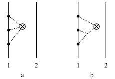
These diagrams are also characterized by the fact that they involve, as post-Minkowskian diagrams (i.e., before explicitly performing the PN expansion, or the repeated time derivatives, which can introduce the acceleration of the world-line), either $m_{1}^{3}$ or $m_{2}^{3}$ as explicit factor. This reasoning is confirmed by a scrutiny of the many explicit results reported in Blanchet et al. (2002a) for separate pieces of the multipole moments. In the presentation of Ref. Blanchet et al. (2002a) (which is less systematic than the more recent re-calculation of Blanchet and Iyer (2004), but more explicit) the dangerously divergent integrals (in $d=3$) are essentially all the terms involving the objects $Y_{L}^{(-3,0)}$, $Y_{L}^{(-5,0)}$ or $S_{L}^{(-5,0)}$, and these terms are all multiplied by $m_{1}^{3}$. Indeed, these objects are integrals of the type $\int d^{3}\mathbf{x}\,r_{1}^{-3}\varphi(\mathbf{x})$ or $\int d^{3}\mathbf{x}\,\Delta(r_{1}^{-3})\,\varphi(\mathbf{x})$, which are logarithmically divergent in $d=3$, and lead to $1/\varepsilon$ poles in $d=3+\varepsilon$.

Let us exhibit the explicit form of the terms, corresponding to the diagrams shown in Fig. 1, which are responsible for the poles $\propto 1/\varepsilon$ in the final result for the multipole moments. Let us decompose, as in Blanchet et al. (2002a); Blanchet and Iyer (2004), the expression for $I_{L}$ in: (i) “first-order scalar” part $\mathrm{SI}_{L}$ (linear in $\Sigma$), (ii) second-order scalar part $\mathrm{SII}_{L}$ (linear in $\partial_{t}^{2}\,\Sigma/c^{2}$), (iii) first-order vector part $\mathrm{VI}_{L}$ (linear in $\partial_{t}\,\Sigma_{i}/c^{2}$), etc. One finds that the “dangerous” contributions to $I_{L}$ are contained only in $\mathrm{SI}_{L}$, $\mathrm{SII}_{L}$ and $\mathrm{VI}_{L}$. Moreover, one finds that the velocity-dependent terms that generates poles $\propto 1/\varepsilon$ in intermediate calculations all cancel out in the final result. We focus here for simplicity on the non-cancelled poles, which do not depend on velocities. Hence,

$$I_{L}^{\mathrm{danger}}=\mathrm{SI}_{L}^{\mathrm{danger}}+\mathrm{SII}_{L}^{\mathrm{danger}}+\mathrm{VI}_{L}^{\mathrm{danger}}\,,$$ (128)

where one checks that among the many contributions generated by inserting Eq. (83) into Eq. (73) the only potentially dangerous ones, in the static limit $\mathbf{v}_{1}\rightarrow 0$, $\mathbf{v}_{2}\rightarrow 0$, come from

$$\mathrm{SI}_{L}^{\mathrm{danger}} = \frac{1}{\pi\,f\,G\,c^{4}}\,\mathrm{FP}\int d^{d}\mathbf{x}\,\widetilde{r}^{B}\,\widehat{x}_{L}\Biggl{\{}-\hat{W}_{ij}\,\partial_{ij}\,V-\frac{1}{6}\left(\frac{d-1}{d-2}\right)^{2}\,\Delta V^{3}-\frac{1}{2}\,\Delta(V\hat{W})$$ (129a)

$$\quad+\frac{1}{c^{2}}\left[\frac{1}{2}\,\hat{W}\,\partial_{t}^{2}\,V+\frac{1}{2}\,V\,\partial_{t}^{2}\,\hat{W}-4\,\hat{Z}_{ij}\,\partial_{ij}\,V+2\,\frac{d-3}{d-2}\,\hat{W}_{ij}\,\partial_{ij}\,K\right]\Biggr{\}},$$

$$\mathrm{SII}_{L}^{\mathrm{danger}} = \frac{1}{2(2\ell+d)\,\pi\,f\,G\,c^{6}}\,\mathrm{FP}\,\frac{d^{2}}{dt^{2}}\int d^{d}\mathbf{x}\,\widetilde{r}^{B}\,\widehat{x}_{L}\biggl{\{}-|\mathbf{x}|^{2}\,\hat{W}_{ij}\,\partial_{ij}\,V$$ (129b)

$$\quad-(2\ell+d)\,V\hat{W}-\frac{1}{3}\,\frac{(2\ell+d)(d-1)^{2}}{(d-2)^{2}}\,V^{3}\biggr{\}},$$

$$\mathrm{VI}_{L}^{\mathrm{danger}} = -\frac{4(2\ell+d-2)}{(\ell+d-2)(2\ell+d)\,\pi\,f\,G\,c^{6}}\,\mathrm{FP}\,\frac{d}{dt}\int d^{d}\mathbf{x}\,\widetilde{r}^{B}\,\widehat{x}_{iL}\,\biggl{\{}\frac{1}{8}\,\frac{d(d-1)^{2}}{(d-2)^{3}}\,V\,\partial_{t}\,V\,\partial_{i}\,V$$ (129c)

$$\quad-\frac{(d-1)^{2}}{4(d-2)^{2}}\,V_{i}\,\partial_{k}\,V\,\partial_{k}\,V+\,\frac{1}{4}\,\frac{d(d-1)}{(d-2)^{2}}\,V_{k}\,\partial_{i}\,V\,\partial_{k}\,V+\frac{d-1}{d-2}\,\partial_{k}\,V\,\partial_{i}\,\hat{R}_{k}$$

$$\quad-\,\hat{W}_{kl}\,\partial_{kl}\,V_{i}+\frac{d-1}{2(d-2)}\,\partial_{t}\,\hat{W}_{ik}\,\partial_{k}\,V-\partial_{i}\,\hat{W}_{kl}\,\partial_{k}\,V_{l}+\,\partial_{k}\,\hat{W}_{il}\,\partial_{l}\,V_{k}\biggr{\}}.$$

where we set $f\equiv\frac{2(d-2)}{d-1}$.

Note that the expression we used for $\mathrm{SII}_{L}$ in our calculations has been transformed, from the original form which is directly arising from the source terms given in Eqs. (83) above, by operating by parts on the terms proportional to $V\hat{W}$ and $V^{3}$. This was done to exactly parallel the calculation of Ref. Blanchet and Iyer (2004) (see for instance Eq. (3.4b) there) and thereby to reduce the problem of evaluating the DR result to a term-by-term difference between analogous singular integrands. As explained in Sec. V.2, all the “gradient terms” generated when operating by parts are expressible in terms of surface integrals in the outer near-zone, and do not contribute to the difference between DR and pHS. We have therefore suppressed most of these gradient terms in Eqs. (129), except in Eq. (129a) where, as an example and as a reminder of the presence of such terms, we have left the terms proportional to the Laplacians of $V^{3}$ and $V\hat{W}$.

Let us explicitly show on the example of $\Delta V^{3}$ that this term, though potentially dangerous, does not give rise to any pole. The linear potential $V$ is naturally decomposed into $V\equiv V_{1}+V_{2}$ where $V_{1}\propto m_{1}$ is generated by the first particle, and $V_{2}\propto m_{2}$ by the second. In agreement with Fig. 1 the dangerous contributions are cubic in $m_{1}$ or cubic in $m_{2}$. In particular, the dangerous pieces in any term containing $V^{3}$ are $(V_{1})^{3}$ and $(V_{2})^{3}$. Let us henceforth look only at the poles generated near the first world-line (i.e., $\propto m_{1}^{3}$). In dimensional regularization, it is perfectly legitimate to integrate by parts. This transforms the contribution $\mathrm{FP}\int d^{d}\mathbf{x}\,\widetilde{r}^{B}\,\widehat{x}_{L}\,\Delta\,V_{1}^{3}$ into $\mathrm{FP}\int d^{d}\mathbf{x}\,\Delta(\widetilde{r}^{B}\,\widehat{x}_{L})\,V_{1}^{3}$. Using $\Delta(r^{B}\,\widehat{x}_{L})=\Delta(r^{B+\ell}\,\widehat{n}_{L})=B(B+2\ell+d-2)\,r^{B+\ell-2}\,\widehat{n}_{L}$, we see that the result is proportional to $B$. As we shall see in detail below the remaining integral $\sim\int d^{d}\mathbf{x}\,\varphi(x)\,V_{1}^{3}$ generates a pole $\propto 1/\varepsilon$. The contribution linear in $\Delta V_{1}^{3}$ yields therefore a result proportional to $B/\varepsilon$. But, by the definition of the $d$-dimensional finite part operation, one has $\mathop{\mathrm{FP}}(B/\varepsilon)=0$, so that we have indeed checked the absence of pole generated by the a priori dangerous term $\propto\Delta V^{3}$. Similarly for the term $\propto\Delta(V\hat{W})$ in (129a).

Let us consider the various remaining terms in the integrand of $\mathrm{SI}_{L}$, Eq. (129a). We start with the term $\propto\hat{W}_{ij}^{\mathrm{NC}}\,\partial_{ij}\,V$, where $\hat{W}_{ij}^{\mathrm{NC}}$ denotes the so-called “non compact” piece of $\hat{W}_{ij}$, i.e., the one whose source is $\sim\partial_{i}\,V\partial_{j}\,V$. Again, it is easily seen that the only dangerous part of the integrand is $\sim\Box^{-1}_{\mathrm{Ret}}(\partial_{i}\,V_{1}\,\partial_{j}\,V_{1})\,\partial_{ij}\,V_{1}$ and its mirror image under the exchange $1\leftrightarrow 2$. [This term is an example of the diagram in Fig. 1b.] We can compute this term by PN-expanding both $V_{1}$ and $\Box^{-1}_{\mathrm{Ret}}$. This yields a result of the form (in the static limit)

$$\mathop{W}_{1}{}_{\!ij}^{\mathrm{\!NC}}\,\partial_{ij}\,V_{1}=\alpha_{0}\,\Delta\,U_{1}^{3}+\frac{\beta_{0}}{c^{2}}\,a_{1}^{k}\,\partial_{k}\,U_{1}^{3}+{\mathcal{O}}(v_{1}^{2})\,,$$ (130)

where $U_{1}=f\,\tilde{k}\,G\,m_{1}\,r_{1}^{-1-\varepsilon}$, with $\tilde{k}\equiv\Gamma(\frac{1+\varepsilon}{2})/\pi^{\frac{1+\varepsilon}{2}}$, is the Newtonian approximation to $V_{1}$, where $a_{1}^{k}\equiv d^{2}\,y_{1}^{k}/dt^{2}$ is the acceleration of the first particle, and where $\alpha_{0}$ and $\beta_{0}$ are numerical coefficients, which depend on $\varepsilon$. By the same reasoning as used above for the term $\propto\Delta V_{1}^{3}$ one concludes that the term $\alpha_{0}\,\Delta\,U_{1}^{3}$ does not generate any pole.

Only the second term on the RHS of (130) generates a pole $\propto 1/\varepsilon$ which survives the finite part operation. By looking at the terms contained in the last bracket on the RHS of Eq. (129a) one finds that the only dangerous integrands have the same form as the second term on the RHS of Eq. (130), namely proportional to $a_{1}^{k}\,\partial_{k}\,U_{1}^{3}$. Let us only give one example of a contribution of this form coming from the last bracket in (129a). Consider the term (which can be treated to leading PN order)

$$\hat{W}^{\mathrm{NC}}\,\partial_{t}^{2}\,V=-f^{-1}\,[\Delta^{-1}(\partial_{k}\,V\,\partial_{k}\,V)]^{\mathrm{NC}}\,\partial_{t}^{2}\,V\,.$$ (131)

From the identity $\partial_{k}V\,\partial_{k}V\equiv\Delta(V^{2}/2)-V\Delta V$ one has $[\Delta^{-1}(\partial_{k}\,V\,\partial_{k}\,V)]^{\mathrm{NC}}=V^{2}/2$, so that the term (131) is of the type of $V^{2}\,\partial_{t}^{2}\,V$. As usual the only dangerous terms are those proportional to $V_{1}^{2}\,\partial_{t}^{2}\,V_{1}$ or $V_{2}^{2}\,\partial_{t}^{2}\,V_{2}$. Focusing on the first one, and using the fact that

$$\partial_{t}^{2}\,V_{1}=-\,a_{1}^{k}\,\partial_{k}\,V_{1}+{\mathcal{O}}(v_{1}^{2})\,,$$ (132)

one ends up with an integrand (131) proportional to $V_{1}^{2}\,a_{1}^{k}\,\partial_{k}\,V_{1}$ or, to leading approximation $U_{1}^{2}\,a_{1}^{k}\,\partial_{k}\,U_{1}$, which is indeed identical to the second term in (130). Finally, we conclude that the dangerous terms in Eq. (129a) are of the form

$$\mathrm{SI}_{L}^{\mathrm{danger}}=\mathop{\mathrm{FP}}\int_{\mathrm{loc}}d^{d}\mathbf{x}\,|\tilde{\mathbf{x}}|^{B}\,\widehat{x}_{L}\left\{\frac{\beta_{\mathrm{SI}}}{\pi\,G\,c^{6}}\,a_{1}^{k}\,\partial_{k}\,U_{1}^{3}\right\},$$ (133)

where $\beta_{\mathrm{SI}}$ is a numerical coefficient which sums several similar contributions: $\beta_{\mathrm{SI}}=-\beta_{0}+\cdots$ [we include the factor $f^{-1}=1+\mathcal{O}(\varepsilon)$ into these coefficients], and where the subscript “loc” to the integral reminds us that one can integrate on any local neighborhood of $\mathbf{x}=\mathbf{y}_{1}$.

Let us now consider the dangerous terms in $\mathrm{SII}_{L}$, Eq. (129b). In this case one must pay a careful attention to the dependence of the coefficients on the angular momentum index $\ell$. Indeed, it is important to note that there was no explicit dependence on $\ell$ in Eq. (133) apart from the factor $\widehat{x}_{L}$. By contrast, the coefficients entering (129b) explicitly depend on $\ell$. Since (129b) has an overall factor $c^{-6}$, it is sufficient to use the leading PN approximations for $\hat{W}_{ij}$ and $V$; in view of our previous (1PN-accurate) result (130) this means that we can use $\hat{W}_{ij}\,\partial_{ij}\,V_{1}\simeq\alpha_{0}\,\Delta\,U_{1}^{3}$ (as usual we focus on the terms $\propto m_{1}^{3}$). The occurrence of an explicit Laplacian allows us to re-express the first term on the RHS of (129b) by integrating by parts. This leads to a term proportional to (we keep only the coefficients depending on $\ell$)

$$\frac{1}{2\ell+d}\mathrm{FP}\,\frac{d^{2}}{dt^{2}}\int d^{d}\mathbf{x}\,\Delta\left(|\widetilde{\mathbf{x}}|^{B}\,|\mathbf{x}|^{2}\,\widehat{x}_{L}\right)\,U_{1}^{3}\,.$$ (134)

Using $\Delta\left(|\mathbf{x}|^{B+2}\,\widehat{x}_{L}\right)=(B+2)(B+2\ell+d)\,|\mathbf{x}|^{B}\,\widehat{x}_{L}$ we get a contribution of the form

$$\frac{1}{\pi\,G\,c^{6}}\,\mathrm{FP}\,\frac{d^{2}}{dt^{2}}\int d^{d}\mathbf{x}\,|\widetilde{\mathbf{x}}|^{B}\,\frac{(B+2)(B+2\ell+d)}{2\ell+d}\,\widehat{x}_{L}\,U_{1}^{3}\,.$$ (135)

The pole part $\propto 1/\varepsilon$ of the contribution (135) is generated by integrating in the vicinity of the first world-line. For such a local integral the IR-converging factor $|\widetilde{\mathbf{x}}|^{B}$ has no importance and we can take the analytic continuation $B\rightarrow 0$ directly in the (localized) integrand. This leads to the disappearance of the $\ell$-dependence in the factor appearing in (135). As for the last two terms on the RHS of (129b), one sees that the $\ell$-dependence cancels between the factor $\propto 1/(2\ell+d)$ in front, and the factors $\propto(2\ell+d)$ multiplying the integrands $\widehat{x}_{L}\,V\hat{W}$ and $\widehat{x}_{L}\,V^{3}$. Finally, we conclude that the dangerous terms in $\mathrm{SII}_{L}$ are of the form

$$\mathrm{SII}_{L}^{\mathrm{danger}}=\frac{d^{2}}{dt^{2}}\int_{\mathrm{loc}}d^{d}\mathbf{x}\,\widehat{x}_{L}\left\{\frac{\beta_{\mathrm{SII}}}{\pi\,G\,c^{6}}\,U_{1}^{3}\right\}+{\mathcal{O}}(v_{1}^{2})\,.$$ (136)

The coefficient $\beta_{\mathrm{SII}}$ does not depend on $\ell$ (like was the case for $\beta_{\mathrm{SI}}$). The repeated time derivative in (136) can then be let to act on $U_{1}^{3}$ only (modulo “non dangerous” terms) yielding, in view of Eq. (132), $\partial_{t}^{2}\,U_{1}^{3}\simeq-\,a_{1}^{k}\,\partial_{k}\,U_{1}^{3}$ so that

$$\mathrm{SII}_{L}^{\mathrm{danger}}=\int_{\mathrm{loc}}d^{d}\mathbf{x}\,\widehat{x}_{L}\left\{-\,\frac{\beta_{\mathrm{SII}}}{\pi\,G\,c^{6}}\,a_{1}^{k}\,\partial_{k}\,U_{1}^{3}\right\}.$$ (137)

A similar study of the “vector” contribution $\mathrm{VI}_{L}$, Eq. (129c), yields a result of the form

$$\frac{1}{\pi\,G\,c^{6}}\,\frac{(2\ell+d-2)}{(\ell+d-2)(2\ell+d)}\,\mathrm{FP}\int_{\mathrm{loc}}d^{d}\mathbf{x}\,|\widetilde{\mathbf{x}}|^{B}\,\widehat{x}_{iL}\Bigl{\{}\alpha_{\mathrm{VI}}\,a_{1}^{i}\,\Delta\,U_{1}^{3}+\beta_{\mathrm{VI}}\,a_{1}^{k}\,\partial_{ik}\,U_{1}^{3}\Bigr{\}}.$$ (138)

Integrating by parts the first term, and taking the finite part at $B=0$ is easily seen to give a vanishing result [because $\Delta(\widehat{x}_{iL})=0$]. The second term of (138), with a coefficient denoted $\beta_{\mathrm{VI}}$, is a priori more problematic. Integrating by parts does not give a vanishing result (because $\partial_{i}\,\widehat{x}_{iL}\propto\widehat{x}_{L}$ does not vanish). If present this term would have a complicated dependence on $\ell$. However, the overall coefficient $\beta_{\mathrm{VI}}$ of this term is the sum of many individual contributions, and one finds that they all cancel out to yield $\beta_{\mathrm{VI}}=0$, so that finally

$$\mathrm{VI}_{L}^{\mathrm{danger}}=0\,.$$ (139)

The result $\beta_{\mathrm{VI}}=0$ can be obtained either by explicit calculations in $d$ dimensions, using notably the explicit form of $\hat{W}_{ij}^{\mathrm{NC}}$, namely (to leading order)

$$\mathop{\hat{W}}_{1}{}_{\!ij}^{\mathrm{\!NC}}=-\,\frac{1}{4}\,(d-1)(d-2)\,U_{1}^{2}\,\left[\frac{\widehat{n}_{1}^{ij}}{(d-1)(d-4)}+\frac{\delta^{ij}}{d(d-2)^{2}}\right],$$ (140)

or by considering the limiting case $d=3$. In this limiting case, the poles $\propto 1/\varepsilon$ are associated to logarithmically divergent integrals. Looking at the 3-dimensional results given by (8.2c), (9.3j) and (9.3k) of Ref. Blanchet et al. (2002a) for $\mathrm{VI}_{L}$, one indeed finds that the terms $a_{1}^{k}\,\partial_{ik}\,Y_{iL}^{(-3,0)}$, corresponding to the $d=3$ limit of the second contribution in (138), do cancel in the final result, though they appear in intermediate terms: see the first terms on the RHS of Eqs. (9.3j)–(9.3k) of Blanchet et al. (2002a) with coefficients $+2/63$ and $-2/63$ respectively (note a small misprint in (9.3k) of Blanchet et al. (2002a): the overall factor $m_{1}^{2}$ should be understood as $m_{1}^{3}$). Note also that, in view of the general structure (138) derived above, it is enough to check the cancellation of these terms for the quadrupolar case $(\ell=2)$ to conclude that $\beta_{\mathrm{VI}}=0$.

Summarizing our results so far, we conclude, by adding (133), (137) and (139) that the pole part $\propto m_{1}^{3}$ in the $\ell$-th mass multipole moment is contained in

$$I_{L}^{\mathrm{danger}}=\int_{\mathrm{loc}}d^{d}\mathbf{x}\,\widehat{x}_{L}\left\{\frac{\beta}{\pi\,G\,c^{6}}\,a_{1}^{k}\,\partial_{k}\,U_{1}^{3}\right\},$$ (141)

with a final coefficient $\beta=\beta_{\mathrm{SI}}-\beta_{\mathrm{SII}}$. By summing the various contributions one finds

$$\beta=-\frac{11}{6}+{\mathcal{O}}(\varepsilon)\,,$$ (142)

where the first term on the RHS is enough to discuss the residue of the pole $\propto 1/\varepsilon$.

VII.2 Renormalization of poles by shifts of the world-lines

The result (141)–(142) is the explicit expression of the dangerous part of the two diagrams of Fig. 1. Let us now see explicitly why it is nicely renormalized away by using exactly the same dipole counter-term that was found necessary in Blanchet et al. (2004a). The pole generated by (141) can be seen, after integrating by parts the spatial gradient ($\partial_{k}$), as coming from an integral of the form

$$I_{\mathrm{loc}}=\int_{\mathrm{loc}}d^{d}\mathbf{x}\,\varphi(\mathbf{x})\,U_{1}^{3}\,,$$ (143)

where $\varphi(\mathbf{x})$ is a smooth function of $\mathbf{x}$ (at least near $\mathbf{x}=\mathbf{y}_{1}$). Taylor-expanding $\varphi(\mathbf{x})$ near $\mathbf{x}=\mathbf{y}_{1}$ one sees that the pole in (143) comes from the zero-th term $\varphi(\mathbf{y}_{1})$ which multiplies an integral proportional to

$$\int_{\mathrm{loc}}d^{3+\varepsilon}\mathbf{x}\,r_{1}^{-3-3\varepsilon}=\Omega_{2+\varepsilon}\int_{0}^{R}dr_{1}\,r_{1}^{-1-2\varepsilon}=\Omega_{2+\varepsilon}\,R^{-2\varepsilon}/(-2\varepsilon)\,,$$ (144)

where we recall that $\Omega_{2+\varepsilon}$ denotes the area of the $2+\varepsilon$ dimensional sphere. Therefore, in the limit $\varepsilon\rightarrow 0$, the integral (143) is asymptotically equivalent to

$$I_{\mathrm{loc}}=-\,\frac{2\pi}{\varepsilon}\,G^{3}\,m_{1}^{3}\,\varphi(\mathbf{y}_{1})+\mathcal{O}\left(\varepsilon^{0}\right).$$ (145)

This means that, when $\varepsilon\rightarrow 0$ the integrand $U_{1}^{3}$ is asymptotically equivalent (in the formal sense of distributions in $d$-dimensional space) to

$$U_{1}^{3}=-\,\frac{2\,\pi}{\varepsilon}\,G^{3}\,m_{1}^{3}\,\delta(\mathbf{x}-\mathbf{y}_{1})+{\mathcal{O}}\left(\varepsilon^{0}\right).$$ (146)

Inserting this result into (141) one concludes that the pole part (due to the UV divergencies in the neighborhoods of $\mathbf{y}_{1}$ and $\mathbf{y}_{2}$) of the 3PN-accurate $\ell$-th mass multipole moment is given by

$$I_{L}^{\mathrm{pole}}=\int d^{d}\mathbf{x}\,\widehat{x}_{L}\,a_{1}^{k}\,\partial_{k}\left\{-\,\frac{2\beta}{\varepsilon}\,\frac{G^{2}\,m_{1}^{3}}{c^{6}}\,\delta(\mathbf{x}-\mathbf{y}_{1})\right\}+1\leftrightarrow 2\,.$$ (147)

If we compare (147) with the leading, Newtonian approximation for $I_{L}$, namely

$$I_{L}^{\mathrm{N}}=\int d^{d}\mathbf{x}\,\widehat{x}_{L}\,\Bigl{\{}m_{1}\,\delta(\mathbf{x}-\mathbf{y}_{1})\Bigr{\}}+1\leftrightarrow 2\,,$$ (148)

we see that the pole part (147) can be absorbed in a dipole-like modification [$\sim\partial_{k}\,\delta(\mathbf{x}-\mathbf{y}_{1})$] of the mass density $m_{1}\,\delta(\mathbf{x}-\mathbf{y}_{1})$, or equivalently in a shift of the world-line position $\mathbf{y}_{1}$. More precisely, if we decompose the full $\mathbf{y}_{1}$ (henceforth called the “bare” $\mathbf{y}_{1}$) as in Eq. (127), with $\mathbf{y}_{1}^{\mathrm{ren}}$ being finite as $\varepsilon\rightarrow 0$, but with $\bm{\eta}_{1}$ designed to absorb the pole part (147), one easily checks that one needs to define

$$\eta_{1}^{k}=-\frac{2\beta}{\varepsilon}\,\frac{G^{2}\,m_{1}^{2}}{c^{6}}\,a_{1}^{k}+{\mathcal{O}}(\varepsilon^{0})\,,$$ (149)

in order to renormalize away this pole. Note that it was crucial to have no $\ell$-dependence of the coefficients in the dangerous part (141) in order to be able to renormalize away the infinite sequence of multipoles by means of the $\ell$-independent shift $\bm{\eta}_{1}$ (149).

In addition, by inserting the numerical value (142) of the coefficient $\beta$, one finds that the shift (149) needed to absorb the poles in the infinite sequence of multipole moments coincides with the shift obtained in Blanchet et al. (2004a) by the requirement of renormalizing both the “bulk metric” and the equations of motion. More precisely, Ref. Blanchet et al. (2004a) found that the choice of the shift recalled above in Eq. (110) [and which contains (149) as its pole part] allowed one not only to get a finite (pole-less) bulk metric and finite equations of motion, but that the equations of motion coincide (when, and only when, $\lambda=-1987/3080$) with the harmonic-gauge equations of motion, parametrized by $r^{\prime}_{1}$ and $r^{\prime}_{2}$, and derived using HR in Refs. Blanchet and Faye (2000a, 2001). We recall that it is necessary to introduce some length scales $r^{\prime}_{1}$ and $r^{\prime}_{2}$ associated with the HR of logarithmically divergent integrals in harmonic gauge.

As we have shown here the dangerous divergencies associated with the vicinity of the first world-line are entirely contained in the diagrams shown in Fig. 1, and, therefore, are proportional to $m_{1}^{3}$, without any explicit dependence on the second mass $m_{2}$. [There is only an implicit dependence on $m_{2}$ via the fact that the acceleration $\mathbf{a}_{1}$ is proportional to $m_{2}$. But, at the level of the diagrams, $\mathbf{a}_{1}$ must be considered as a pure characteristic of the first world-line.] As a consequence, we see in Eq. (149) that the dipole $m_{1}\eta_{1}^{k}$ needed to subtract the poles is also proportional to $m_{1}^{3}$. This simple algebraic fact immediately leads, without calculations, to the result that $\kappa=0$. Indeed, the definition of the parameter $\kappa$ in Ref. Blanchet et al. (2002a), was to parametrize a conceivable a priori ambiguity, which is indeed allowed by the weak assumptions of Blanchet et al. (2002a), in the renormalization of the logarithmic divergencies of the type (for the first particle)

$$m_{1}^{3}\,\ln\left(\frac{r^{\prime}_{1}}{s_{1}}\right)=\left(\xi+\kappa\right)\,m_{1}^{3}+\kappa\,m_{1}^{2}\,m_{2}\,,$$ (150)

where $r^{\prime}_{1}$ and $s_{1}$ are two possible choices of regularization length scales associated to the first particle, and where we have incorporated the factor $m_{1}^{3}$ associated to the divergences linked to $\mathbf{y}_{1}$. As (150) shows, the parameter $\kappa$ corresponds to a mixing between diagrams with three legs on the first world-line (as in Fig. 1) and diagrams having two legs on the first world-line and one on the second. Our diagrammatic study has shown that the latter diagrams have no dangerous divergencies, i.e., that they do not introduce any conceivable ambiguity (even if we were working directly in $d=3$, using HR). Therefore we conclude that $\kappa=0$.

The work of this section has shown that the pole in the $\ell$-th mass moment $I_{L}$ was given by Eq. (147) whose numerical coefficients contain no dependence on the value of $\ell$. This proves, in particular, that the same shift (149), or more precisely (110), yields finite values of both the quadrupole moment $I_{ij}$ ($\ell=2$) and the dipole moment $M_{i}$ ($\ell=1$). As said above the mass dipole moment $M_{i}$ coincides with the Arnowitt-Deser-Misner (ADM) dipole moment or center-of-mass position $G_{i}$, such that $G_{i}-P_{i}\,t$ is conserved, where $P_{i}$ denotes the total ADM linear momentum. The comparison between $M_{i}$ and $G_{i}$ in Blanchet and Iyer (2004) permitted to fix the value of the combination $\xi+\kappa=-9871/9240$ within the HR scheme, under the assumption that the regularization scales $s_{1}$ and $s_{2}$ represent some unknown but fixed constants, related to $r^{\prime}_{1}$ and $r^{\prime}_{2}$ by some definite equations, and in particular take the same values for both the computations of the quadrupole $I_{ij}$ and the dipole $M_{i}$. This assumption worked well in the case of the HR computation of the multipole moments, but failed to work when it was tried to assume that the same scales $s_{1}$ and $s_{2}$ are also those which entered the HR computation of the equations of motion Blanchet and Faye (2001). Indeed, the work on the equations of motion used for the relation between $s_{1}$ and $r^{\prime}_{1}$, for the divergences linked to the first particle, $\ln(r^{\prime}_{1}/s_{1})=\mathrm{const}+\lambda\,m_{2}/m_{1}$ where $\lambda$ was later determined to have a non-zero value, $\lambda=-1987/3080$. Such a link is clearly incompatible with (150) and the value we have found for $\kappa=0$. This means that one is not a priori allowed to assume, when using HR, that the scales $s_{1}$ and $s_{2}$ represent always the same scales, fixed once and for all, and which can be used in different bodies of calculations. In this respect the HR is not a fully consistent regularization scheme. However, it can nevertheless be applied if one accepts that its incompleteness results in the appearance of some unknown scales $s_{1}$ and $s_{2}$ (generally in front of a few terms only), which can take different values, depending on the type of calculation one is doing. By contrast we have proved in Sec. VI.2 above that the same value of $\xi$ is consistent, in DR, with the renormalized results of both $I_{ij}$ and $M_{i}=G_{i}$. This result constitutes evidently a solid confirmation of the value $\xi=-9871/9240$.

VII.3 Comments on finite-size effects in the effective action of compact bodies

To conclude our discussion of the diagrammatic approach to the renormalization of the poles which appear in harmonic gauge, let us briefly comment on the recent claim Goldberger and Rothstein (2004) that these poles require the introduction of new terms in the effective action describing compact (but extended) objects, beyond Eq. (126) and the dipole term we found above, linked to the shift (127). The modified effective action proposed in Ref. Goldberger and Rothstein (2004) has the form

$$S^{\prime}_{\mathrm{pp}}=S_{\mathrm{pp}}+S_{\mathrm{finite\,size}}\,,$$ (151)

where $S_{\mathrm{pp}}$ is the standard point-particle effective action (126) and where

$$S_{\mathrm{finite\,size}}=\sum_{a}c_{R}^{(a)}\!\!\int ds_{a}\,R(y_{a})+\sum_{a}c_{V}^{(a)}\!\!\int ds_{a}\,R_{\mu\nu}(y_{a})\,u_{a}^{\mu}\,u_{a}^{\nu}\,,$$ (152)

with $u_{a}^{\mu}\equiv dy_{a}^{\mu}/ds_{a}$. Several claims were made in Ref. Goldberger and Rothstein (2004): (i) that the extra terms (152) are necessary to “encapsulate finite size properties of the sources”, (ii) that they are linked to the same “dangerous” diagrams that were examined in Fig. 6 of Blanchet et al. (2004a) and Fig. 1 above, and (iii) that they entail the presence of genuine ambiguities at the 3PN level which can only be fixed by a matching calculation. If these statements were correct, that would mean not only that the basic “effacement” property (modulo 5PN-level “quadrupole-type” additional terms to the effective action) is incorrect, but also that the recent results, Damour et al. (2001b); Blanchet et al. (2004a, b) and this work, fixing all 3PN-level ambiguity parameters by DR are flawed.

Let us, however, indicate why we think that the claims (i), (ii) and (iii) made in Ref. Goldberger and Rothstein (2004) are not correct. First, we mention that the addition of curvature-coupling terms of the type indicated in (152) has already been considered in Ref. Nordtvedt (1994) and in Appendix A of Ref. Damour and Esposito-Farèse (1998), which considered finite-size effects in tensor-scalar gravity. Indeed, when gravity is partly mediated by a scalar excitation, the internal characteristics of compact objects are much less effaced than in the pure spin-2 case. In particular, the coupling to the spherical inertia moment $I\sim\int d^{3}\,\mathbf{x}\,\sigma(\mathbf{x})\,\mathbf{x}^{2}$ can introduce extra couplings of the type of the curvature terms in (152) (see Nordtvedt (1994)) together with several other scalar-dependent couplings. However, it was shown in Damour and Esposito-Farèse (1998) that the use of suitable field redefinitions can transform away the curvature couplings (152) into couplings explicitly involving the gradient of the scalar field, $\int ds_{a}\,N_{a}(\varphi)\,g^{\mu\nu}\,\partial_{\mu}\,\varphi\,\partial_{\nu}\,\varphi$. As such a term does not exist in the pure spin-2 case, one sees that Ref. Damour and Esposito-Farèse (1998) proves that (152) can be field-redefined away. Indeed, a simple way to see it is to recall that the first-order effect of a field redefinition of the metric $(g^{\prime}_{\mu\nu}=g_{\mu\nu}+\varepsilon\,h_{\mu\nu})$ is to modify the effective action by terms proportional to the Einstein field equations, namely $\delta\,S_{\mathrm{tot}}=-(16\,\pi\,G)^{-1}\int d^{D}x\,\sqrt{-g}\,(R^{\mu\nu}-\frac{1}{2}\,R\,g^{\mu\nu}-8\,\pi\,G\,T^{\mu\nu})\,\varepsilon\,h_{\mu\nu}$ [to simplify, we set the light velocity $c=1$ here and below]. Conversely, the (a priori illicit) use of the Einstein field equations within an action is equivalent to a suitably defined field redefinition $\varepsilon\,h_{\mu\nu}$. Applying this general result to (151) we see that the curvature coupling terms (152) are equivalent to

$$S^{\prime}_{\mathrm{finite\,size}} = \sum_{a}c^{\prime(a)}_{R}\!\!\!\int\!\!\!\!\int\!ds_{a}\,ds^{\prime}_{a}\,\frac{m_{a}}{\sqrt{-g}}\,\delta^{(D)}(y_{a}^{\mu}(s_{a})-y_{a}^{\mu}(s^{\prime}_{a}))$$ (153)

$$+ \sum_{a}c^{\prime(a)}_{V}\!\!\!\int\!\!\!\!\int\!ds_{a}\,ds^{\prime}_{a}\,\frac{m_{a}}{\sqrt{-g}}\,u_{a}^{\mu}(s_{a})\,u_{a}^{\nu}(s_{a})\,u_{a\mu}(s^{\prime}_{a})\,u_{a\nu}(s^{\prime}_{a})\,\delta^{(D)}(y_{a}^{\mu}(s_{a})-y_{a}^{\mu}(s^{\prime}_{a}))\qquad\quad$$

(where $D=d+1$ and $u_{a}^{\mu}\equiv dy_{a}^{\mu}/ds_{a}$) modulo a field redefinition $g^{\prime}_{\mu\nu}=g_{\mu\nu}+h_{\mu\nu}$ of the type

$$h_{\mu\nu}(x)=\sum_{a}\int ds_{a}\,[c^{\prime\prime(a)}_{R}\,g_{\mu\nu}+c^{\prime\prime(a)}_{V}\,u_{\mu}\,u_{\nu}]\,\frac{\delta^{(D)}(x^{\lambda}-y_{a}^{\lambda}(s_{a}))}{\sqrt{-g}}\,.$$ (154)

Here $c^{\prime}_{R}$, $c^{\prime}_{V}$, $c^{\prime\prime}_{R}$, $c^{\prime\prime}_{V}$ are linear combinations of the coefficients $c_{R}$, $c_{V}$ entering (152), namely $c^{\prime\prime}_{R}=-2c^{\prime}_{R}=16\pi G(c_{V}-2c_{R})/(d-1)$, $c^{\prime\prime}_{V}=2c^{\prime}_{V}=16\pi Gc_{V}$. After using, for instance, the delta function in time, $\delta(y_{a}^{0}(s_{a})-y_{a}^{0}(s^{\prime}_{a}))$, to integrate over $s^{\prime}_{a}$ (with the conclusion that $s^{\prime}_{a}=s_{a}$), one easily sees that the result (153) is proportional to the $s_{a}$-integral of the $d$-dimensional delta function evaluated at a vanishing separation: $\delta^{(d)}(y_{a}^{i}(s_{a})-y_{a}^{i}(s_{a}))$. In DR, such a pure contact term vanishes exactly, so that we have simply $S^{\prime}_{\mathrm{finite\,size}}=0$. [As Ref. Goldberger and Rothstein (2004) uses also DR, we are entitled in using DR to discuss their claims.] Therefore we conclude that the proposed curvature-coupling terms (152) are equivalent to a field redefinition of the type (154). However, (154) is again a “contact term” in the sense that it vanishes outside of the world-lines, and cannot therefore affect the external field generated by the world-lines that we are interested in. In conclusion, the term (152) can be essentially completely field-redefined away, and has no physical import.

We can give another (partial) confirmation of this result by looking at the form of the pole that Ref. Goldberger and Rothstein (2004) claims to be associated with the diagrams in Fig. 6 of Blanchet et al. (2004a), or Fig. 1 here (i.e., diagrams (c) and (d) of Fig. 7 of Goldberger and Rothstein (2004)). Transcribing the Fourier-space result (53) of Goldberger and Rothstein (2004) in $x$-space, and considering the combination that enters the leading term in the multipole moments, one finds that, according to Goldberger and Rothstein (2004), those dangerous diagrams are equivalent, when $\varepsilon\rightarrow 0$, to an effective mass-energy distribution of the type

$$\Sigma_{\mathrm{eff}}^{\text{Gold.-Roth.}}\equiv\frac{T_{(3)}^{00}+T_{(3)}^{ii}}{c^{2}}=\frac{Q}{\varepsilon}\,\frac{G^{2}\,m_{1}^{3}}{c^{4}}\,\Delta\,\delta(\mathbf{x}-\mathbf{y}_{1})\,,$$ (155)

where $Q$ is a (non zero) numerical constant and $\Delta$ the Laplacian.

The result (155) is consistent with part of our analysis above. Indeed, using Eqs. (130), (133), (138) and (146), our analysis has shown that the dangerous terms in the cubically non-linear “non compact” contributions to $\Sigma$, $\Sigma_{i}$ and $\Sigma_{ij}$ are equivalent to a term in $\Sigma$ of the form

$$\Sigma_{\mathrm{eff}}=\frac{1}{\varepsilon}\,\frac{G^{2}\,m_{1}^{3}}{c^{4}}\left[\alpha\,\Delta\,\delta(\mathbf{x}-\mathbf{y}_{1})+\frac{\beta}{c^{2}}\,a_{1}^{k}\,\partial_{k}\,\delta(\mathbf{x}-\mathbf{y}_{1})\right].$$ (156)

The equation (155) is consistent with the first term on the RHS of (156). But, as we have shown above, this term has no physical implication; only the second term, involving a dipole coupling $a_{1}^{k}\,\partial_{k}\,\delta$, mattered. This confirms our conclusion that the claims (i), (ii) and (iii) of Goldberger and Rothstein (2004) are not correct because the terms they considered have no physical relevance. Note also that the “finite size” effect (155) (formally linked to a spherical inertia moment $\int d^{3}\,\mathbf{x}\,\sigma(\mathbf{x})\,\mathbf{x}^{2}$, as in the tensor-scalar case of Damour and Esposito-Farèse (1998)) is actually a 2PN-level term. If that term had created physical effects linked to the finite-size of the source, this would have meant that the 2.5PN equations of motion Damour (1983) had missed some 2PN violation of the effacement properties. As a final comment let us recall that the ADM-gauge calculations of Damour et al. (2001b) never exhibited any pole. In ADM-gauge all the 3PN diagrams are finite and the whole discussion of possible Renormalization-Group dependent quantities evaporates away.

VIII Quadrupole moment of a boosted point particle

In Sec. VI we obtained unique values for the three heretofore unknown parameters $\xi$, $\kappa$ and $\zeta$, by adding to the HR calculations of the quadrupole moment of an interacting binary point-mass system the additional contributions $\mathcal{D}I_{ij}$ coming from a DR treatment of the singularities near $\mathbf{y}_{1}$ and $\mathbf{y}_{2}$. In Sec. VII we have shown that a detailed study of the structure of the singular diagrams represented in Fig. 1 allowed one to check the values of both $\kappa$ and $\xi$ (using information about the full computation of the dipole moment in HR to check the latter). Here, we shall complete our checks by giving an independent calculation of the third parameter $\zeta$. This calculation will be based on a full DR evaluation of the quadrupole moment of a moving isolated particle ($m_{1}\neq 0$, $m_{2}=0$). In another paper, Ref. Blanchet et al. (2005), we have already checked the value of $\zeta$ within a purely $3$-dimensional approach, based on the physical situation of an isolated boosted Schwarzschild (exterior) solution with mass $m_{1}$ (and still with $m_{2}=0$), and without use of any self-field regularization. Therefore our new, DR-based, computation of $\zeta$ given here can also be viewed as a further check of the consistency of DR.

We thus consider the limiting case of a single particle with mass $m_{1}$, moving on a straight line. In order to be able to discuss meaningfully this limiting case, it is important not to use a center-of-mass frame for the original binary system $m_{1}$, $m_{2}$. Indeed, if we start from a center-of-mass frame before taking the limit $m_{2}\rightarrow 0$, we shall end up with a single particle at rest and placed at the center of the coordinate frame used to compute the multipole moments. To simplify the notation, we shall suppress the index $1$ on the characteristics of the single particle that we consider. As in Blanchet et al. (2005) we gain also some simplification by assuming that the origin of the coordinate system (with respect to which the particle is moving) which is used to define the multipole moments coincides with the position of the particle at the time $t=0$. In other words, we consider a single particle of mass $m$, moving on the world-line $y^{i}=v^{i}t$. As was already used in Blanchet et al. (2005), the limiting case $m_{1}\rightarrow m$, $m_{2}\rightarrow 0$, $y_{1}^{i}\rightarrow y^{i}=v^{i}t$ of the mass-type quadrupole moment of a binary system $I_{ij}(m_{1},m_{2})$, evaluated by HR in Blanchet et al. (2002a); Blanchet and Iyer (2004), takes the form (at 3PN order)

$$I_{ij}^{\mathrm{HR}}(m,0)=m\,y^{\langle i}y^{j\rangle}\left[1+\frac{9}{14}\,\frac{v^{2}}{c^{2}}+\frac{83}{168}\,\frac{v^{4}}{c^{4}}+\frac{507}{1232}\,\frac{v^{6}}{c^{6}}\right]+\left(\frac{232}{63}+\frac{44}{3}\,\zeta\right)\frac{G^{2}m^{3}}{c^{6}}\,v^{\langle i}v^{j\rangle}\,.$$ (157)

As we see, the $\zeta$-ambiguity enters only in a term $\propto G^{2}m^{3}v^{\langle ij\rangle}/c^{6}$. We shall henceforth focus on this term and show how DR uniquely fixes its coefficient, i.e., the numerical coefficient $\mathcal{C}$ in the expression

$$I_{ij}^{\mathrm{DR}}(m,0)=\mathcal{B}\,m\,y^{\langle i}y^{j\rangle}+\mathcal{C}\,\frac{G^{2}m^{3}}{c^{6}}v^{\langle i}v^{j\rangle}\,.$$ (158)

To evaluate the coefficient $\mathcal{C}$ in DR, the first step is to obtain the $D$-dimensional metric, in harmonic coordinates, generated by a boosted point particle. We shall first determine the metric generated by a point particle at rest and then apply Lorentz invariance in $D$ dimensions. There are two ways of doing this. We can start from the expressions for the harmonically relaxed Einstein field equations (at 3PN order) explicitly given in Blanchet et al. (2004a) and solve them by iteration, when assuming a source given by a single delta function. Another method consists in starting from the well-known $D$-dimensional Schwarzschild solution, in Schwarzschild-Droste coordinates, and then look for the particular harmonic coordinates selected by the DR treatment of delta-function sources. We have used both methods and checked that they fully agree. Let us indicate some details of the first, more pedestrian, approach.

In the rest frame of a single point particle, the stress-energy tensor has $T^{00}=m\,c^{2}\delta^{(d)}(\mathbf{x})$ as single non-vanishing component. This yields a “scalar” source $\sigma(\mathbf{x})$, as used in our formalism, see Eq. (77), of the form

$$\sigma(\mathbf{x})=f\,m\,\delta^{(d)}(\mathbf{x})\,,$$ (159)

with $f\equiv 2(d-2)/(d-1)$, together with $\sigma_{i}=0=\sigma_{ij}$. The basic scalar potential $V$ generated by $\sigma$, $\Box V=-4\pi G\sigma$, is then found to be

$$V=f\,\tilde{k}\,\frac{G\,m}{r^{d-2}}\,,$$ (160)

where $\tilde{k}\equiv\Gamma[(d-2)/2]/\pi^{(d-2)/2}$. The other linear potentials are easily found to vanish, $V_{i}=0$, $K=0$. Going then to the various non-linear potentials, one finds, successively, $\hat{R}_{i}=0$, $\hat{Z}_{ij}=0$, $\hat{Y}_{i}=0$, as well as $\hat{T}=0$. Note that the vanishing of all those potentials results both from the treatment of contact terms in DR (namely $r^{\alpha}\delta^{(d)}(\mathbf{x})=0$) and from the special structure of Einstein’s equations (the fact that $\hat{Z}_{ij}$ and $\hat{T}$ vanish is due to the special structure of some cubic non-linearities in Einstein’s equations). Finally, besides $V$, the only non-vanishing potentials are $\hat{W}_{ij}$ and $\hat{X}$, which are determined by solving

$$\Delta\hat{W}_{ij} = -\frac{1}{2}\left(\frac{d-1}{d-2}\right)\partial_{i}V\partial_{j}V\,,$$ (161a)

$$\Delta\hat{X} = \hat{W}_{ij}\partial_{ij}V\,.$$ (161b)

As in Blanchet et al. (2004a), it is useful to introduce the combination

$$\mathcal{V}\equiv V-\frac{2}{c^{2}}\left(\frac{d-3}{d-2}\right)K+\frac{4}{c^{4}}\hat{X}+\frac{16}{c^{6}}\hat{T}=V+\frac{4}{c^{4}}\,\hat{X}\,,$$ (162)

which simplifies the expression of the metric. Indeed, one has

$$g_{00} = -\exp\left(-2\frac{\mathcal{V}}{c^{2}}\right)+\mathcal{O}\left(\frac{1}{c^{10}}\right),$$ (163a)

$$g_{ij} = \exp\left(\frac{2}{d-2}\,\frac{\mathcal{V}}{c^{2}}\right)\left\{\delta_{ij}+\frac{4}{c^{4}}\,W_{ij}\right\}+\mathcal{O}\left(\frac{1}{c^{8}}\right),$$ (163b)

and $g_{0i}=0$. The “gothic” metric $\mathfrak{g}^{\mu\nu}\equiv\sqrt{-g}\,g^{\mu\nu}$ reads, besides $\mathfrak{g}^{0i}=0$,

$$\mathfrak{g}^{00} = -\exp\left(2\,\frac{d-1}{d-2}\,\frac{\mathcal{V}}{c^{2}}\right)\left\{1+\frac{2}{c^{4}}\,\hat{W}_{kk}\right\}+\mathcal{O}\left(\frac{1}{c^{8}}\right),$$ (164a)

$$\mathfrak{g}^{ij} = \delta_{ij}-\frac{4}{c^{4}}\,\hat{W}_{ij}+\frac{2}{c^{4}}\,\hat{W}_{kk}\delta_{ij}+\mathcal{O}\left(\frac{1}{c^{8}}\right).$$ (164b)

Note that a remarkable simplification occurred in the expression (164b) of the spatial gothic metric. Indeed, we see form (160) that $V/c^{2}$ is proportional to $Gm/c^{2}$ and therefore that $\hat{W}_{ij}/c^{4}\propto(Gm/c^{2})^{2}$ while $\hat{X}/c^{6}\propto(Gm/c^{2})^{3}$. The result (164b) shows that $\mathfrak{g}^{ij}=\delta^{ij}+\mathcal{O}[(Gm/c^{2})^{2}]+\mathcal{O}[(Gm/c^{2})^{4}]+\cdots$. The point is that there are no terms $\propto(Gm/c^{2})^{3}$ in the spatial gothic metric. One can even prove, more generally, that the spatial structure of Einstein’s equations is such that $\mathfrak{g}^{ij}$ (for a particle at rest) contains only even powers of $Gm/c^{2}$. The only component of the gothic metric which contains odd powers of $Gm/c^{2}$, and in particular $(Gm/c^{2})^{3}$, is the time-time component $\mathfrak{g}^{00}$, Eq. (164a).

By explicitly solving Eq. (161a), we find, in $d$ dimensions,

$$\hat{W}_{ij}=-\frac{1}{4}(d-1)(d-2)V^{2}\left[\frac{\widehat{n}_{ij}}{(d-1)(d-4)}+\frac{\delta_{ij}}{d(d-2)^{2}}\right].$$ (165)

Inserting this result in the RHS of (161b) then allows one to solve for $\hat{X}$, in any dimension $d$, and we find

$$\hat{X}=-\frac{1}{24}\left(\frac{d-1}{d-4}\right)V^{3}.$$ (166)

Then, from Eq. (164) we get, still in the rest frame:

$$\mathfrak{g}^{00}=-A\,,\qquad\mathfrak{g}^{ij}=B\,\delta^{ij}+C\,\widehat{n}^{ij},$$ (167)

where $A$, $B$ and $C$ can be expressed in terms of $V/c^{2}$ and admit expansions of the type

$$A = 1+a_{1}\,\frac{V}{c^{2}}+a_{2}\,\frac{V^{2}}{c^{4}}+a_{3}\,\frac{V^{3}}{c^{6}}+a_{4}\,\frac{V^{4}}{c^{8}}+\ldots\,,$$ (168a)

$$B = 1+b_{2}\,\frac{V^{2}}{c^{4}}+b_{4}\,\frac{V^{4}}{c^{8}}+\ldots\,,$$ (168b)

$$C = c_{2}\,\frac{V^{2}}{c^{4}}+c_{4}\,\frac{V^{4}}{c^{8}}+\ldots\,,$$ (168c)

where, as said above, $B$ and $C$ contain only even powers of $V/c^{2}$. The $d$-dependent numerical coefficients $a_{1}$, $a_{2}$, $a_{3}$, $b_{2}$ and $c_{2}$ can be read off the results (160) and (164)–(166) above.

It is then easy to “boost” the metric (167) to a moving frame. It suffices to write it as

$$\mathfrak{g}^{\mu\nu}=-A\,u^{\mu}u^{\nu}+B\,\left(\eta^{\mu\nu}+u^{\mu}u^{\nu}\right)+C\,n^{\langle\mu}n^{\nu\rangle}\,,$$ (169)

where $u^{\mu}$ is the $D$-velocity of the particle, and $n^{\mu}$ the unit radial $D$-vector orthogonal to the world-line. As the mass $m$ enters only through $V\propto G\,m$, we see immediately from (169) that, in the “laboratory frame” where the point particle is moving, the only term in the gothic metric (169) which is cubic in $G\,m$ is

$$\left(\mathfrak{g}^{\mu\nu}\right)_{\text{cubic}}=-a_{3}\,\frac{V^{3}}{c^{6}}\,u^{\mu}u^{\nu}\,.$$ (170)

The explicit value of the coefficient $a_{3}$ in (170) is found to be

$$a_{3}=8\left(\frac{d-1}{d-2}\right)\left[\frac{1}{6}\left(\frac{d-1}{d-2}\right)^{2}-\frac{1}{8}\left(\frac{d-1}{d-2}\right)-\frac{1}{24}\left(\frac{d-1}{d-4}\right)\right].$$ (171)

When $\varepsilon\equiv d-3\rightarrow 0$, one finds

$$a_{3}=8\left[1-\frac{4}{3}\,\varepsilon+\mathcal{O}\left(\varepsilon^{2}\right)\right].$$ (172)

Finally, to obtain (170) in the lab-frame, we need to re-express the rest-frame result (167) for $V$ in terms of lab-frame quantities. This is simply done by saying that the rest-frame radial distance $r$ entering (160) can be invariantly characterized as the orthogonal distance $r_{\perp}$ between the world-line and the field point. In any frame, $r_{\perp}$ is given by

$$r_{\perp}=\left(\eta_{\mu\nu}+u_{\mu}u_{\nu}\right)\left(x^{\mu}-y^{\mu}\right)\left(x^{\nu}-y^{\nu}\right),$$ (173)

where $y^{\mu}$ is any point on the world-line ($y^{\mu}$ does not need to be such that $x^{\mu}-y^{\mu}$ be orthogonal to $u^{\mu}$). Finally, we get for the part of the gothic metric deviation $h^{\mu\nu}\equiv\mathfrak{g}^{\mu\nu}-\eta^{\mu\nu}$ which is cubic in $G\,m$,

$$h^{\mu\nu}_{\text{cubic}}(\mathbf{x},t)=-\frac{a_{3}}{c^{6}}\left(\frac{f\,\tilde{k}\,G\,m}{r_{\perp}^{1+\varepsilon}}\right)^{3}u^{\mu}u^{\nu}\,,$$ (174)

where $u^{0}=1/\sqrt{1-v^{2}/c^{2}}$, $u^{i}=u^{0}\,v^{i}/c\equiv u_{i}$ and

$$r_{\perp}^{2}(t)=\left(\delta_{ij}+u_{i}u_{j}\right)\left(x^{i}-y^{i}(t)\right)\left(x^{j}-y^{j}(t)\right),$$ (175)

where $y^{i}(t)$ is the point on the world-line which is lab-synchronous with the field point (at the same time $t=y^{0}/c$).

We have focused here on the terms cubic in $G\,m$ because, as indicated in (157)–(158), we are only interested in computing the coefficient $\mathcal{C}$ appearing in front of the cubic term of (158). We need now to use the definition of the mass quadrupole moment $I_{ij}$, which is given by Eq. (73), where the RHS is expressed in terms of the PN expansion of $\tau^{\mu\nu}=\frac{c^{4}}{16\pi G}\,\Box h^{\mu\nu}$. Introducing, as in (72) above, the notation $\Sigma\equiv\frac{2}{d-1}[(d-2)\tau^{00}+\tau^{ii}]/c^{2}$, $\Sigma^{i}\equiv\tau^{0i}/c$, $\Sigma^{ij}\equiv\tau^{ij}$, we finally obtained the following $d$-dimensional expressions for the cubic terms in these various effective sources:

$$\Sigma_{\text{cubic}} = -\frac{3+\mathcal{O}(\varepsilon)}{\pi}\,\frac{G^{2}m^{3}}{c^{4}}\,\frac{1+\varepsilon+v^{2}/c^{2}}{1-v^{2}/c^{2}}\,\frac{1}{r_{\perp}^{5+3\varepsilon}}\,,$$ (176a)

$$\Sigma^{i}_{\text{cubic}} = -\frac{3+\mathcal{O}(\varepsilon)}{\pi}\,\frac{G^{2}m^{3}}{c^{4}}\,\frac{v^{i}}{1-v^{2}/c^{2}}\,\frac{1}{r_{\perp}^{5+3\varepsilon}}\,,$$ (176b)

$$\Sigma^{ij}_{\text{cubic}} = -\frac{3+\mathcal{O}(\varepsilon)}{\pi}\,\frac{G^{2}m^{3}}{c^{4}}\,\frac{v^{i}v^{j}}{1-v^{2}/c^{2}}\,\frac{1}{r_{\perp}^{5+3\varepsilon}}\,,$$ (176c)

where $r_{\perp}=r_{1}\sqrt{1+(n^{i}u^{i})^{2}}$ so that we have the expansion

$$\frac{1}{r_{\perp}^{5+3\varepsilon}}=\frac{1}{r_{1}^{5+3\varepsilon}}\left(1-\frac{5+3\varepsilon}{2}\,\frac{(n_{1}^{i}v^{i})^{2}}{c^{2}}+\cdots\right).$$ (177)

Here $r_{1}(t)\equiv\sqrt{\delta_{ij}(x^{i}-y^{i}(t))(x^{j}-y^{j}(t))}$ is the usual, lab-instantaneous, distance between the field point $\mathbf{x}$ and the particle $\mathbf{y}(t)$, and $n_{1}^{i}(t)\equiv(x^{i}-y^{i}(t))/r_{1}$. We have re-installed here the index $1$ to distinguish the radial distance to the particle, $r_{1}=|\mathbf{x}-\mathbf{y}|\equiv|\mathbf{x}-\mathbf{y}_{1}|$, from the radial distance to the origin of the lab-frame coordinate system, everywhere denoted as $r=|\mathbf{x}|$.

When inserting the explicit expressions (176) in the definition of the quadrupole moment, one ends up with a sum of $d$-dimensional integrals whose integrands contain several types of factors: an overall factor $|\widetilde{\mathbf{x}}|^{B}\equiv|\mathbf{x}/r_{0}|^{B}$, various multipolar factors $\sim\widehat{x}_{L}$, together with various spatial derivatives of $r_{1}^{-5-3\varepsilon}$. We use $\partial_{t}f(r_{1})=-v^{i}\partial_{i}f(r_{1})$ to replace time derivatives acting on the $\Sigma$’s by space derivatives. By separating the quadrupole moment in several contributions, as is Eq. (73) above, one easily checks that the leading $\mathcal{O}(c^{-4})$ contribution coming from replacing $r_{\perp}^{-5-3\varepsilon}\rightarrow r_{1}^{-5-3\varepsilon}$ is $\mathrm{SI}_{L}$ and gives a vanishing contribution (after taking the $d$-modified finite part). Then it takes more work to check that the $\mathcal{O}(c^{-6})$ contribution $\mathrm{VI}_{L}$ coming from the time derivative of $\Sigma^{i}$ also gives a vanishing contribution. One is then left to evaluating an integral of the type

$$I_{ij}\propto\mathrm{FP}\int d^{d}\mathbf{x}|\widetilde{\mathbf{x}}|^{B}\left\{-\frac{5+3\varepsilon}{2}\,\widehat{x}^{ij}\,\widehat{n}_{1}^{ab}\,\widehat{v}_{1}^{ab}\,r_{1}^{-5-3\varepsilon}+\frac{1}{2(7+\varepsilon)}\,|\mathbf{x}|^{2}\,\widehat{x}^{ij}\,\widehat{v}_{1}^{ab}\,\partial_{ab}\,r_{1}^{-5-3\varepsilon}\right\}.$$ (178)

The dependence on $\varepsilon$ of the global factor (not displayed here) does not import for our present calculation. On the contrary, the relative coefficients $-(5+3\varepsilon)$ and $1/(7+\varepsilon)$ of the two terms are crucial, as there will occur below a cancellation between their lowest order contributions. The trick to compute Eq. (178) (for a finite value of $B$) is to express it, after using some integration by parts, in terms of parametric derivatives of “Riesz integrals”. An (Euclidean) Riesz integral in any dimension $d$ is the integral

$$R(a,\,b;\,\mathbf{y}_{0},\,\mathbf{y}_{1})=\int d^{d}\mathbf{x}\,|\mathbf{x}-\mathbf{y}_{0}|^{a}|\mathbf{x}-\mathbf{y}_{1}|^{b}=N_{ab}\,|\mathbf{y}_{0}-\mathbf{y}_{1}|^{a+b+d}\,,$$ (179)

where the numerical coefficient $N_{ab}$ is equal to

$$N_{ab}=\pi^{d/2}\,\frac{\Gamma\left(\frac{a+d}{2}\right)\Gamma\left(\frac{b+d}{2}\right)\Gamma\left(-\frac{a+b+d}{2}\right)}{\Gamma\left(-\frac{a}{2}\right)\Gamma\left(-\frac{b}{2}\right)\Gamma\left(\frac{a+b+2d}{2}\right)}\,.$$ (180)

We find that we can express (178) as being proportional to

$$\widehat{v}_{1}^{ab}\,\frac{\partial^{2}}{\partial y_{0}^{\langle i}\partial y_{0}^{j\rangle}}\,\frac{\partial^{2}}{\partial y_{1}^{\langle a}\partial y_{1}^{b\rangle}}\,R(B+4,\,-3-3\varepsilon;\,\mathbf{y}_{0},\,\mathbf{y}_{1})\,.$$ (181)

Here, we have introduced, as extra parameter, the position $y_{0}^{i}$ of the origin used to define the multipole moments. Up to now we have simply taken $y_{0}^{i}=0$, but one could have defined from the start the multipole moments with factors of the type $|\mathbf{x}-\mathbf{y}_{0}|^{B}(x-y_{0})^{\langle L\rangle}$. Inserting all needed factors, and explicitly evaluating the derivatives appearing in (181), we end up with a final answer of the type $I_{ij}^{\mathrm{cubic}}=\mathcal{C}\,G^{2}\,m_{1}^{3}\,c^{-6}\,v_{1}^{\langle ij\rangle}$, i.e., of the form expected from Eq. (158), with a numerical coefficient given, after appropriate expansion, by

$$\mathcal{C}=\mathop{\mathrm{FP}}\left[\frac{B(-14\varepsilon+9B+\cdots)}{7\varepsilon(B-2\varepsilon)}\right],$$ (182)

where the ellipsis denote terms of higher order in $\varepsilon$ and/or $B$ that do not contribute.

We explicitly exhibit the near-final form (182) to emphasize the subtle nature of the determination of $\mathcal{C}$. The result is proportional to $B$, which will ultimately be analytically continued to zero, so that one might a priori believe that $\mathcal{C}$ will vanish when $B\rightarrow 0$. However, this is not so because $\mathcal{C}$ also contains the shifted pole $\propto(B-2\varepsilon)^{-1}$. In addition, when $B$ is non zero, (182) also exhibits a pole $\propto\varepsilon^{-1}$. As we explained above, the MPM formalism (and its subsequent PN re-expansion) imposes a specific finite part operation FP to be applied to all multipole moments. It consists in first subtracting the shifted pole terms and then in taking the limit $B\rightarrow 0$ (see Sec. III.1). For instance, in the case of a simple pole of the form $N(B,\varepsilon)/(B-2\varepsilon)$, one must subtract $N(2\varepsilon,\varepsilon)/(B-2\varepsilon)$ before taking $B\rightarrow 0$, which then leads to the finite part $[N(0,\varepsilon)-N(2\varepsilon,\varepsilon)]/(-2\varepsilon)$. Applying this to (182) yields the final result

$$\mathcal{C}=\frac{-2\varepsilon(-14\varepsilon+18\varepsilon)}{7\varepsilon(-2\varepsilon)}=\frac{4}{7}\,,$$ (183)

which is exactly the same result as found with an independent surface-integral evaluation Blanchet et al. (2005). Comparing this value to the last term on the RHS of Eq. (157), we then conclude that $\zeta$ is uniquely fixed to the value

$$\zeta=-\frac{7}{33}\,,$$ (184)

in full agreement with our full two-body DR results in (118) above, and with the regularization-free calculations of Ref. Blanchet et al. (2005).