Slowly rotating proto strange stars in Quark mass density- and temperature- dependent model

Abstract

Employing the Quark Mass Denisity- and temperature- dependent model and the Hartle’s method, We have studied the slowly rotating strange star with uniform angular velocity. The mass-radius relation, the moment of inertia and the frame dragging for different frequencies are given. We found that we cannot use the strange star to solve the challenges of Stella and Vietri for the horizontal branch oscillations and the moment of inertia $I_{45}/(M/M_{s})>2.3$. Furthermore, we extended the Hartle’s method to study the differential rotating strange star and found that the differential rotation is an effective way to get massive strange star.

I Introduction

The possible existence of strange quark stars which are made entirely of u, d and s quarks is one of the most exciting aspects of modern astrophysicss1 -s2 . It has been conjectured that the compact objects such as X-ray pulsar Her X-1, X-ray burstar 4U1820-30 are likely strange starss3 -s5 . In general, perhaps pulsars can be divided into two groups: one is modeled as neutron stars, and the other as strange stars. It is essential to distinguish these two candidates of pulsars from observations and to predict their properties furthermore.

Usually, if strange stars do exist, the basic differences between strange stars and neutron stars are their dynamical properties and thermodynamical behaviors. For example, firstly, the mass-radius (M-R) relation of strange stars is quite different from that of neutron starss5 , especially, this relation depends on the rotation frequency of compact object. Secondly, for rotating stars, the moment of inertia plays an important role to investigate their dynamical and electromagnetic behavior. The frequency of radio signals emitted from pulsars contain much information on the moment of inertia of the sources, which helps us not only to identify the type of pulsars – neutron stars or strange stars, but also to understand some phenomena and mechanism. It is generally accepted that the sudden spin-ups, glitches of pulsars, can be explained from their angular momentum transfer between their crusts and inner fluid. Obviously, this transfer depends on their moments of inertia s6 . Thirdly, a newly born neutron star or strange star may pass through various stages of early evolution. These stages are determined by neutrino time scale and this scale is proportional to the star radius and the neutrino mean free path s7 . These two physical quantities are dominated by temperature and the equation of state (EOS) remarkably. In fact, due to the considerable difference between the EOS of the strange quark matter and the neutron matter, we can distinguish the strange star and the neutron star from observation. The EOS at finite temperature plays the key role to understand the behavior and the evolution of compact objects.

The early calculations of EOS for strange star are based on the MIT bag model s8 . Later, many other models such as vector interaction and density-dependent scalar potential model s9 , the quark mass density-dependent (QMDD) model s10 s11 and etc. were employed.

The QMDD model was first suggested by Fowler, Rata and Weiners12 and then used by many authors to study the stability and the thermodynamical properties of strange quark matter s13 -s16 . The basic hypothesis of the QMDD model is that the masses of u, d quarks and strange quarks (and the corresponding anti-quarks) are given by

$$m_{q}=\frac{B}{{3n_{B}}}\quad(q=u,d,\bar{u},\bar{d}),$$ (1)

$$m_{s,\bar{s}}=m_{s0}+\frac{B}{{3n_{B}}},$$ (2)

where $n_{B}$ is the baryon number density, $m_{s0}$ is the current mass of the strange quark and $B$ is the vacuum energy density. Eqs.(1) and (2) can easily be understood from the quark confinement mechanism, if we notice that the density $n_{B}$ approaches to zero and the masses of quarks tend to infinite when the volume of the system goes infinite s17 . This confinement mechanism is almost the same as that of the MIT bag model. It has been shown by many authors that the thermodynamical properties given by QMDD model are similar to that of MIT bag model s14 , and the M-R relation, viscosity radial oscillation of both rotating and non-rotating strange quark star described by QMDD model are qualitatively similar to those obtained with MIT bag model s10 .

Although the QMDD model can provide a dynamical description of confinement and explain many aspects of strange quark matter, it suffers from a basic drawback that it cannot reproduce a correct lattice QCD deconfinement phase diagram because the quark masses are divergent when $n_{B}\to 0$. To excite an infinite weight particle, one must pay the price for infinite energy, i.e. infinite temperature. It means that the QMDD model is a permanent quark confinement model. It is unable to describe the deconfinement process from neutron matter to quark matter inside the pulsar. To overcome this difficulty, in a series of previous papers s17 -s20 we suggested a quark mass density- and temperature- dependent (QMDTD) model which is based on a non-permanent quark confinement Friedberg-Lee model and proved that not only the above difficulty can be overcome but also many physical properties, for example, the stability, the deconfinement phase transition of strange quark matters17 -s19 , the binding energy of dibaryon system can be explained s20 . Employing QMDTD model, Gupta and his co-workers studied the M-R relation and the radial oscillations of proto strange stars and found a lot of reasonable and interesting results s21 . But their study was limited to non-rotating proto strange stars only.

This paper evolves from an attempt to extend the study of Gupta et. al. to slowly rotating proto strange stars by using the QMDTD model. We will employ the Hartle’s methods22 to sketch the main features about strange stars rotating with the frequency much smaller than the Keplerian limit. We will discuss two cases: (1) Uniform rotation where angular velocity $\Omega=const.$; (2) $\Omega$ is a function of $r$, $\Omega=\Omega(r)$, which will be called differential rotation below. We will investigate the temperature dependence of M-R relation, of the moment of inertia and of the effect of frame dragging for proto rotating strange star.

The organization of this paper is as follows. In the following section, we will give a brief review of the QMDTD model. By means of the Hartle’s formalism, we will discuss the slowly rotating strange star with uniform angular velocity $\Omega$ in Sec.III, and that with differential rotation in Sec.IV, respectively. The last section contains a summary.

II The quark mass density- and temperature- dependent model

We will give a brief review of the QMDTD model in this section. The detail of this model can be found in refs.s17 -s19 . Here we only write down the main steps which are necessary for calculating the EOS for strange quark matter.

According to the QMDTD model, the masses of u, d and s quarks (and the corresponding anti-quarks) are given by

$$m_{q}=\frac{{B(T)}}{{3n_{B}}}\quad(q=u,d,\bar{u},\bar{d}),$$ (3)

$$m_{s,\bar{s}}=m_{s0}+\frac{{B(T)}}{{3n_{B}}}.$$ (4)

Comparing Eqs.(3) and (4) with Eqs.(1) and (2), the constant $B$ in QMDD model is replaced by

$$B(T)=B_{0}[1-(T/T_{c})^{2}],\quad 0\leq T\leq T_{c}$$ (5)

$$B(T)=0,\quad\quad\quad\quad\quad\quad\;\;T>T_{c}$$ (6)

where $B_{0}$ is the bag constant at zero temperature and $T_{c}=170MeV$ is the critical temperature of quark deconfinement phase transition. The basic extension of QMDTD model is that $B(T)$ depends on temperature because according to the Friedberg-Lee soliton bag model, the vacuum energy density of the bag equals the different value between the local false vacuum minimum and the absolute real vacuum minimum and this value depends on temperature s23 .

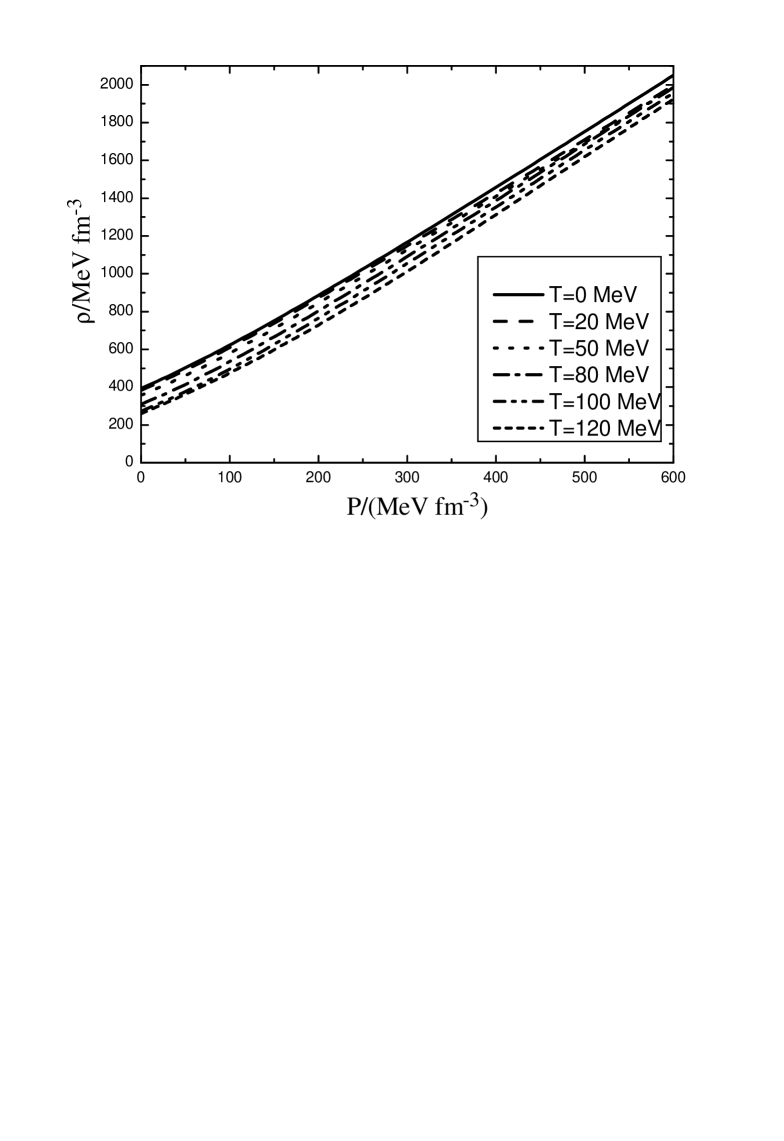
Figure 1: Diagram for the EOS of the strange matter in QMDTD model.

The thermodynamic potential reads

$$Z=-\sum\limits_{i}{T\int_{0}^{\infty}{dk\frac{{dN_{i}(k)}}{{dk}}}}\ln(1+e^{-\beta(\varepsilon_{i}(k)-\mu_{i})}),$$ (7)

where $i$ stands for u, d, s (or $\bar{u},\bar{d},\bar{s}$) quarks, $\mu_{i}$ is the corresponding chemical potential (for anti-quark $\mu_{\bar{i}}=-\mu_{i}$), $\varepsilon_{i}=\sqrt{m_{i}^{2}+k^{2}}$ is the single particle energy and $m_{i}$ is the mass for quarks and anti-quarks. ${{dN_{i}(k)}\mathord{\left/{\vphantom{{dN_{i}(k)}{dk}}}\right.\kern-1.2pt}{dk}}$ is the density of states for various flavour quarks. The density of states of a spherical star has been calculated in ref.s24

$$N_{i}(k)=A_{i}(kR)^{3}+B_{i}(kR)^{2}+C_{i}(kR),$$ (8)

$$A_{i}=\frac{{2g_{i}}}{{9\pi}},$$ (9)

$$B_{i}=\frac{{g_{i}}}{{2\pi}}\{[1+(\frac{{m_{i}}}{k})^{2}]\tan^{-1}(\frac{k}{{m_{i}}})-(\frac{{m_{i}}}{k})-\frac{\pi}{2}\},$$ (10)

$$C_{i} = \frac{{g_{i}}}{{2\pi}}\{\frac{1}{3}+(\frac{k}{{m_{i}}}+\frac{{m_{i}}}{k})\tan^{-1}(\frac{k}{{m_{i}}})-\frac{{\pi k}}{{2m_{i}}}$$ (11)

$$+(\frac{{m_{i}}}{k})^{1.45}\frac{{g_{i}}}{{3.42(\frac{{m_{i}}}{k}-6.5)^{2}+100}}\},$$

where $g_{i}$ is the total degeneracy. For a slowly rotating star, as a zero-th order approximation of the Hartle’s perturbation formalism, we use the density of states of a spherical cavity to calculate.

After getting the thermodynamic potential $Z$, we can derive the energy density $\rho$ and the pressure $p$. The results are s15 s17 -s20

$$p=-\frac{1}{V}\left.{\frac{{\partial(\Omega/n_{B})}}{{\partial(1/n_{B})}}}\right|_{T,\mu_{i}}=-\frac{\Omega}{V}+\frac{{n_{B}}}{V}\left.{\frac{{\partial\Omega}}{{\partial n_{B}}}}\right|_{T,\mu_{i}},$$ (12)

$$\rho=\frac{\Omega}{V}+\sum\limits_{i}{n_{i}\mu_{i}-\frac{T}{V}\left({\frac{{\partial\Omega}}{{\partial T}}}\right)}_{\mu_{i},n_{B}}.$$ (13)

The extra terms in Eqs.(12) and (13) come from the dependence of the quark mass on the baryon density.

The EOS for strange quark star can be calculated from above formula and the result is shown in Fig.1, where the parameters are fixed as $B_{0}=170MeVfm^{-3}$, $m_{s0}=150MeV$ and $T_{c}=170MeV$.

III Uniform rotating strange stars

III.1 Formalism

In this section, we employ Hartle’s formalism to study the slowly rotating strange star. We review this method briefly below and the details can be found in ref.s22 .

The metric of non-rotating configuration is

$$ds^{2}=-e^{\nu(r)}dt^{2}+e^{\lambda(r)}dr^{2}+r^{2}(d\theta^{2}+\sin^{2}\theta d\varphi^{2}).$$ (14)

In hydrostatic equilibrium, $\nu(r)$ and $\lambda(r)$ are determined by the TOV equations

$$\frac{{d\nu}}{{dr}}=-\frac{2}{{\rho+P}}\frac{{dP}}{{dr}},$$ (15)

$$e^{\lambda(r)}=(1-\frac{{2m}}{r})^{-1},$$ (16)

$$\frac{{dm}}{{dr}}=4\pi r^{2}\rho,$$ (17)

$$\frac{{dP}}{{dr}}=\frac{{(P+\rho)(m+4\pi r^{3}P)}}{{r^{2}(1-\frac{{2m}}{r})}},$$ (18)

where $P$ and $\rho$ are the pressure and energy density of strange matter respectively and they relate each other by EOS. The stellar mass $M=m(R)$, where $R$ is the radius of the star and is obtained by solving equation $P(R)=0$. For a slowly rotating star, the configuration is no longer static and spherically symmetric, but axially symmetric instead. The metric becomes

$$ds^{2} = -e^{\nu(r)}(1+2h)dt^{2}+e^{\lambda(r)}[1+\frac{{2\tilde{m}}}{{r-2m}}]dr^{2}$$ (19)

$$+r^{2}(1+2k)[d\theta^{2}+\sin^{2}\theta(d\varphi-\omega dt)^{2}]+O(\omega^{3}),$$

where $\omega(r)$ is the angular velocity of a locally non-rotating inertial frame. Expanding the metric in spherical harmonics, we find

$$\left\{{\begin{array}[]{*{20}c}{h=h(r,\theta)=h_{0}(r)+h_{1}(r)P_{1}(\theta)+h_{2}P(\theta)+...}\\ {\tilde{m}=\tilde{m}(r,\theta)=\tilde{m}_{0}(r)+\tilde{m}_{1}(r)P_{1}(\theta)+\tilde{m}_{2}P(\theta)+...}\\ {k=k(r,\theta)=k_{0}(r)+k_{1}(r)P_{1}(\theta)+k_{2}P(\theta)+...}\\ \end{array}}\right.$$ (20)

It can be proved from symmetric consideration that $h_{1}(r)$, $\tilde{m}_{1}(r)$ and $k_{1}(r)$ vanish. Therefore, under the slow rotation approximation the metric can be written as

$$ds^{2} = -e^{\nu}[1+2(h_{0}+h_{2}P_{2})]dt^{2}+e^{\lambda}[1+\frac{{2(\tilde{m}_{0}+\tilde{m}_{2}P_{2})}}{{r-2m}}]dr^{2}$$ (21)

$$+r^{2}(1+2k_{2}P_{2})[d\theta^{2}+\sin^{2}\theta(dt-\omega d\varphi)^{2}]+O(\omega^{3}),$$

where $e^{\nu}$ and $e^{\lambda}$ can be calculated by TOV equations (15)-(18) and $P_{2}=(3cos\theta-1)/2$.

The rotation not only affects the metric, but also can change the distribution of pressure in the interior of the star. In a co-moving reference frame with the fluid, the pressure correction is

$$P+(P+\rho)p^{*}=P+\Delta P,$$ (22)

and the energy density correction

$$\rho+(P+\rho)\frac{{d\rho}}{{dP}}p^{*}=\rho+\Delta\rho.$$ (23)

Here $p^{*}$ indicates the dimensionless corrections on the pressure. It can also be expanded as

$$p^{*}(r,\theta)=p_{0}^{*}(r)+p_{2}^{*}(r)P_{2}+...$$ (24)

The stress-energy tensor in a rotating star is

$$T^{(0)\nu}_{\mu}+\Delta T^{\nu}_{\mu}=(\rho+\Delta\rho+P+\Delta P)u_{\mu}u^{\nu}+(P+\Delta P)\delta_{\mu}^{\nu},$$ (25)

where

$$\left\{\begin{array}[]{l}u^{t}=(-g_{tt}-2\Omega g_{t\varphi}-g_{\varphi\varphi}\Omega^{2})^{-1/2}\\ u^{\varphi}=\Omega u^{t},u^{r}=u^{\theta}=0\\ \end{array}\right..$$ (26)

$\Omega$ is the angular velocity of fluid observed far from the star. Noting that the perturbed Einstein equation $G^{(0)\nu}_{\mu}+\Delta G^{\nu}_{\mu}=8\pi T^{(0)\nu}_{\mu}+8\pi\Delta T^{\nu}_{\mu}$ and the zeroth order equations $G^{(0)\nu}_{\mu}=8\pi T^{(0)\nu}_{\mu}$, we get

$$\Delta G^{\nu}_{\mu}=8\pi\Delta T^{\nu}_{\mu}.$$ (27)

For the component of $t=\nu$ and $\mu=\phi$ of Eq.(27) , we have

$$\frac{1}{{r^{4}}}\frac{\partial}{{\partial r}}\{r^{4}j(r)\frac{{\partial\varpi}}{{\partial r}}\}+\frac{4}{r}\frac{{dj}}{{dr}}\varpi+\frac{{e^{-(\nu-\lambda)/2}}}{{r^{2}\sin^{3}\theta}}\frac{\partial}{{\partial\theta}}\{\sin^{3}\theta\frac{{\partial\varpi}}{{\partial\theta}}\}$$

$$=\frac{1}{{r^{4}}}\frac{\partial}{{\partial r}}\{r^{4}j(r)\frac{{\partial\Omega}}{{\partial r}}\}+\frac{{e^{-(\nu-\lambda)/2}}}{{r^{2}\sin^{3}\theta}}\frac{\partial}{{\partial\theta}}\{\sin^{3}\theta\frac{{\partial\Omega}}{{\partial\theta}}\},$$ (28)

where

$$j(r)=e^{-(\nu+\lambda)/2}$$ (29)

and we have defined $\varpi=\Omega-\omega$. For the uniform rotation, the angular velocity of fluid is a constant $\Omega=const.$. Therefore, the right hand side of Eq.(III.1) vanishes. We expand $\varpi(r,\theta)$ s25 :

$$\varpi(r,\theta)=\sum\limits_{l=1}^{\infty}{\varpi_{l}(r)(-\frac{1}{{\sin\theta}}\frac{{dP_{l}}}{{d\theta}})}.$$ (30)

Then the radial function of ${\varpi_{l}(r)}$ satisfies

$$\frac{1}{{r^{4}}}\frac{d}{{dr}}\{r^{4}j(r)\frac{{d\varpi_{l}}}{{dr}}\}+\{\frac{4}{r}\frac{{dj}}{{dr}}-e^{-(\nu-\lambda)/2}\frac{{l(l+1)-2}}{{r^{2}}}\}\varpi_{l}=0.$$ (31)

At large $r$, ${\varpi_{l}(r)}$ has the form

$$\varpi_{l}(r)\to const.r^{-l-2}+const.r^{l-1}.$$ (32)

At infinity where the spacetime is flat, $\omega$ must decrease faster than $1/r^{3}$. Because of $\varpi=\Omega-\omega$, only the coefficient of $l=1$ in the $\varpi$ expansion does not vanish and Eq.(31) reduces to

$$\frac{1}{{r^{4}}}\frac{d}{{dr}}\{r^{4}j(r)\frac{{d\varpi}}{{dr}}\}+\frac{4}{r}\frac{{dj}}{{dr}}\varpi=0,$$ (33)

where $\varpi=\varpi_{1}(r)$. Outside the star $j(r)=1$, the solution reads

$$\varpi(r)=\Omega-\frac{{2J}}{{r^{3}}},$$ (34)

where the constant $J$ is identified as the total angular momentum of star and satisfies

$$J=\int{T_{\varphi}^{t}\sqrt{-{}^{3}g}}dV,$$ (35)

where ${}^{3}g$ is the determinant of metric of space components. The moment of inertia is simply

$$I={\raise 3.01385pt\hbox{$J$}\!\mathord{\left/{\vphantom{J\Omega}}\right.\kern-1.2pt}\!\lower 3.01385pt\hbox{$\Omega$}}.$$ (36)

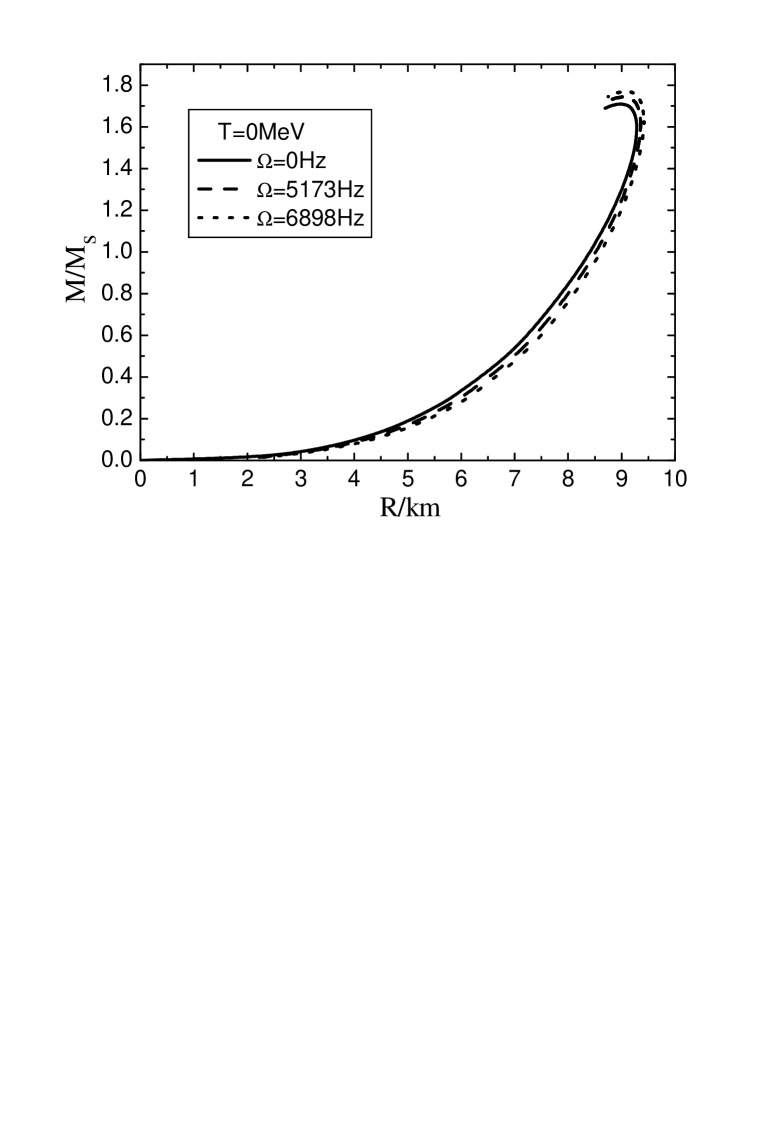
Figure 2: The radius $R$ in km vs. mass $M/M_{s}$ at the temperature $T=0MeV$ for different angular velocity $\Omega$.

Figure 3: The radius $R$ in km vs. mass $M/M_{s}$ at the temperature $T=50MeV$ for different angular velocity $\Omega$.

The components $\nu=\mu=t$ and $\nu=\mu=r$ of Eq.(27) and the terms $l=0$ in the expansion (20) lead to

$$\frac{{d\tilde{m}_{0}}}{{dr}}=4\pi r^{2}p_{0}^{*}(\rho+P)\frac{{d\rho}}{{dP}}+\frac{1}{{12}}j^{2}r^{4}\left({\frac{{d\omega}}{{dr}}}\right)^{2}-\frac{1}{3}r^{3}\frac{{dj^{2}}}{{dr}}\varpi^{2},$$ (37)

$$\frac{{dh_{0}}}{{dr}}-\frac{{\tilde{m}_{0}r^{2}}}{{(r-2m)^{2}}}(8\pi P+\frac{1}{{r^{2}}})=\frac{{4\pi(\rho+P)r^{2}}}{{r-2m}}p_{0}^{*}-\frac{1}{{12}}\frac{{r^{2}}}{{r-2m}}j^{2}\left({\frac{{d\omega}}{{dr}}}\right)^{2}.$$ (38)

Another constraint between the perturbations of the metric and those of energy and pressure comes from the hydrostatic equilibrium, i.e. the conservation of stress-energy tensor of perfect fluid $T^{\mu\nu}_{;\nu}=0$. In the non-rotating case, it can be expressed as

$$\frac{{p_{,i}}}{{p+\rho}}-\frac{{\nu_{,i}}}{{2\nu}}=0$$ (39)

and in the rotating case, the corresponding perturbation equation reads

$$p^{*}_{,i}+h_{,i}-\frac{1}{2}(e^{-\nu}\varpi^{2}r^{2}\sin^{2}\theta)_{,i}=0.$$ (40)

For the terms $l=0$, we find

$$\frac{{dp_{0}^{*}}}{{dr}}+\frac{{dh_{0}}}{{dr}}-\frac{1}{3}\frac{d}{{dr}}(e^{-\nu}\varpi^{2}r)=0.$$ (41)

Combining Eqs.(41) and (38), we find

$$-\frac{{dp_{0}^{*}}}{{dr}}+\frac{1}{{12}}\frac{{r^{2}}}{{r-2m}}j^{2}\left({\frac{{d\omega}}{{dr}}}\right)^{2}+\frac{1}{3}\frac{d}{{dr}}(\frac{{r^{3}j^{2}\varpi^{2}}}{{r-2m}})$$

$$=\frac{{4\pi(\rho+P)r^{2}}}{{r-2m}}p_{0}^{*}+\frac{{\tilde{m}_{0}r^{2}}}{{(r-2m)^{2}}}(8\pi P+\frac{1}{{r^{2}}}).$$ (42)

On the other hand, one can prove that the increasing of stellar mass $\delta M$ and mean radius $\delta R$ are given by s22

$$\delta M=\tilde{m}_{0}(R)+\frac{{J^{2}}}{{R^{3}}},$$ (43)

$$\delta R=p_{0}^{*}(P+\rho)/\left({\frac{{dP}}{{dr}}}\right).$$ (44)

When EOS, $\Omega$ and the boundary value of $P(0)$ are given, we can integrate the TOV equations until reaching the surface of the star $P(R)=0$. Then we solve the Eq.(33), Eq.(37) and Eq.(III.1) to get the perturbations and finally calculate the moment of inertia by Eq.(36), the correction of the mass and radius in rotational case by Eq.(43) and Eq.(44). We do this numerical calculation with the rotational frequencies smaller than the Keplerian frequency

$$\Omega^{2}<\Omega_{k}^{2}\sim M/R^{3},$$ (45)

which is required by the Hartle’s methods22 .

III.2 Results

III.2.1 M-R curves

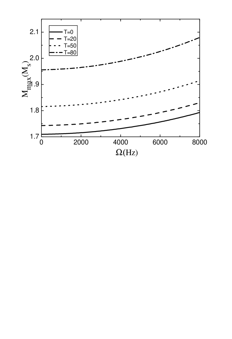
Figure 4: The increase of maximum mass $\delta M_{max}/M_{s}$ vs. the angular velocity $\Omega$ at different temperatures.

The Mass-Radius relation is one of the main results which distinguishes the strange stars and the neutron stars. In our calculation, the M-R relations not only depend on temperature $T$, but also on angular velocity $\Omega$. Fix the temperature $T=0$ and $50MeV$, the M-R curves for different $\Omega$ are shown in Fig.2 and 3, respectively. By using Fig.2, Fig.3 and Eq.(45), we find Keplerian frequency $\Omega_{k}\approx 1.5\times 10^{4}Hz$, which is much larger than the frequencies used in Fig.2 and Fig.3. It is seen that the maximum mass and the corresponding radius increase with $\Omega$. To show the temperature effect more transparently, we plot the $M_{max}$ vs. $\Omega$ curves for different temperatures in Fig.4, and see that for a fixed $\Omega$, $M_{max}$ increases with temperature. The effect of rotation becomes more and more important when temperature increases. From Fig.4, we can express the increase of the maximum mass by a simple formula

$${\raise 3.01385pt\hbox{${\delta M_{\max}}$}\!\mathord{\left/{\vphantom{{\delta M_{\max}}{M_{s}}}}\right.\kern-1.2pt}\!\lower 3.01385pt\hbox{${M_{s}}$}}\propto\Omega^{2},$$ (46)

where $M_{s}$ is the mass of the sun. This is very reasonable because all perturbations in Hartle’s method are assumed to be proportional to the square of the angular velocity of the fluid.

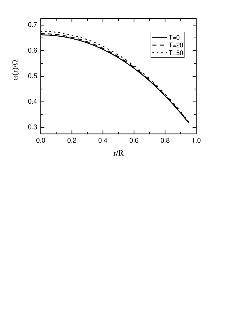
Figure 5: The ratio of angular velocity of inertial frame and fluid in the interior of the star $\omega(r)/\Omega$ vs. $r/R$, where $R$ is the radius of the star, at the temperatures $T=20,50MeV$.

III.2.2 The effect of frame dragging

The frame dragging is a general relativistic effect for a rotating object. To show the effect of frame dragging in a slowly rotating star, we plot the $\omega(r)/\Omega$ vs. $r/R$ curves for different temperatures in Fig.5. We see from Fig.5 that this effect decreases when one approaches to the surface of star, and the dragging increases when temperature increases.

Figure 6: The moment of inertia $I_{45}$ vs. mass $M/M_{s}$ at the different temperatures $T=0,20,50,80MeV$ for the star rotating at the frequency $\Omega=200Hz$.

III.2.3 The moment of inertia

Besides the M-R relation, much information for the configuration of a strange star is provided by its moment of inertia, which is one of the essential facts to understand many observational phenomenons. Fig.6 shows the relation of the moment of inertia-Mass. We see that the moment of inertia will increase with temperature.

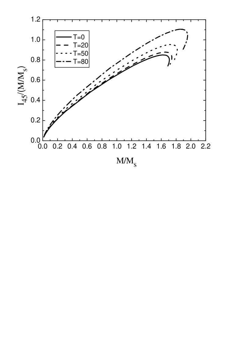
Figure 7: The ratio of the moment of inertia and the stellar mass $I_{45}/(M/M_{s})$ vs. mass $M/M_{s}$ at the different temperatures $T=0,20,50,80MeV$.

III.2.4 Horizontal-branch oscillation

Recently Stella and Vietris30 made a link between quasi-periodic oscillations(QPO) and general relativistic Lense-Thirring precession caused by frame dragging. The low frequency of QPO, called horizontal-branch oscillations(HBO), is the frequency of the L-T precession of an inclined circular orbit with Keplerian orbital frequency. Psaltis et al.s31 found that the ratios of the moments of inertia and masses ${{I_{45}}\mathord{\left/{\vphantom{{I_{45}}{(\frac{M}{{M_{s}}})}}}\right.\kern-1.2pt}{(\frac{M}{{M_{s}}})}}$ of five bright sources (GX 17+2, Cyg X-2, GX 5-1, Sco X-1, GX 340+0) satisfy $I_{45}/(M/M_{s})>2.3$. Kalogera and Psaltiss32 calculate this ratio for various models of neutron star and argue that this requirement cannot be satisfied for neutron stars.

Here we suppose these five sources are strange stars and discuss whether the condition about $I_{45}/(M/M_{s})$ is satisfied. Fig.7 tells us that to satisfy the condition $I_{45}/(M/M_{s})>2.3$ one require too high temperature which is over $120MeV$ from the Figure. This makes the validity of the suggestion by Stella and Vietri to be challenged also for the strange stars.

IV Differential Rotation Strange Stars

We will study the configuration of differential rotating star, i.e. the angular velocity of the fluid $\Omega=\Omega(r,\theta)$, in this section. Obviously, differential rotation will affect the evolution of a hot and new-born star. Noting that Hartle’s method can only be used to study the uniform rotational star, an extension is needed when star is newly born and differentially rotating.

IV.1 Formulism

It can easily be seen that the Eq.(III.1) is still valid in the case of differential rotation, but the right hand side does not varnish now. Expanding $\Omega(r,\theta)$ (and then $\varpi(r,\theta)$) by the Legendre functions

$$\Omega(r,\theta)=\sum\limits_{l=1}^{\infty}{\Omega_{l}(r)(-\frac{1}{{\sin\theta}}\frac{{dP_{l}}}{{d\theta}})}.$$ (47)

Eq.(III.1) becomes

$$\frac{1}{{r^{4}}}\frac{d}{{dr}}\{r^{4}j(r)\frac{{d\varpi_{l}}}{{dr}}\}+\{\frac{4}{r}\frac{{dj}}{{dr}}-e^{-(\nu-\lambda)/2}\frac{{l(l+1)-2}}{{r^{2}}}\}\varpi_{l}$$

$$=\frac{1}{{r^{4}}}\frac{d}{{dr}}\{r^{4}j(r)\frac{{d\Omega_{l}}}{{dr}}\}-e^{-(\nu-\lambda)/2}\frac{{l(l+1)-2}}{{r^{2}}}\Omega_{l}.$$ (48)

Remember that outside the star, there is no fluid, $\Omega_{l}(r)=0$, therefore, $\varpi_{l}(r)$ in Eq.(IV.1) still has the form

$$\varpi_{l}(r)\to const.r^{-l-2}+const.r^{l-1}.$$

A similar discussion can be made as that of the uniform rotation case: $\omega$ should decrease faster than $1/r^{3}$ if the spacetime is asymptotically flat. As a result, only the term with $l=1$ remains, while $\varpi=\varpi_{1}(r)$ and $\Omega=\Omega_{1}(r)$ are the functions of radial coordinate only. Eq.(IV.1) is simplified to be

$$\frac{1}{{r^{4}}}\frac{d}{{dr}}\{r^{4}j(r)\frac{{d\varpi}}{{dr}}\}+\frac{4}{r}\frac{{dj}}{{dr}}\varpi=\frac{1}{{r^{4}}}\frac{d}{{dr}}\{r^{4}j(r)\frac{{d\Omega}}{{dr}}\},$$ (49)

with $\varpi^{\prime}(0)=\Omega^{\prime}(0)$. The solution is

$$\varpi(r)=const.-\frac{{2J}}{{r^{3}}}.$$ (50)

Here the constant $J$ can still be interpreted as the total angular momentum of the star. We obtain

$$\varpi(R)=\Omega(R)-\frac{{2J}}{{R^{3}}}$$ (51)

at the surface of star $r=R$. In differential rotation, the angular velocity of fluid depends on the radial coordinate. This means that in the internal regime of the star, a very thin layer $r\to r+dr$ of the fluid rotates with the same angular velocity $\Omega(r)$ and generates angular momentum of this layer $dJ$, which satisfies,

$$dJ=\Omega(r)dI.$$

$dI$ is the moment of inertia of this thin layer. Hence the total moment of inertia of the star is

$$I=\int{dI=\int{dJ/\Omega=\int{({{T_{\varphi}^{t}}\mathord{\left/{\vphantom{{T_{\varphi}^{t}}\Omega}}\right.\kern-1.2pt}\Omega})\sqrt{-{}^{3}g}dV}}},$$ (52)

where the Eq.(35) is used at the last equality. Since the differential rotation changes the derivatives of stress-energy tensor in hydrostatic equilibrium, we find

$$\frac{{p_{,i}}}{{p+\rho}}-\frac{{u_{,i}^{t}}}{{u^{t}}}+F(\Omega)\Omega_{,i}=0,$$ (53)

where

$$F(\Omega)=-\frac{{g_{t\phi}+\Omega g_{\phi\phi}}}{{g_{tt}+2\Omega g_{t\phi}+\Omega^{2}g_{\phi\phi}}}.$$ (54)

In the slowly rotating approximation, the effect of differential rotation is considered as perturbation. Therefore we have

$$p_{,i}^{*}+h_{,i}-\frac{1}{2}(\varpi^{2}r^{2}\sin^{2}\theta e^{-\nu})_{,i}+(e^{-\nu}\varpi r^{2}\sin^{2}\theta)\Omega_{,i}=0.$$ (55)

For the term $l=0$ and $i=r$, Eq.(55) gives

$$p_{0,r}^{*}+h_{0,r}-\frac{1}{3}(\varpi^{2}r^{2}e^{-\nu})_{,r}+\frac{2}{3}(e^{-\nu}\varpi r^{2})\Omega_{,r}=0.$$ (56)

Combining with Eq.(38), we find

$$-\frac{{dp_{0}^{*}}}{{dr}} = \frac{{4\pi(\rho+p)}}{{r-2m}}r^{2}p_{0}^{*}+\frac{{\tilde{m}_{0}(8\pi pr^{2}+1)}}{{(r-2m)}}-\frac{{r^{4}j^{2}}}{{12(r-2m)}}(\frac{{d\omega}}{{dr}})^{2}$$ (57)

$$-\frac{1}{3}\frac{d}{{dr}}(\frac{{r^{3}j^{2}\varpi^{2}}}{{r-2m}})+\frac{2}{3}\frac{{r^{3}j^{2}\varpi}}{{r-2m}}\frac{{d\Omega}}{{dr}},$$

with boundary conditions $\tilde{m}_{0}=p^{*}_{0}=0$. Eq.(37) is valid in the differential rotation, because the derivatives of that $\Omega(r)$ do not appear in both of the right and left hand sides of Eq.(27) as in the uniform rotation. We can solve Eq.(37)(57)numerically.

Figure 8: The radius $R$ vs. mass $M/M_{s}$ at the temperature $T=0MeV$ for the different values of $\beta$.

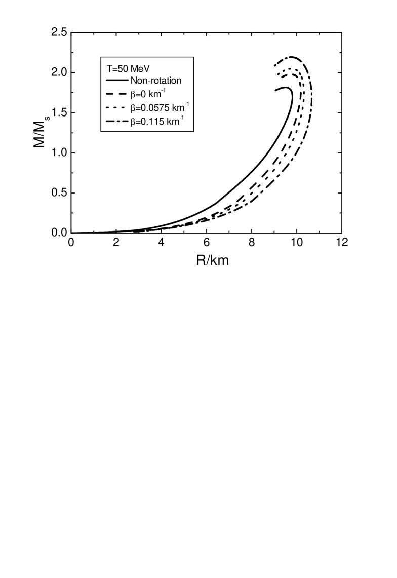
Figure 9: The radius $R$ vs. mass $M/M_{s}$ at the temperature $T=50MeV$ for the different values of $\beta$.

IV.2 Results

We employ the distribution of the angular velocity of the fluid

$$\Omega(r)=\Omega_{c}e^{-\beta r},$$ (58)

where $\Omega_{c}$ is the angular velocity of the core and $\beta$ is a constant, to investigate the influences of differential rotation. Fixing the surface angular velocity $\Omega_{e}=10346Hz$, which is still smaller than the Mass-shedding limit at the surface of a uniformly rotating star and satisfies the slowly rotating approximation, we show the M-R curves for $\Omega(r)$ at temperature $T=0$ and $50MeV$ in Fig.8 and Fig.9 respectively. We see that the effect of $\beta$ on $M_{max}$ is remarkable, and the result reduces to the uniform rotation when $\beta=0$. A differentially rotating strange star can sustain more mass than that of the uniform rotating configuration. The curves of the maximum mass increase $\delta M_{max}/M_{max}$ vs. $\Omega_{c}/\Omega_{e}$, the ratio of the angular velocity at the core and at the surface, are shown in Fig.10. We see that $\delta M_{max}/M_{max}$ changes considerably with temperature and $\Omega_{c}/\Omega_{e}$. A hot and differentially rotating strange star will suffer more maximum mass increase.

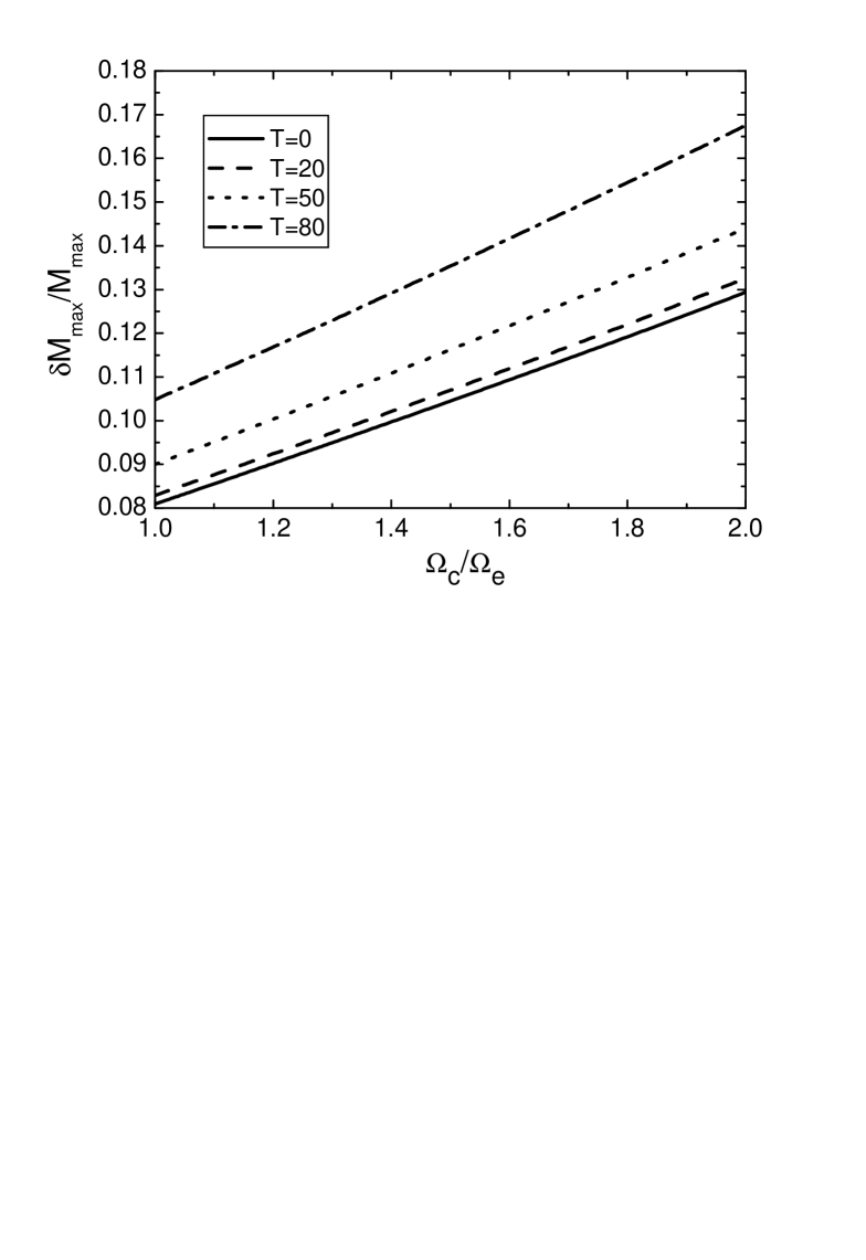
Figure 10: The ratio of the maximum mass increase $\delta M_{max}/M_{max}$ vs. $\Omega_{c}/\Omega_{e}$, the ratio of the angular velocity at the core and at the surface at the different temperatures $T=0,20,50,80MeV$.

Similarly, we can address the effect of $\Omega(r)$ on the moment of inertia at temperature $T=0$ and $50MeV$. We show this effect in Fig.11 and Fig.12 respectively. Comparing to Fig.8 and Fig.9, we find that corresponding to the mass, the effect of $\beta$ on the moment of inertia is small. This is reasonable and expected, because in the slowly rotating approximation, the effect of rotation is too weak to change the star’s shape (almost spherical), which has strong influence on the moment of inertia.

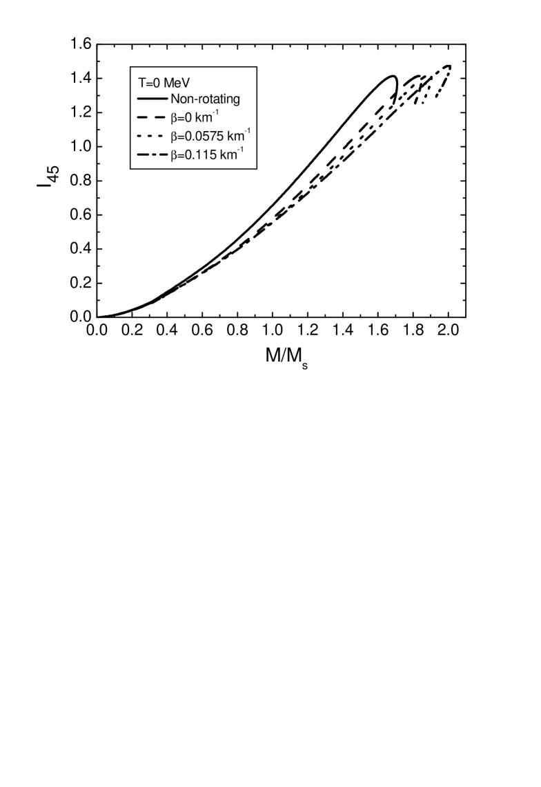
Figure 11: The moment of inertia $I_{45}$ vs. mass $M/M_{s}$ at the temperature $T=0MeV$ for the different values of $\beta$.

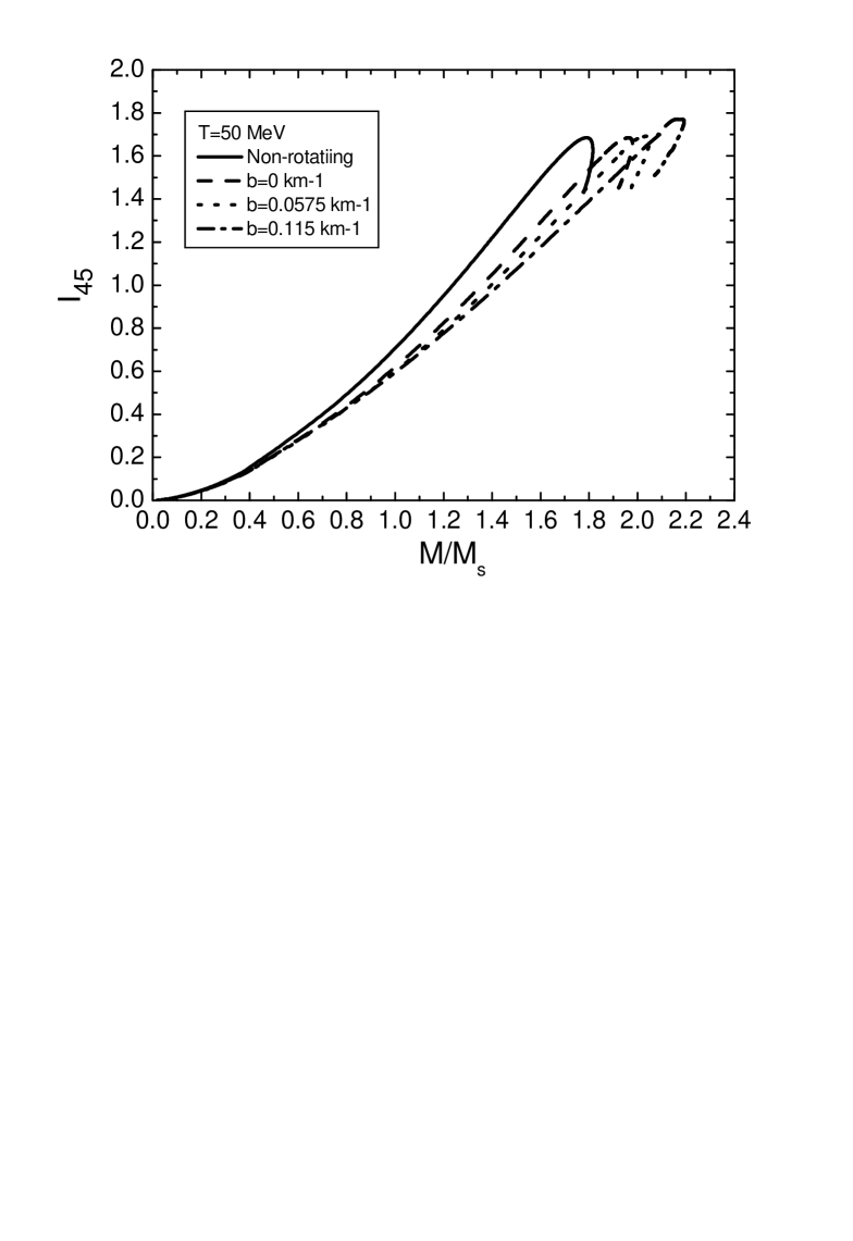
Figure 12: he moment of inertia $I_{45}$ vs. mass $M/M_{s}$ at the temperature $T=50MeV$ for the different values of $\beta$.

V Conclusion and Discussion

As shown by Gupta et. al.s22 , the parameters of the EOS in the QMDTD model have few influences on the configuration of the strange star. We extend their work to the rotational case and have studied the slowly rotating strange star with uniform angular velocity, employing the QMDTD model and the Hartle’s method. The M-R relation , the moment of inertia and the frame dragging of strange star with different rotating frequencies are given. We found that mass, the moment of inertia and the frame dragging increase when temperature increases. We also found that the challenges of Stella and Vietri for HBO and the moment of inertia $I_{45}/(M/M_{s}>2.3)$ for five bright sources being neutron stars also exist for the strange star. We cannot use the strange star to solve this difficulty.

Furthermore, we have extended the Hartle’s method to study the differential rotating strange star with $\Omega=\Omega(r)$. We found that the massive strange star can be prepared in the differential rotation. In the slowly rotating approximation, compared to the temperature the differential rotation has less effect on changing the moment of inertia of the star.

- (1) C. Alcock, E. Farhi and A. Olinto, ApJ 310 (1986) 261.
- (2) P. Haensel, J. L. Zdunik and R. Schaefer, A&A 160 (1986) 121.
- (3) K. S. Cheng, Z. G. Dai, D. M. Wai and T. Lu, Science 280 (1998) 407.
- (4) I. Bombaci, Phys. Rev. C55 (1997) 1587.
- (5) X. D. Li, I. Bombaci, M. Dey, J. Dey and E. P. J. van den Heuvel, Phys. Rev. Lett. 83 (1999) 3776.
- (6) B. Link, R. I. Epstein and J. M. Lattimer, Phys. Rev. Lett. 83 (1999) 3362.
- (7) M. Prakash, I. Bombaci, P.J. Ellis, J.M. Lattimer and R. Knorren, Phys. Rep. 280 (1997) 1.
- (8) Z. G. Dai, Q. H. Peng and T. Lu, ApJ 440 (1995) 815.
- (9) M. Dey, I. Bombaci, J. Dey, S. Ray and B. C. Samanta, Phys. Lett. B 438 (1998) 123.
- (10) J. D. Anand, N. Chandrika Devi, V. K. Gupta and S. Singh, ApJ 538 (2000) 870.
- (11) S. Singh, N. Chandrika Devi, V. K. Gupta, Asha Gupta and J. D. Anand, J. Phys. G28 (2002) 2525.
- (12) G. N. Fowler, S. Raha and R. M. Weiner, Z. Phys. C9 (1981) 271.
- (13) S. Chakrabarty, Phys. Rev. D43 (1991) 627, Phys. Rev. D48 (1993) 1409.
- (14) G. Lugones and O. G. Benrenuto, Phys. Rev. D52 (1995) 1276, Phys. Rev. D51 (1995) 1989.
- (15) G. X. Peng, H. C. Chiang, B. S. Zou, P. Z. Ning and S. J. Luo, Phys. Rev. C62 (2000) 025801.
- (16) P. Wang, Phys. Rev. C62 (2000) 015204.
- (17) Y. Zhang and R. K. Su, Phys. Rev. C65 (2002) 035202.
- (18) Y. Zhang and R. K. Su, Phys. Rev. C67 (2003) 015202.
- (19) Y. Zhang, R. K. Su, S. Ying and P. Wang, Europhys. Lett. 56 (2001) 361.
- (20) Y. Zhang and R. K. Su J. Phys. G30 (2004) 811.
- (21) V. K. Gupta, A. Gupta, S. Sigh and J. D. Anand, Int. J. Mod. Phys. D12 (2003) 583.
- (22) J. B. Hartle, ApJ 150 (1967) 1005, J. B. Hartle and K. S. Thorne, ApJ 153 (1968) 807.
- (23) T. D. Lee, Particle Physics and Introduction to Field Theory Harwood Academic, Chur (1981).
- (24) Y. Zhang, W. L. Qian, S. Q. Ying and R. K. Su, J. Phys. G27 (2001) 2241.
- (25) T. Regge and J. Wheeler, Phys. Rev. 108 (1957) 1063.
- (26) M. Bejger and P. Haensel, A&A 396 (2003) 917.
- (27) S. L. Stella and M. Vietri, Nucl. Phys. B69 (1998) 135.
- (28) D. Psaltis, R. Wijnands, J. Homan, P. G. Jonker, Mi. van der Klis, M. C. Miller, F. K. Lamb, E. Kuulkers, Jan van Paradijs and W. H. G. Lewin , ApJ 520 (1999) 763.
- (29) V. Kalogera and D. Psaltis, Phys. Rev. D108 (1957) 1063.