Binary black hole initial data from matched asymptotic expansions

Abstract

We present an approximate metric for a binary black hole spacetime to construct initial data for numerical relativity. This metric is obtained by asymptotically matching a post-Newtonian metric for a binary system to a perturbed Schwarzschild metric for each hole. In the inner zone near each hole, the metric is given by the Schwarzschild solution plus a quadrupolar perturbation corresponding to an external tidal gravitational field. In the near zone, well outside each black hole but less than a reduced wavelength from the center of mass of the binary, the metric is given by a post-Newtonian expansion including the lowest-order deviations from flat spacetime. When the near zone overlaps each inner zone in a buffer zone, the post-Newtonian and perturbed Schwarzschild metrics can be asymptotically matched to each other. By demanding matching (over a $4$-volume in the buffer zone) rather than patching (choosing a particular $2$-surface in the buffer zone), we guarantee that the errors are small in all zones. The resulting piecewise metric is made formally $C^{\infty}$ with smooth transition functions so as to obtain the finite extrinsic curvature of a $3$-slice. In addition to the metric and extrinsic curvature, we present explicit results for the lapse and the shift, which can be used as initial data for numerical simulations. This initial data is not accurate all the way to the asymptotically flat ends inside each hole, and therefore must be used with evolution codes which employ black hole excision rather than puncture methods. This paper lays the foundations of a method that can be straightforwardly iterated to obtain initial data to higher perturbative order.

I Introduction

The simulation of binary black-hole systems is of fundamental physical interest as the purely general relativistic two-body problem. It is also of astrophysical interest, since accurate simulations of the late inspiral and merger phases of such binaries will considerably help the effort to detect the gravitational-wave signals and extract information from them Baumgarte and Shapiro (2003). Simulation reduces to the numerical solution of the Cauchy problem: take some initial data and evolve it. The evolution is difficult for many reasons, although in recent years there has been much progress. Still, any evolution is only as good as its initial data.

A key issue of initial data is astrophysical realism. The goal is to compute data on a hypersurface that represents one moment in time of an astrophysical inspiral of two black holes. If such an inspiral is defined by initial conditions in the distant past for widely separated black holes, then the only way to obtain the exact data at a later time would be to perform the actual evolution using the full Einstein equations. This procedure, however, is computationally expensive and thus impractical. On the other hand, several schemes have been developed to pose initial data that approximates the astrophysical situation at a given time. These schemes are typically either based on post-Newtonian (PN) methods or on the numerical solution of the constraint equations of relativity.

For example, the literature provides many types of initial data for black holes in approximately circular orbits Cook (1994); Matzner et al. (1999); Baumgarte (2000); Marronetti and Matzner (2000); Cook (2000); Grandclément et al. (2002); Pfeiffer et al. (2002); Baker (2002); Tichy et al. (2003a, b); Tichy and Brügmann (2004); Yo et al. (2004); Cook and Pfeiffer (2004) that satisfy the constraints of the Einstein equations. To obtain such data, certain assumptions are made, such as conformal flatness and quasi-circularity. These assumptions are expected to be good approximations within a certain error, although the astrophysical metric after a long inspiral is known to be not exactly conformally flat and the orbit not perfectly circular.

In this paper we consider a post-Newtonian method combined with black hole perturbation theory to construct approximate inspiral initial data. For large to intermediate separations of compact objects, an astrophysically relevant approximate spacetime can be obtained far from the black holes by analytical post-Newtonian and post-Minkowskian methods Blanchet (2006). One advantage of such methods is that they allow systematic improvements through higher order expansions (compared to numerical constraint solving schemes which typically include only the correct lowest order PN behavior). In their regime of validity, PN methods do result in appropriate deviations from conformal flatness and in non-circular inspiral orbits. The main disadvantage of PN methods is that, by construction, they are generally believed to fail in the final phase of the inspiral for fast moving objects, and also close to non-pointlike objects with horizons. On the other hand, black hole perturbation theory provides an accurate spacetime in a region of the manifold sufficiently close to the background black hole. The main disadvantage of this theory is that it fails sufficiently far from the background hole and, thus, cannot provide information about the dynamics of the entire spacetime.

In what follows, we take a concrete step toward combining PN theory with black hole perturbation theory using the mathematical machinery of asymptotic matching. The method maintains the potential for systematic improvement through higher order expansions, although we only work at low order here Yunes and Tichy (2006a); Yunes and Tichy (2006b). From the PN approach the method inherits its astrophysical justification, i.e. that for sufficient separation between the holes the method will yield metric components that are correct up to uncontrolled remainders of certain orders. The uncontrolled remainders in the metric components have different effects on different quantities, and it is of interest to see how other quantities such as the binding energy compare to those of other initial data sets in the literature. This question is beyond the scope of this article, but should be addressed in the future.

Concretely, we have to discuss how black holes are incorporated in our approach. While formally PN methods assume slow motion and weak internal gravity of the sources, it has been shown that the results hold as well for objects such as black holes with strong internal gravity Thorne and Hartle (1985) as long as one is not too close to these objects. Near each black hole, a tidally perturbed Schwarzschild or Kerr spacetime provides another analytical approximation. Given that different approximate metrics can be constructed from different scale expansions, it is natural to try the method of matched asymptotic expansions Bender and Orszag (1999). If there is an overlap region (also known as a buffer zone) where both approximations (post-Newtonian and tidal perturbation) are valid, a diffeomorphism can be constructed between charts used in different regions of the manifold by different approximation schemes. Matching—demanding that both approximation schemes have the same asymptotic form in the overlap region—relates physical observables in the different regions, i.e. ensures that both expansions represent the same physical system.

The first attempt to construct initial data in such a way was by Alvi Alvi (2000). By construction, there are discontinuities in the data, which were found to be too large for numerical experiments Jansen and Brügmann (2002). Alvi’s fundamental problem was that, in the terminology of textbooks such as Bender’s Bender and Orszag (1999), he did not match (construct expansions asymptotic to each other everywhere in the overlap region) but rather patched (set approximate solutions to the Einstein equations equal to each other on specified 2-surfaces) so that large errors in the extrinsic curvature were possible. Alvi’s Table I shows that his spatial metric near the black holes is discontinuous apart from the Minkowski terms (independent of $G$) in either region. Such discontinuities are problematic for numerical relativity, since part of the initial data is the extrinsic curvature which includes derivatives of the spacetime metric. Smoothing can be attempted, for example with transition functions as in Alvi’s next paper Alvi (2003), but it is not trivial to implement—especially with such large discontinuities—without adding unphysical content to the initial data. There is also the issue of making sure that the initial data slicing is treated consistently in the various expansions, which Alvi addressed to some extent but did not always make explicit his assumptions. Finally, there was a problem with the accuracy to which Alvi calculated metric components. Construction of the extrinsic curvature requires terms in the expansions that Alvi did not calculate because he assumed (incorrectly) that the counting of orders follows the standard pattern used in deriving post-Newtonian equations of motion.

The main point of this paper is that we are able to correct the mathematical problems with Alvi’s approach, and that we provide initial data for actual numerical evolutions. We use true asymptotic matching to construct a piecewise metric for two black holes in circular orbit, including terms of order the gravitational constant $G$ on the diagonal of the metric and $O(G)^{3/2}$ off the diagonal. We then remove the piecewise nature of the approximate metric by “merging” or “smoothing” the solutions in the buffer zones, thus generating a uniform approximate metric. We do this by constructing smooth transition functions so that the uniform approximate solution is in principle $C^{\infty}$, although in practice higher-order derivatives will be less accurate than lower-order ones. These transition functions are carefully constructed to avoid introducing errors in the smoothed global metric larger than those already contained in the approximate solutions. This metric allows for the calculation of the lapse to $O(G)$, the shift to $O(G)^{3/2}$, and the extrinsic curvature to $O(G)^{3/2}$. Although this data contains only the first order deviations from flat spacetime, our approach does include the tidal perturbations near the black holes. Strictly speaking, these tidal perturbations are valid only near the horizons—our approach cannot model the asymptotically flat ends inside the holes and therefore must be used in numerical evolutions with excision rather than punctures. Our formalism can be extended to higher order by including more precise post-Newtonian Blanchet et al. (2004) and black hole perturbation theory results Poisson (2005) already in the literature.

By construction, our initial data satisfies the constraints only up to uncontrolled remainders of a certain order. Therefore, this data may still need to be projected to the constraint hypersurface via a conformal decomposition. One avenue worth exploring is that since the constraint violations are $O(G)^{3/2}$ or smaller, it may be possible to find a constraint projection algorithm that changes the physical content of our initial data only at a comparably small order. In this manner, the formalism presented here can potentially be used to construct extremely accurate background data for constraint solving. This hybrid combination of an accurate background $4$-metric plus constraint solving might potentially lead to very astrophysically realistic initial data, which then could be compared and tested against other sets already in the literature.

This paper is organized as follows: Sec. II describes the method of asymptotic matching as applicable to this problem. Sec. III discusses the near zone expansion of the metric and determines its asymptotic expansion in the overlap region. Sec. IV concentrates on the inner zone expansion of the metric and expands it asymptotically in the overlap region. Sec. V applies asymptotic matching to the metrics to obtain matching relations between expansion coefficients and a map that relates the charts used in the different regions. Sec. VI constructs the global metric, discusses its properties, and builds transition functions to eliminate discontinuities between local approximations. Sec. VII computes the extrinsic curvature, lapse and shift. Sec. VIII concludes and points toward future research.

Throughout this paper we use geometrized units ($G=c=1$) and we have relied heavily on symbolic manipulation software, such as MAPLE and MATHEMATICA. We use the tilde as a relational symbol such that $a\sim b$ means “$a$ is asymptotic to $b$” Bender and Orszag (1999). When we refer to our results as “global,” we mean that they cover the region of most interest to numerical relativity. Strictly speaking, our results do not cover the radiation zone (further from the binary than a reduced wavelength) or the asymptotically flat ends inside the holes. However, obtaining the radiation-zone solution and matching it to the near-zone solution is a solved problem Blanchet (2006) and the asymptotic ends inside the holes can be removed with excision before numerically evolving the initial data.

II Approximation Regions and Precision

Let us now consider a binary black hole spacetime, with holes of mass $m_{1}$ and $m_{2}$, total mass $m=m_{1}+m_{2}$ and spatial coordinate separation $b$. The manifold (Fig. 1) can be divided into $4$ submanifolds, the boundaries of which cannot be determined precisely due to the presence of uncontrolled remainders in black hole perturbation theory (BHPT) and post-Newtonian (PN) asymptotic series. Nonetheless, an approximate subdivision is possible and we make one as follows:

1. The inner zone of Black Hole $1$, (submanifold ${\cal{C}}_{1}$): $R_{1}\ll b$, where $R_{A}$ is the distance from the $A$th black hole in isotropic coordinates. In this region, the metric is obtained via black hole perturbation theory as an expansion in $\epsilon_{(1)}=R_{1}/b$. Alvi (2000); Thorne and Hartle (1985).

2. The inner zone of Black hole $2$, (submanifold ${\cal{C}}_{2}$): $R_{2}\ll b$, where the metric is obtained in the same manner as in region ${\cal{C}}_{1}$ but with labels 1 and 2 swapped.

3. The near zone, (submanifold ${\cal{C}}_{3}$): $r_{A}\gg m_{A}$ and $r\leq\lambda/2\pi$, where $\lambda$ is the wavelength of gravitational radiation, $r$ is the distance from the binary center of mass in harmonic coordinates, and $r_{A}-m_{A}$ is the separation in harmonic coordinates from the horizon of the $A$th black hole. In this region, a post-Newtonian approximation is used for the metric with an expansion parameter $\epsilon_{(3)}=m_{A}/r_{A}$ Blanchet (2006) which is formally treated as the same order for both values of $A$.

4. The far zone, (submanifold ${\cal{C}}_{4}$): $r\geq\lambda/2\pi$, where the metric is obtained from a post-Minkowski calculation Will and Wiseman (1996).

These zones are shown schematically in Fig. 1, projected onto the orbital plane. In these figures, the near zone is shown in dark gray, the inner zones in light gray and the buffer zones in a checkered pattern. The holes’ horizons are denoted by black solid lines, while the dashed black lines are the excision boundaries.

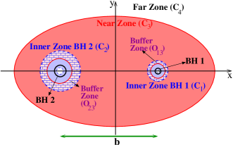
Figure 1: Schematic diagram of the near zone (dark gray), inner zones (light gray) and buffer zones (checkered) projected onto the orbital plane. The black holes’ horizons are shown by solid black lines, while the excision boundaries are shown by dashed black lines. The near zone overlaps the inner zone of each black hole, and these overlap regions are the buffer zones (checkered patterns.) The boundaries of all zones are somewhat imprecise since they are based on power series approximations, but the buffer zones are roughly spherical shells shown in this Figure as annuli.

The manifold is subdivided in such a way so that approximate solutions to the Einstein equations can be found in each region. These approximate solutions will depend on certain coordinates and parameters local only to that region. The near zone metric, $g_{\mu\nu}^{(3)}$, is an expansion in $\epsilon_{(3)}\equiv m/r\ll 1$, which depends on harmonic coordinates $x^{\mu}$ and parameters, such as the masses $m_{A}$ of the holes and the angular velocity $\omega$ of the system. Similarly, the metric in inner zone $1$ (or $2$), $h_{\bar{\mu}\bar{\nu}}^{(1)}$ (or $h_{\bar{\mu}\bar{\nu}}^{(2)}$), is an expansion in $\epsilon_{(1)}\equiv r_{1}/b\ll 1$ (or $\epsilon_{(2)}\equiv r_{2}/b\ll 1$), which depends on isotropic coordinates $x^{\bar{\mu}}$ and certain parameters, such as the mass of the background hole $M$ and the angular velocity $\Omega$ of the tidal perturbation. The parameters and the coordinates used in different regions are not identical and are valid only inside their respective regions, although those regions overlap.

A global metric can be obtained by relating the different approximate solutions through asymptotic matching. The theory of matched asymptotic expansions was first developed to perform multiple scale analysis on non-linear partial differential equations and to obtain global approximate solutions Bender and Orszag (1999). In general relativity, this method was first applied by Burke and Thorne Burke and Thorne (1970), Burke Burke (1971), and D’Eath D’Eath (1975a, b) in the $1970$s to derive corrections to the laws of motion due to coupling of the body’s motion to the geometry of the surrounding spacetime. Based on these ideas, in this paper we will develop a version of the theory of matched asymptotics that is useful to obtain initial data for numerical relativity simulations.

Asymptotic matching consists of relating different approximate solutions inside a common region of validity. This region is usually called the buffer zone by relativists, but is called the overlap region by others. For a binary there exists three such regions, which are $4$-volumes: Two buffer zones (${\cal{O}}_{13}$ and ${\cal{O}}_{23}$) are defined by the intersection of the near zone and the inner zones of black hole $1$ and $2$; the third one is defined by the intersection of the near zone and the radiation zone (${\cal{O}}_{34}$). The former two, shown in Fig. 1 in a checkered pattern, are defined by the asymptotic condition $m_{A}\ll r_{A}\ll b$. The latter has been analyzed in Ref. Blanchet (2006) and will not be discussed here. In this paper we perform asymptotic matching in the former two buffer zones $\mathcal{O}_{13}$ and $\mathcal{O}_{23}$. In order for our tidal perturbations in the inner zones to be valid, the inner zones $\mathcal{C}_{1}$ and $\mathcal{C}_{2}$ cannot overlap.

Once a buffer zone has been found, asymptotic matching can be used to relate adjacent approximate solutions. The first step is to find the asymptotic expansions of the approximate solutions inside the buffer zones. These approximate solutions depend on the expansion parameters, $\epsilon_{(1)}$, $\epsilon_{(2)}$ and $\epsilon_{(3)}$, which are small only in their respective regions of validity $\mathcal{C}_{1}$, $\mathcal{C}_{2}$, and $\mathcal{C}_{3}$. By definition, in each overlap region both expansion parameters are small, specifically ${\epsilon_{(1)}}\ll 1$ and $\epsilon_{(3)}\ll 1$ in ${\cal{O}}_{13}$, while ${\epsilon_{(2)}}\ll 1$ and $\epsilon_{(3)}\ll 1$ in ${\cal{O}}_{23}$. Inside buffer zone $1$, for example, we can then asymptotically expand the near zone solution in $\epsilon_{(1)}\ll 1$ to obtain $\tilde{g}_{\mu\nu}^{(3)}$ and the inner zone solution in ${\epsilon_{(3)}}\ll 1$ to obtain $\tilde{h}_{\bar{\mu}\bar{\nu}}^{(1)}$. These asymptotic expansions of approximate solutions are naturally bivariate since they depend on two independent expansion parameters. When working with these bivariate expansions, we use the symbol $O(p,q)$ both to denote terms of order $(m/b)^{p}(r_{A}/b)^{q}$ and uncontrolled remainders of order $(m/b)^{p}$ or $(r_{A}/b)^{q}$. Relating adjacent approximations then reduces to imposing the asymptotic matching condition

$$\tilde{g}_{\mu\nu}^{(3)}\sim\tilde{h}_{\bar{\mu}\bar{\nu}}\frac{\partial x^{\bar{\mu}}}{\partial x^{\mu}}\frac{\partial x^{\bar{\nu}}}{\partial x^{\nu}}.$$ (1)

This expression means not that the two approximate solutions are equated, which is correctly called “patching,” but rather that all coefficients of all controlled terms in the bivariate expansions are equated.

After imposing the asymptotic matching condition, one obtains a coordinate and parameter transformation between the near zone and the inner zone $1$ in ${\cal{O}}_{13}$ (and similarly in ${\cal{O}}_{23}$.) These transformations allow for the construction of a global piecewise metric, which is guaranteed to be asymptotically smooth in the buffer zone up to uncontrolled remainders in the matching scheme. Asymptotic smoothness here means that adjacent pieces of the piecewise global metric and all of their derivatives are asymptotic to each other inside the buffer zones. This asymptotic smoothness, however, does not rule out small discontinuities on the order of the uncontrolled remainders in the approximations, when we pass from one approximation to the other. The global metric can be made formally $C^{\infty}$ by smoothing over these discontinuities, which introduces a new error into the solution. Asymptotic smoothness, however, guarantees that this error will be smaller than or equal to that already contained in the uncontrolled remainders of the approximations, provided the smoothing functions are sufficiently well-behaved.

Finally, we enumerate the orders of approximation used in the near zone. The Einstein equations are guaranteed to generate a well-posed initial value problem for globally hyperbolic spacetimes Baumgarte and Shapiro (2003), where the initial data could consist of the extrinsic curvature $K_{ij}$ and the spatial $3$-metric $\gamma_{ij}=g_{ij}$. We can write the extrinsic curvature in the form

$$K_{ij}=\frac{1}{2\alpha}\left(2D_{(i}\beta_{j)}-\partial_{t}\gamma_{ij}\right),$$ (2)

where $\beta_{i}=g_{0i}$ is the shift vector and $\alpha$ is the lapse. Time derivatives are smaller than spatial derivatives by a characteristic velocity, which by the virial theorem is $O(m/b)^{1/2}$. Therefore to compute $K_{ij}$ consistently to a given order in $m/b$, the 4-metric components $g_{0i}$ are needed to $O(m/b)^{1/2}$ beyond the highest order in $g_{ij}$ (and $g_{00}$, which appears in $\alpha$). In this paper we compute the first two nonzero contributions to the $3$-metric and extrinsic curvature, i.e. the leading order terms and the lowest-order corrections. This means that we need the 4-metric components $g_{00}$ and $g_{ij}$ to $O(m/b)$, but we need $g_{0i}$ to $O(m/b)^{3/2}$. Note that this does not correspond to any standard post-Newtonian order counting or nomenclature, which is why we quote precisions and remainders precisely in terms of expansion parameters rather than in ambiguous terms such as “$n$th PN”. The standard post-Newtonian order counting corresponds to the calculation of the equations of motion for spinless bodies, but the counting must be altered when studying other problems, such as the bending of light or the equations of motion for bodies with spin Tagoshi et al. (2001).

III Near Zone Metric

In this section, we present the post-Newtonian (PN) metric in the near zone ${\cal C}_{3}$ and expand it in the overlap region $\mathcal{O}_{13}$, the buffer zone where the inner zone ${\cal C}_{1}$ of BH1 and the near zone overlap. When performing the matching in Sec. V, we will obtain the corresponding expansion in the other overlap region $\mathcal{O}_{23}$ by a simple symmetry transformation.

We use harmonic corotating coordinates $(t,x,y,z)$ rotating around the center of mass such that

$$t^{\prime} = t,$$

$$x^{\prime} = x\cos{\omega t}-y\sin{\omega t},$$

$$y^{\prime} = x\sin{\omega t}+y\cos{\omega t},$$

$$z^{\prime} = z,$$ (3)

where primed coordinates are nonrotating. The near-zone metric takes the form Blanchet et al. (1998)

$$g_{00}^{(3)} \approx -1+\frac{2m_{1}}{r_{1}}+\frac{2m_{2}}{r_{2}}+\omega^{2}(x^{2}+y^{2}),$$

$$g_{01}^{(3)} \approx -y\;\omega\left(1+\frac{2m_{1}}{r_{1}}\right),$$

$$g_{02}^{(3)} \approx x\;\omega\left(1+\frac{2m_{1}}{r_{1}}\right)-4\mu b\omega\left(\frac{1}{r_{1}}-\frac{1}{r_{2}}\right),$$

$$g_{ij}^{(3)} \approx \delta_{ij}\left(1+\frac{2m_{1}}{r_{1}}+\frac{2m_{2}}{r_{2}}\right),$$ (4)

where all remainders are at least $O(m/r)^{2}$ and the superscript reminds us we are working on submanifold ${\cal{C}}_{3}$. Here

$$r_{1}=\sqrt{x_{1}^{2}+y^{2}+z^{2}}=\sqrt{(x-m_{2}b/m)^{2}+y^{2}+z^{2}},$$

$$r_{2}=\sqrt{x_{2}^{2}+y^{2}+z^{2}}=\sqrt{(x+m_{1}b/m)^{2}+y^{2}+z^{2}}$$ (5)

are the usual harmonic radial coordinates centered on black holes 1 and 2 and $b$ is the separation between holes. Implicit in this metric is the assumption that $r_{A}$ (for $A=1,2$) is of order $b$, or in other words that the field point is not too close to one of the holes. (Recall that, in harmonic coordinates, the horizons are at $r_{A}=m_{A}$ if we neglect tidal deformations.) We do not include the $O(m/r)^{2}$ terms in $g_{00}$ in what is commonly called the first post-Newtonian (1PN) metric and we do include $O(m/r)^{3/2}$ terms in $g_{0i}$ for reasons discussed at the end of Sec. II. In Eq. (4) it is sufficient to use the first post-Newtonian approximation

$$\omega=\sqrt{\frac{m}{b^{3}}}\left[1-\frac{1}{2}\left(3-\frac{\mu}{m}\right)\frac{m}{b}+O\left(\frac{m}{b}\right)^{2}\right],$$ (6)

to the angular velocity, where $\mu=m_{1}m_{2}/(m_{1}+m_{2})$ is the reduced mass of the binary. Our choice of sign corresponds to coordinates in which the orbital angular momentum is in the positive $z$ direction, as shown in Fig. 2.

Figure 2: Diagram of the near zone coordinate system used for the post-Newtonian metric in harmonic coordinates. The $z$ axis is chosen parallel to the orbital angular momentum of the binary, so that the black holes orbit counter-clockwise here with angular velocity $\omega$. The origin is chosen to be the center of mass, while $r_{1}$ and $r_{2}$ denote the coordinate separations of the field point from hole 1 and 2 respectively. The coordinate separation between the holes is $b$.

We now concentrate on the overlap region (buffer zone) ${\cal O}_{13}$. Inside ${\cal O}_{13}$ we expand $1/r_{2}$ as a power series in $r_{1}$ as

$$\frac{1}{r_{2}}=\frac{1}{b}\sum_{n=0}^{\infty}(-1)^{n}\left(\frac{r_{1}}{b}\right)^{n}P_{n}\left(\frac{x_{1}}{r_{1}}\right),$$ (7)

where the $P_{n}$ are Legendre polynomials. Substituting into Eq. (4), we obtain

$$\tilde{g}_{00}^{(3)} \sim -1+\frac{2m_{1}}{r_{1}}+\frac{2m_{2}}{b}\left[1-\frac{r_{1}}{b}P_{1}\left(\frac{x_{1}}{r_{1}}\right)+\left(\frac{r_{1}}{b}\right)^{2}P_{2}\left(\frac{x_{1}}{r_{1}}\right)\right]+\omega^{2}\left(x^{2}+y^{2}\right),$$

$$\tilde{g}_{01}^{(3)} \sim -y\;\omega\left\{1+\frac{2m_{1}}{r_{1}}+\frac{2m_{2}}{b}\left[1-\frac{r_{1}}{b}P_{1}\left(\frac{x_{1}}{r_{1}}\right)\right]\right\},$$

$$\tilde{g}_{02}^{(3)} \sim x\;\omega\left\{1+\frac{2m_{1}}{r_{1}}+\frac{2m_{2}}{b}\left[1-{r_{1}\over{b}}P_{1}\left(\frac{x_{1}}{r_{1}}\right)\right]\right\}-4\mu b\omega\left\{{1\over{r_{1}}}-{1\over{b}}\left[1-{r_{1}\over{b}}P_{1}\left(\frac{x_{1}}{r_{1}}\right)+\left(r_{1}\over{b}\right)^{2}P_{2}\left(\frac{x_{1}}{r_{1}}\right)\right]\right\},$$

$$\tilde{g}_{03}^{(3)} \sim O(2,3),$$

$$\tilde{g}_{ij}^{(3)} \sim \delta_{ij}\left\{1+{2m_{1}\over{r_{1}}}+{2m_{2}\over{b}}\left[1-{r_{1}\over{b}}P_{1}\left(\frac{x_{1}}{r_{1}}\right)+\left(r_{1}\over{b}\right)^{2}P_{2}\left(\frac{x_{1}}{r_{1}}\right)\right]\right\},$$ (8)

where all errors are of order $O(2,3)$ and where $m_{1}\ll r_{1}\ll b$. The metric (8), denoted with a tilde, is the asymptotic expansion in the inner zone of BH1 of the PN metric, which is already an asymptotic expansion in the near zone.

Observe that these expansions constitute a series within a series (bivariate series). In order to see this more clearly, we can rearrange the spatial metric to get

$$\tilde{g}_{ij}^{(3)} \sim \delta_{ij}\left(1+{2m_{1}\over{r_{1}}}\left\{1+{m_{2}\over{m_{1}}}{r_{1}\over{b}}\left[1-{r_{1}\over{b}}\right.\right.\right.$$

$$\left.\left.\left.P_{1}\left(\frac{x_{1}}{r_{1}}\right)+\left({r_{1}\over{b}}\right)^{2}P_{2}\left(\frac{x_{1}}{r_{1}}\right)\right]\right\}\right),$$

$$\qquad m_{1}\ll r_{1}\ll b.$$

Equation (III) is a generalized Frobenius series Visser and Yunes (2003), where the expansion is about the regular singular points $r_{1}=0$ and $r_{1}=\infty$. There are clearly two independent perturbation parameters, namely $\epsilon_{(3)}=m_{1}/r_{1}$ (the usual PN expansion parameter used in ${\cal{C}}_{3}$) and $\epsilon_{(1)}=r_{1}/b$ (a tidal perturbation parameter used in ${\cal{C}_{1}}$). In the overlap region ${\cal{O}}_{13}$ we can expand in both.

IV Inner Zone Metric

In this section we discuss the metric in the inner zone ${\cal{C}}_{1}$ of BH1 and its asymptotic expansion in the overlap region ${\cal{O}}_{13}$.

Physically, we expect the spacetime in the inner zone of BH1 to be Schwarzschild with mass $M_{1}$ plus a tidal perturbation due to BH2. Thorne and Hartle Thorne and Hartle (1985) argue that, in the local asymptotic rest frame (LARF) of BH1, the metric can be expanded in powers of $M_{1}$ outside the horizon of BH1. The first term, independent of $M_{1}$, can be taken to represent the external universe and thus can be computed by placing a test particle in the spacetime of BH2 as done by Alvi Alvi (2000). This is the tidal perturbation due to BH2. Terms of higher order in $M_{1}$ describe BH1 itself (the Schwarzschild metric) and interactions between BH1 and BH2 (tidally-induced quadrupole, etc). At the level of approximation of this paper, we can neglect the interaction terms because they are $O(2,1)$ or higher.

Alvi identifies LARF coordinates, in terms of which the tidal perturbation is obtained, with isotropic coordinates (Fig. 3).

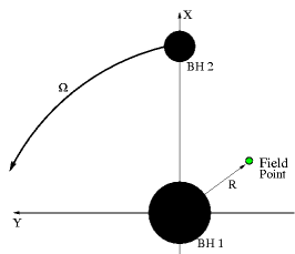
Figure 3: Coordinate system used in inner zone 1. The isotropic coordinates are centered on black hole $1$ and the other hole orbits with angular velocity $\Omega$. The matching parameters $M_{1}$ and $\Omega$ and the coordinates $X^{\mu}$ need not be equal to those used in the near zone.

Observe that this coordinate system is centered on BH1 and is inertial. The asymptotic form of the inner-zone tidally perturbed metric valid in the buffer zone is given by Eq. (3.14) of Alvi Alvi (2000), who derives it by extending Thorne-Hartle type arguments. But to serve as initial data the perturbation is needed throughout all the inner zone including the strong-field region, not just in the buffer zone where the field is weak. Alvi derives a form of the perturbation valid everywhere in the inner zone and presents it in Eq. (3.23) of Ref. Alvi (2000). The result depends on parameters $M_{1}$ and $\Omega$ which will be related to the near-zone parameters $m_{1}$ and $\omega$ when we perform the matching.

We write Eq. (3.23) of Ref. Alvi (2000) as

$$h_{00}^{IC,(1)} \approx -\left[{1-{M_{1}/(2R_{1})}}\over{1+{M_{1}/(2R_{1})}}\right]^{2}+{m_{2}\over{b^{3}}}\left(1-{M_{1}\over{2R_{1}}}\right)^{4}\left[3\left(X\cos{\Omega T}+Y\sin{\Omega T}\right)^{2}-R_{1}^{2}\right],$$

$$h_{01}^{IC,(1)} \approx {2m_{2}\over{b^{3}}}\sqrt{m\over{b}}\left(1-{M_{1}\over{2R_{1}}}\right)^{2}\left(1+{M_{1}\over{2R_{1}}}\right)^{4}\left[\left(Z^{2}-Y^{2}\right)\sin{\Omega T}-XY\cos{\Omega T}\right],$$

$$h_{02}^{IC,(1)} \approx {2m_{2}\over{b^{3}}}\sqrt{m\over{b}}\left(1-{M_{1}\over{2R_{1}}}\right)^{2}\left(1+{M_{1}\over{2R_{1}}}\right)^{4}\left[\left(X^{2}-Z^{2}\right)\cos{\Omega T}+XY\sin{\Omega T}\right],$$

$$h_{03}^{IC,(1)} \approx {2m_{2}\over{b^{3}}}\sqrt{m\over{b}}\left(1-{M_{1}\over{2R_{1}}}\right)^{2}\left(1+{M_{1}\over{2R_{1}}}\right)^{4}\left(Y\cos{\Omega T}-X\sin{\Omega T}\right)Z,$$

$$h_{ij}^{IC,(1)} \approx \left(1+{M_{1}\over{2R_{1}}}\right)^{4}\left(\delta_{ij}+{m_{2}\over{b^{3}}}\left[3\left(X\cos{\Omega T}+Y\sin{\Omega T}\right)^{2}-R_{1}^{2}\right]\left\{\left[\left(1+{M_{1}\over{2R_{1}}}\right)^{4}-{2M_{1}^{2}\over{R_{1}^{2}}}\right]\delta_{ij}\right.\right.$$ (10)

$$\left.\left.-{2M_{1}\over{R_{1}}}\left(1+{M_{1}^{2}\over{4R_{1}^{2}}}\right){X^{i}X^{j}\over{R_{1}^{2}}}\right\}\right),$$

where once more the superscript $(1)$ is to remind us that this metric is valid in submanifold ${\cal{C}}_{1}$, while the $IC$ superscript refers to isotropic coordinates. The uncontrolled remainders in all components of Eq. (10) are $O(R_{1}/b)^{3}$.

Inspection of Eq. (10) shows that the perturbed metric diverges as $R_{1}\to 0$ faster than $(1/R_{1})^{4}$, which prevents the use of puncture methods Tichy et al. (2003a). Physically, this is because the tidal perturbation tacitly assumes a small spacelike separation from the event horizon. Of course this assumption is violated as $R_{1}\to\infty$, the asymptotically flat spatial infinity we call the “outside” of hole 1; but it is also violated as $R_{1}\to 0$ since, in isotropic coordinates, that is the other asymptotically flat spatial infinity “inside” hole 1. Outside the hole we match to the near zone metric which is well behaved, but inside we have nothing to match to. Thus numerical evolutions using our initial data will need to excise the black holes. Excision in practice still requires a slice that extends somewhat inside each horizon, which raises the question of how far inside our data can be considered valid. Outside hole A the tidal perturbation is valid for $R_{A}\ll(m_{A}/m)b$. The corresponding limit inside the hole is approximated by the transformation $R_{A}\to(m_{A}/2)^{2}/R_{A}$, which is an isometry for an unperturbed Schwarzschild hole, where we have used $m_{A}\approx M_{A}$. Thus the tidal perturbation is good roughly for

$${m_{A}\over 2}{m\over 2b}\ll R_{A}\ll{m_{A}\over m}b,$$ (11)

and the excision radius can be chosen anywhere between the lower limit of this expression and the horizon.

Since matching will be simpler if performed between two coordinate systems that live in charts that are similar to each other, we choose to corotate first. We define inner isotropic corotating coordinates (ICC)

$$\bar{X} = X\cos{\Omega T}+Y\sin{\Omega T},$$

$$\bar{Y} = -X\sin{\Omega T}+Y\cos{\Omega T},$$

$$\bar{Z} = Z,$$

$$\bar{T} = T.$$ (12)

Using these equations, we can obtain the inner metric in isotropic corotating coordinates, given by

$$h^{(1)}_{00} \approx H_{t}+H_{s1}\Omega^{2}\left(\bar{X}^{2}+\bar{Y}^{2}\right)$$

$$+2H_{st}\bar{X}{\Omega\over{b^{2}}}\left(\bar{X}^{2}+\bar{Y}^{2}-\bar{Z}^{2}\right),$$

$$h^{(1)}_{11} \approx H_{s1}-H_{s2}{\bar{X}^{2}\over{b^{2}}},$$

$$h^{(1)}_{01} \approx -H_{s1}\bar{Y}\Omega-H_{st}{\bar{Y}\bar{X}\over{b^{2}}},$$

$$h^{(1)}_{22} \approx H_{s1}-H_{s2}{\bar{Y}^{2}\over{b^{2}}},$$

$$h^{(1)}_{02} \approx H_{s1}\bar{X}\Omega+{H_{st}\over{b^{2}}}\left(\bar{X}^{2}-\bar{Z}^{2}\right),$$

$$h^{(1)}_{33} \approx H_{s1}-H_{s2}{\bar{Z}^{2}\over{b^{2}}},$$

$$h^{(1)}_{03} \approx H_{st}{\bar{Y}\bar{Z}\over{b^{2}}},$$

$$h^{(1)}_{12} \approx -H_{s2}{\bar{Y}\bar{X}\over{b^{2}}},$$

$$h^{(1)}_{23} \approx -H_{s2}{\bar{Z}\bar{Y}\over{b^{2}}},$$

$$h^{(1)}_{13} \approx -H_{s2}{\bar{Z}\bar{X}\over{b^{2}}},$$ (13)

where we use the shorthand

$$H_{st} = 2m_{2}\sqrt{\frac{m}{b^{3}}}\left(1-{M_{1}\over{2R_{1}}}\right)^{2}\left(1+{M_{1}\over{2R_{1}}}\right)^{4},$$

$$H_{s1} = \left(1+{M_{1}\over{2R_{1}}}\right)^{4}\left\{1+2{m_{2}\over{b^{3}}}R_{1}^{2}P_{2}\left({\bar{X}\over{R_{1}}}\right)\right.$$

$$\left.\left[\left(1+{M_{1}\over{2R_{1}}}\right)^{4}-2{M_{1}^{2}\over{R_{1}^{2}}}\right]\right\},$$

$$H_{s2} = \left(1+{M_{1}\over{2R_{1}}}\right)^{4}\left(1+{M_{1}^{2}\over{4R_{1}^{2}}}\right){4m_{2}M_{1}\over{bR_{1}}}P_{2}\left({\bar{X}\over{R_{1}}}\right),$$

$$H_{t} = -\left({1-M_{1}/2R_{1}}\over{1+M_{1}/2R_{1}}\right)^{2}+2\left(1-{M_{1}\over{2R_{1}}}\right)^{4}$$ (14)

$${m_{2}\over{b^{3}}}R_{1}^{2}P_{2}\left({\bar{X}\over{R_{1}}}\right),$$

and the errors are still $O(R_{1}/b)^{3}$. In Eq. (IV) we have dropped the superscript ICC in favor of (1), which refers to submanifold ${\cal{C}}_{1}$.

By expanding Eq. (IV) in powers of $M_{1}/R_{1}$, which is permissible in overlap region $\mathcal{O}_{13}$, we obtain

$$\tilde{h}_{00}^{(1)} \sim -1+{2M_{1}\over{R_{1}}}+{2m_{2}\over{b^{3}}}R_{1}^{2}P_{2}\left(\bar{X}\over{R_{1}}\right)$$

$$+\Omega^{2}\left(\bar{X}^{2}+\bar{Y}^{2}\right),$$

$$\tilde{h}_{01}^{(1)} \sim {-2m_{2}\over{b^{3}}}\sqrt{\frac{m}{b}}\bar{Y}\bar{X}-\bar{Y}\Omega\left(1+{2M_{1}\over{R_{1}}}\right),$$

$$\tilde{h}_{02}^{(1)} \sim {2m_{2}\over{b^{3}}}\sqrt{\frac{m}{b}}\left(\bar{X}^{2}-\bar{Z}^{2}\right)+\bar{X}\Omega\left(1+{2M_{1}\over{R_{1}}}\right),$$

$$\tilde{h}_{03}^{(1)} \sim {2m_{2}\over{b^{3}}}\sqrt{\frac{m}{b}}\bar{Z}\bar{Y},$$

$$\tilde{h}_{ij}^{(1)} \sim \delta_{ij}\left[1+{2M_{1}\over{R_{1}}}+{2m_{2}\over{b^{3}}}R_{1}^{2}P_{2}\left(\bar{X}\over{R_{1}}\right)\right]$$ (15)

where the errors are $O(2,3)$. Like Eq. (8), ${\tilde{h}}_{\mu\nu}^{(1)}$ is a bivariate expansion in both $\epsilon_{(1)}=R_{1}/b$ (valid in the inner zone ${\cal{C}}_{1}$) and $\epsilon_{(3)}=M_{1}/R_{1}$ (valid in the buffer zone ${\cal{O}}_{13}$). In other words, it is the asymptotic expansion in the buffer zone to the asymptotic expansion in the inner zone.

V Asymptotic Matching

In this section, we concentrate on finding a matching condition ($\psi_{13}$) and a coordinate transformation ($\phi_{13}$) that maps points in ${\cal{C}}_{1}$ labeled with isotropic corotating coordinates (ICC) $\bar{X}^{\mu}$ to points in ${\cal{C}}_{3}$ labeled with harmonic corotating coordinates (HCC) $x^{\mu}$. As already discussed, we concentrate on buffer zone ${\cal{O}}_{13}$, while the matching condition $\psi_{23}$ and the coordinate transformation $\phi_{23}$ in ${\cal{O}}_{23}$ will be given later by a symmetry transformation.

We assume that the coordinates are asymptotic to each other and that they can be expanded in an implicit bivariate series. That is, we assume that the map $\phi_{13}:{\bar{X}}^{\mu}\to x^{\mu}$ has the form

$$\bar{X} \approx \left(x-{m_{2}b\over{m}}\right)+x\left[\left(m_{2}\over{b}\right)^{1/2}\chi_{1}(x^{\mu})+\left(m_{2}\over{b}\right)\chi_{2}(x^{\mu})+\left(m_{2}\over{b}\right)^{3/2}\chi_{3}(x^{\mu})\right],$$

$$\bar{Y} \approx y\left[1+\left(m_{2}\over{b}\right)^{1/2}\gamma_{1}(x^{\mu})+\left(m_{2}\over{b}\right)\gamma_{2}(x^{\mu})+\left(m_{2}\over{b}\right)^{3/2}\gamma_{3}(x^{\mu})\right],$$

$$\bar{Z} \approx z\left[1+\left(m_{2}\over{b}\right)^{1/2}\zeta_{1}(x^{\mu})+\left(m_{2}\over{b}\right)\zeta_{2}(x^{\mu})+\left(m_{2}\over{b}\right)^{3/2}\zeta_{3}(x^{\mu})\right],$$

$$\bar{T} \approx t\left[1+\left(m_{2}\over{b}\right)^{1/2}\tau_{1}(x^{\mu})+\left(m_{2}\over{b}\right)\tau_{2}(x^{\mu})+\left(m_{2}\over{b}\right)^{3/2}\tau_{3}(x^{\mu})\right],$$ (16)

where $\chi$, $\gamma$, $\zeta$ and $\tau$ are functions of the harmonic corotating coordinates which do not depend on $m/b$ (or equivalently $\omega$), but are power series in $r_{1}/b$. We continue these power series only to $O(r_{1}/b)^{2}$ so that the errors here in $\phi_{13}$ are $O(2,3)$ as in Eqs. (8) and (IV) which are linked by $\phi_{13}$. The first term in the $\bar{X}$ equation above is chosen so that both coordinate systems have their origins at the center of mass of the binary.

Like the coordinates, the matching parameters in the two coordinate systems must be identical to lowest order in $m_{2}/b$. (They must also be independent of coordinates.) Then $\psi_{13}$ is given by

$$M_{1} \approx m_{1}\left[1+\left(m_{2}\over{b}\right)^{1/2}\eta_{1}+{m_{2}\over{b}}\eta_{2}+\left(m_{2}\over{b}\right)^{3/2}\eta_{3}\right],$$

$$\Omega \approx \omega\left[1+\left(m_{2}\over{b}\right)^{1/2}\kappa_{1}+{m_{2}\over{b}}\kappa_{2}+\left(m_{2}\over{b}\right)^{3/2}\kappa_{3}\right],$$

where the errors are $O(m/b)^{2}$.

Before moving on with the calculation, let us discuss the physical meaning of the assumptions we have just made. Equation (16) implies that inner and near zone metrics are identical in the buffer zone up to a change in coordinates. For a single black hole, in the buffer zone (which is outside the horizon), the only difference between isotropic and harmonic coordinates is the radial transformation

$$r=R\left(1+{M^{2}\over 4R^{2}}\right),$$ (18)

where $r$ is in harmonic coordinates and $R$ is in isotropic coordinates. This has the asymptotic form posited in Eq. (16). Thus the assumption of Eq. (16) is only needed in the buffer zone for the matching in this section. However, we will want to write our final results in a global coordinate system which goes inside the horizons (though not all the way to the asymptotically flat ends). For this purpose we assume that the form of Eq. (16) holds for all values of $r_{1}>0$. This has the effect of defining a new coordinate system which is asymptotic to harmonic coordinates in the near zone and to isotropic coordinates in the inner zone.

Now let us return to the asymptotic matching. Using Eq. (V) we can transform Eq. (IV) to harmonic corotating coordinates and impose the matching condition of Eq. (1),

$$\tilde{g}_{\mu\nu}^{(3)}(x^{\gamma})\sim\tilde{h}_{\alpha\beta}^{(1)}\left(\bar{X}^{\gamma}\left(x^{\gamma}\right)\right){{\partial\bar{X}^{\alpha}}\over{\partial x^{\mu}}}{{\partial\bar{X}^{\beta}}\over{\partial x^{\nu}}}.$$ (19)

Equation (19) provides $10$ independent asymptotic relations per order, all of which must be satisfied simultaneously. Each asymptotic relation results in a first-order partial differential equation for the coordinate transformation, leading to $10$ integration constants per order. As we shall see, these constants correspond to boosts, rotations, and translations of the origin.

Equation (19) must be solved iteratively in orders of $(m/b)^{1/2}$. Evaluating the nonzero components (the diagonals) of Eq. (19) at zeroth order in $m/b$, i.e. comparing Eqs. (8) and (IV), provides no information, since it only asserts that at lowest order both metrics represent Minkowski spacetime. This is true for any matching formulation involving metrics of objects that would have asymptotically flat spacetimes in isolation.

The asymptotic relations given by evaluating Eqs. (8), (IV), and (19) at $O(m/b)^{1/2}$ are

$$\chi_{1}\sim-x\chi_{1,x}, \zeta_{1}\sim-z\zeta_{1,z}$$

$$\gamma_{1}\sim-y\gamma_{1,y}, \tau_{1}\sim-t\tau_{1,t},$$

$$t\tau_{1,x}\sim x\chi_{1,t}, y\gamma_{1,t}-t\tau_{1,y}\sim\left(m_{2}\over{m}\right)^{1/2},$$

$$t\tau_{1,z}\sim z\zeta_{1,t}, x\chi_{1,y}\sim-y\gamma_{1,x},$$

$$z\zeta_{1,x}\sim-x\chi_{1,z}, y\gamma_{1,z}\sim-z\zeta_{1,y},$$ (20)

where commas stand for partial differentiation. The solution in terms of integration constants $C_{i}$ is

$$t\tau_{1}(x,y,z,t) = C_{4}x+C_{5}y-\sqrt{m_{2}/m}\,y+C_{8}z+C_{9},$$

$$x\chi_{1}(x,y,z,t) = -C_{1}y+C_{2}z+C_{4}t+C_{3},$$

$$y\gamma_{1}(x,y,z,t) = -C_{1}x+C_{7}z+C_{5}t+C_{6},$$

$$z\zeta_{1}(x,y,z,t) = -C_{2}x-C_{7}y+C_{8}t+C_{10}.$$ (21)

For simplicity, we choose all $C_{i}=0$ except $C_{5}=\sqrt{m_{2}/m}$. Thus the coordinate systems are identical at $O(m/b)^{1/2}$. The coordinate transformation then becomes

$$\bar{X} \approx \left(x-{m_{2}b\over{m}}\right)+x\left[\left(m_{2}\over{b}\right)\chi_{2}(x^{\mu})\right.$$

$$\left.+\left(m_{2}\over{b}\right)^{3/2}\chi_{3}(x^{\mu})\right],$$

$$\bar{Y} \approx y\left[1+\left(m_{2}\over{b}\right)\gamma_{2}(x^{\mu})+\left(m_{2}\over{b}\right)^{3/2}\gamma_{3}(x^{\mu})\right],$$

$$+\sqrt{\frac{m_{2}}{b}}\sqrt{\frac{m_{2}}{m}}t,$$

$$\bar{Z} \approx z\left[1+\left(m_{2}\over{b}\right)\zeta_{2}(x^{\mu})+\left(m_{2}\over{b}\right)^{3/2}\zeta_{3}(x^{\mu})\right],$$

$$\bar{T} \approx t\left[1+\left(m_{2}\over{b}\right)\tau_{2}(x^{\mu})+\left(m_{2}\over{b}\right)^{3/2}\tau_{3}(x^{\mu})\right],$$ (22)

where the errors are still $O(2,3)$.

Applying asymptotic matching to $O(m/b)$, we obtain

$$-\left(\tau_{2}+t\tau_{2,t}\right) \sim 1-\frac{(x-m_{2}b/m)}{b}=1-\frac{x_{1}}{b},$$

$$\chi_{2}+x\chi_{2,x} \sim 1-\frac{(x-m_{2}b/m)}{b}=1-\frac{x_{1}}{b},$$

$$\gamma_{2}+y\gamma_{2,y} \sim 1-\frac{(x-m_{2}b/m)}{b}=1-\frac{x_{1}}{b},$$

$$\zeta_{2}+z\zeta_{2,z} \sim 1-\frac{(x-m_{2}b/m)}{b}=1-\frac{x_{1}}{b},$$

$$x\chi_{2,t}-t\tau_{2,x} \sim {t\over{b}}+\left(m\over{m_{2}}\right)^{1/2}{y\over{b}}\kappa_{1},$$

$$y\gamma_{2,t}-t\tau_{2,y} \sim -\left(m\over{m_{2}}\right)^{1/2}{x-m_{2}b/m\over{b}}\kappa_{1},$$

$$z\zeta_{2,t} \sim t\tau_{2,z},$$

$$x\chi_{2,y} \sim -y\gamma_{2,x},$$

$$x\chi_{2,z} \sim -z\zeta_{2,x},$$

$$\gamma_{2,z} \sim -z\zeta_{2,y}.$$ (23)

Once more we have a system of $10$ coupled partial differential equations that now depends on $\kappa_{1}$, which is a parameter that relates $\Omega$ and $\omega$. For simplicity, we choose $\kappa_{1}=0$, so that the $\Omega=\omega$ to this order. The solution to this system is then given by

$$\tau_{2} = -\left[1-{x\over{b}}+\frac{m_{2}}{m}\right]+D_{5}{y\over{t}}+D_{4}{x\over{t}}+D_{8}{z\over{t}}+{D_{9}\over{t}},$$

$$\chi_{2} = 1-{x\over{2b}}+\frac{m_{2}}{m}+{1\over{2xb}}\left(2t^{2}+y^{2}+z^{2}\right)+D_{1}{y\over{x}}+D_{4}{t\over{x}}+D_{2}{z\over{x}}+{D_{3}\over{x}},$$

$$\gamma_{2} = 1-{x\over{b}}+\frac{m_{2}}{m}-D_{1}{x\over{y}}+D_{7}{z\over{y}}+D_{5}{t\over{y}}+{D_{6}\over{y}},$$

$$\zeta_{2} = 1-{x\over{b}}+\frac{m_{2}}{m}+D_{8}{t\over{z}}-D_{7}{y\over{z}}-D_{2}{x\over{z}}+{D_{10}\over{z}},$$ (24)

where the $D_{i}$ are 10 more integration constants. For simplicity we set them to zero, and the coordinate transformation becomes

$$\bar{X} \approx \left(x-{m_{2}b\over{m}}\right)+x\left\{\left(m_{2}\over{b}\right)\left[1-{(x-2m_{2}b/m)\over{2b}}\right]+\left(m_{2}\over{b}\right)^{3/2}\chi_{3}(x^{\mu})\right\}+{m_{2}\over{2b^{2}}}\left(2t^{2}+y^{2}+z^{2}\right),$$

$$\bar{Y} \approx y\left\{1+\left(m_{2}\over{b}\right)\left[1-{(x-m_{2}b)/m\over{b}}\right]+\left(m_{2}\over{b}\right)^{3/2}\gamma_{3}(x^{\mu})\right\}+\sqrt{\frac{m_{2}}{b}}\sqrt{\frac{m_{2}}{m}}t,$$

$$\bar{Z} \approx z\left\{1+\left(m_{2}\over{b}\right)\left[1-{(x-m_{2}b)/m\over{b}}\right]+\left(m_{2}\over{b}\right)^{3/2}\zeta_{3}(x^{\mu})\right\},$$

$$\bar{T} \approx t\left\{1-\left(m_{2}\over{b}\right)\left[1-{(x-m_{2}b/m)\over{b}}\right]+\left(m_{2}\over{b}\right)^{3/2}\tau_{3}(x^{\mu})\right\},$$ (25)

with errors of $O(2,3)$.

Now that matching has been completed to $O(m/b)^{0}$, $O(m/b)^{1/2}$ and $O(m/b)$, we can proceed with matching at $O(m/b)^{3/2}$. However, keeping in mind our discussion in Sec. II of the orders needed, we will only use the spatial-temporal part of the asymptotic relations matrix (19),

$$x\chi_{3,t}-t\tau_{3,x} \sim -\left(m\over{m_{2}}\right)^{1/2}\left[{y\over{b}}\left(1-\kappa_{2}-{4x\over{b}}+3{m_{2}\over{m}}\right)\right],$$

$$t\tau_{3,y}-y\gamma_{3,t} \sim \left(m\over{m_{2}}\right)^{1/2}\Biggl{(}{x\over{b}}\left[\kappa_{2}-1+\frac{4m_{1}-6m_{2}}{m}-4\left(\frac{m_{2}}{m}\right)^{2}+8\frac{\mu}{m}\right]+\left(\frac{x}{b}\right)^{2}\left(\frac{7}{2}-\frac{4m_{1}}{m}+\frac{2m_{2}}{m}\right)\Biggr{.}$$

$$\Biggl{.}+\left(\frac{y}{b}\right)^{2}\left(-\frac{1}{2}-\frac{m_{2}}{m}+\frac{2m_{1}}{m}\right)+\left(\frac{z}{b}\right)^{2}\left(-\frac{3}{2}-\frac{m_{2}}{m}+\frac{2m_{1}}{m}\right)+\left(\frac{t}{b}\right)^{2}+\frac{4\mu b}{m_{2}r_{1}}\Biggr{.}$$

$$\Biggl{.}+\left\{\frac{m_{2}}{m}\left[1-\kappa_{2}+2\left(\frac{m_{2}}{m}\right)^{2}+\frac{3m_{2}-4\mu}{m}\right]-\frac{9\mu+8m_{1}}{2m}+\frac{3}{2}\right\}\Biggr{)},$$

$$t\tau_{3,z}-z\zeta_{3,t} \sim \left(m\over{m_{2}}\right)^{1/2}{zy\over{b^{2}}}.$$ (26)

For simplicity, we choose $\kappa_{2}=1+3m_{2}/m$. This completes the derivation of the matching parameters, since $\eta_{i}$ and $\kappa_{3}$ did not appear in the differential equations at all, and hence, we can neglect them to this order. Note that this choice of parameter matching is different from Alvi’s choice, and thus our coordinate transformation is also different. Up to $O(m/b)^{2}$, the corresponding parameter matching condition $\psi_{13}$ is

$$\Omega\approx\omega\left[1+{m_{2}\over{b}}\left(1+3{m_{2}\over{m}}\right)\right],\quad M_{1}\approx m_{1}.$$ (27)

This choice of $\psi_{13}$ simplifies Eq. (26), which now becomes

$$t\tau_{3,x}-x\chi_{3,t} \sim -\left(m\over{m_{2}}\right)^{1/2}{4yx\over{b^{2}}},$$

$$t\tau_{3,z}-z\zeta_{3,t} \sim \left(m\over{m_{2}}\right)^{1/2}{zy\over{b^{2}}},$$

$$t\tau_{3,y}-y\gamma_{3,t} \sim \left(m\over{m_{2}}\right)^{1/2}\Biggl{(}{x\over{b}}\left[\frac{4m_{1}-3m_{2}}{m}-4\left(\frac{m_{2}}{m}\right)^{2}+8\frac{\mu}{m}\right]+\left(\frac{x}{b}\right)^{2}\left(\frac{7}{2}-\frac{4m_{1}}{m}+\frac{2m_{2}}{m}\right)\Biggr{.}$$ (28)

$$\Biggl{.}+\left(\frac{y}{b}\right)^{2}\left(-\frac{1}{2}-\frac{m_{2}}{m}+\frac{2m_{1}}{m}\right)+\left(\frac{z}{b}\right)^{2}\left(-\frac{3}{2}-\frac{m_{2}}{m}+\frac{2m_{1}}{m}\right)+\left(\frac{t}{b}\right)^{2}+\frac{4\mu b}{m_{2}r_{1}}\Biggr{.}$$

$$\Biggl{.}+\left\{\frac{m_{2}}{m}\left[2\left(\frac{m_{2}}{m}\right)^{2}-\frac{4\mu}{m}\right]-\frac{9\mu+8m_{1}}{2m}+\frac{3}{2}\right\}\Biggr{)}.$$

As before, we choose the integration constants for simplicity (and to keep the slicings close to each other), resulting in the following solution:

$$\tau_{3}(x,y,z,t) = 0,$$

$$\chi_{3}(x,y,z,t) = \left(m\over{m_{2}}\right)^{1/2}{4yt\over{b^{2}}},$$

$$\zeta_{3}(x,y,z,t) = -\left(m\over{m_{2}}\right)^{1/2}{yt\over{b^{2}}},$$

$$\gamma_{3}(x,y,z,t) = -\left(m\over{m_{2}}\right)^{1/2}{t\over{y}}\Biggl{(}{x\over{b}}\left[\frac{4m_{1}-3m_{2}}{m}-4\left(\frac{m_{2}}{m}\right)^{2}+8\frac{\mu}{m}\right]+\left(\frac{x}{b}\right)^{2}\left(\frac{7}{2}-\frac{4m_{1}}{m}+\frac{2m_{2}}{m}\right)\Biggr{.}$$ (29)

$$\Biggl{.}+\left(\frac{y}{b}\right)^{2}\left(-\frac{1}{2}-\frac{m_{2}}{m}+\frac{2m_{1}}{m}\right)+\left(\frac{z}{b}\right)^{2}\left(-\frac{3}{2}-\frac{m_{2}}{m}+\frac{2m_{1}}{m}\right)+\frac{1}{3}\left(\frac{t}{b}\right)^{2}+\frac{4\mu b}{m_{2}r_{1}}\Biggr{.}$$

$$\Biggl{.}+\left\{\frac{m_{2}}{m}\left[2\left(\frac{m_{2}}{m}\right)^{2}-\frac{4\mu}{m}\right]-\frac{9\mu+8m_{1}}{2m}+\frac{3}{2}\right\}\Biggr{)}.$$

To summarize, we have found a coordinate transformation $\phi_{13}$ and a set of parameter relations $\psi_{13}$ that produce asymptotic matching to $O(3/2,3)$ in the $00$ and $ij$ components of the 4-metric and to $O(2,3)$ in the $0i$ components.

Note however that the $\gamma_{3}$ piece of the coordinate transformation becomes singular at $r_{1}=0$. Also recall that the point $r_{1}=0$ is not identical to the point $R_{1}=0$, where the inner zone metric perturbation diverges. Hence if we excise the inner zone metric close to $R_{1}=0$, the point $r_{1}=0$ might be outside the excised region, in which case our coordinate transformation would introduce a coordinate singularity outside the excised region. To get rid of this singularity we will replace $r_{1}$ by

$$\tilde{r}_{1}=\sqrt{r_{1}^{2}+6m^{2}}.$$ (30)

This change amounts to adding a higher order term to the coordinate transformation, which has no effect in the buffer zone at the current order of approximation, but it has the advantage that the resulting coordinate transformation is now regular at $r_{1}=0$. With this replacement the coordinate transformation is given by

$$\bar{X} \approx \left(x-{m_{2}b\over{m}}\right)+x\left\{\left(m_{2}\over{b}\right)\left[1-{(x-2m_{2}b/m)\over{2b}}\right]+\frac{m_{2}}{b}\sqrt{\frac{m}{b}}{4yt\over{b^{2}}}\right\}+{m_{2}\over{2b^{2}}}\left(2t^{2}+y^{2}+z^{2}\right),$$

$$\bar{Y} \approx y\left\{1+\left(m_{2}\over{b}\right)\left[1-{x-m_{2}b/m\over{b}}\right]\right\}-\frac{m_{2}}{b}\sqrt{\frac{m}{b}}t\Biggl{(}{x\over{b}}\left[\frac{4m_{1}-3m_{2}}{m}-4\left(\frac{m_{2}}{m}\right)^{2}+8\frac{\mu}{m}\right]+\left(\frac{x}{b}\right)^{2}\left(\frac{7}{2}-\frac{4m_{1}}{m}+\frac{2m_{2}}{m}\right)\Biggr{.}$$

$$\Biggl{.}+\left(\frac{y}{b}\right)^{2}\left(-\frac{1}{2}-\frac{m_{2}}{m}+\frac{2m_{1}}{m}\right)+\left(\frac{z}{b}\right)^{2}\left(-\frac{3}{2}-\frac{m_{2}}{m}+\frac{2m_{1}}{m}\right)+\frac{1}{3}\left(\frac{t}{b}\right)^{2}+\frac{4\mu b}{m_{2}\tilde{r}_{1}}+\left\{\frac{m_{2}}{m}\left[2\left(\frac{m_{2}}{m}\right)^{2}-\frac{4\mu}{m}\right]\right.\Biggr{.}$$

$$\left.\Biggl{.}-\frac{9\mu+8m_{1}}{2m}+\frac{3}{2}\right\}\Biggr{)}+\sqrt{\frac{m_{2}}{m}}\sqrt{\frac{m_{2}}{b}}t,$$

$$\bar{Z} \approx z\left\{1+\left(m_{2}\over{b}\right)\left[1-{x-m_{2}b/m\over{b}}\right]-\frac{m_{2}}{b}\sqrt{\frac{m}{b}}{yt\over{b^{2}}}\right\},$$

$$\bar{T} \approx t\left\{1-\left(m_{2}\over{b}\right)\left[1-{x-m_{2}b/m\over{b}}\right]\right\},$$

$$\Omega \approx \omega\left[1+{m_{2}\over{b}}\left(1+3{m_{2}\over{m}}\right)\right],$$

$$M_{1} \approx m_{1}.$$ (31)

The coordinate transformation for matching in the other overlap region $\mathcal{O}_{23}$ is obtained by the following symmetry transformation:

$$1\leftrightarrow 2,\qquad x\to-x,\qquad y\to-y,\qquad z\to z.$$ (32)

In Eq. (V), $t$ should be considered small just as $x$, $y$, and $z$ are. Recall that fundamentally the overlap regions are 4-volumes, although when we choose a time slicing we have to deal with their projections on a spatial hypersurface ($m_{A}\ll r_{A}\ll b$). Just as the overlap regions span a limited range of $r_{A}$, so they span a limited range of $t$. The post-Newtonian metric and the perturbed Schwarzschild metric are formally stationary, but the true physical system includes gravitational waves (not modeled here) which for example change the orbital frequency on a radiation reaction timescale. While this timescale is longer than an orbital period, which must be of order $b$, rotation and boosts mix space and time terms and to be consistent with $r_{A}\ll b$ we must keep $t\ll b$. Therefore we choose the $t=0=T$ slice when discussing the approximate metric in the next section, which restricts our overlap region to the intersection of this 3-surface with the overlap 4-volume.

VI An approximate metric for binary black holes

In this section we transform the inner zone metric in isotropic corotating coordinates to harmonic corotating coordinates via Eq. (V). The metric in the inner zone of black hole $1$ is given by

$$g_{\mu\nu}^{(1)}=h_{\bar{\delta}\bar{\rho}}^{(1)}J^{\bar{\delta}}{}_{\mu}J^{\bar{\rho}}{}_{\nu},$$ (33)

where in the buffer zone the $g_{00}$ and $g_{ij}$ components have errors of $O(2,3)$ and $g_{0i}$ has errors of $O(5/2,3)$. In the above equation the Jacobian $J^{\bar{\mu}}{}_{\nu}=\partial_{\nu}\bar{X}^{\bar{\mu}}$ can be expanded as

$$J^{\bar{T}}{}_{t} = 1-{m_{2}\over{b}}\left(1-{x-m_{2}b/m\over{b}}\right),$$

$$J^{\bar{T}}{}_{x} = {m_{2}t\over{b^{2}}},$$

$$J^{\bar{X}}{}_{t} = {m_{2}\over{b}}\left({2t\over{b}}+4{xy\omega\over{b}}\right),$$

$$J^{\bar{X}}{}_{x} = 1+{m_{2}\over{b}}\left(1-{x-m_{2}b/m\over{b}}+{4\omega yt\over{b}}\right),$$

$$J^{\bar{X}}{}_{y} = {m_{2}\over{b}}\left({y\over{b}}+4{x\omega t\over{b}}\right),$$

$$J^{\bar{X}}{}_{z} = {m_{2}z\over{b^{2}}},$$

$$J^{\bar{Y}}{}_{t} = \sqrt{m_{2}\over{m}}\sqrt{m_{2}\over{b}}-\frac{m_{2}}{b}\sqrt{m\over{b}}\left\{\frac{x}{b}\left[\frac{4m_{1}-3m_{2}}{m}-4\left(\frac{m_{2}}{m}\right)^{2}+8\frac{\mu}{m}\right]+\left(\frac{x}{b}\right)^{2}\left(\frac{7}{2}-\frac{4m_{1}}{m}+\frac{2m_{2}}{m}\right)+\left(\frac{y}{b}\right)^{2}\left(-\frac{1}{2}\right.\right.$$

$$\left.\left.-\frac{m_{2}}{m}+\frac{2m_{1}}{m}\right)\left(\frac{z}{b}\right)^{2}\left(-\frac{3}{2}-\frac{m_{2}}{m}+\frac{2m_{1}}{m}\right)+\left(\frac{t}{b}\right)^{2}+\frac{4\mu b}{m_{2}{\tilde{r}}_{1}}+\frac{m_{2}}{m}\left[2\left(\frac{m_{2}}{m}\right)^{2}-4\frac{\mu}{m}\right]-\frac{9\mu+8m_{1}}{2m}-\frac{3}{2}\right\},$$

$$J^{\bar{Y}}{}_{x} = {-m_{2}\over{b}}{y\over{b}}-\frac{m_{2}}{b}\sqrt{m\over{b}}\frac{t}{b}\left\{\left[\frac{4m_{1}-3m_{2}}{m}-4\left(\frac{m_{2}}{m}\right)^{2}+8\frac{\mu}{m}\right]+\frac{2x}{b}\left(\frac{7}{2}-\frac{4m_{1}}{m}+\frac{2m_{2}}{m}\right)-4\frac{\mu b^{2}}{m_{2}}\frac{x-m_{2}b/m}{{\tilde{r}}_{1}^{3}}\right\},$$

$$J^{\bar{Y}}{}_{y} = 1+{m_{2}\over{b}}\left(1-{x-m_{2}b/m\over{b}}\right)-\frac{m_{2}}{b}\sqrt{m\over{b}}t\left[\frac{2y}{b^{2}}\left(-\frac{1}{2}-\frac{m_{2}}{m}+\frac{2m_{1}}{m}\right)-4\frac{\mu b}{m_{2}}\frac{y}{{\tilde{r}}_{1}^{3}}\right],$$

$$J^{\bar{Y}}{}_{z} = -\frac{m_{2}}{b}\sqrt{m\over{b}}t\left[\frac{2z}{b^{2}}\left(-\frac{3}{2}-\frac{m_{2}}{m}+2\frac{m_{1}}{m}\right)-4\frac{\mu b}{m_{2}}\frac{z}{{\tilde{r}}_{1}^{3}}\right],$$

$$J^{\bar{Z}}{}_{t} = -\frac{m_{2}}{b}\sqrt{m\over{b}}{zy\over{b^{2}}},$$

$$J^{\bar{Z}}{}_{x} = -m_{2}{z\over{b^{2}}},$$

$$J^{\bar{Z}}{}_{y} = -\frac{m_{2}}{b}\sqrt{m\over{b}}{zt\over{b^{2}}},$$

$$J^{\bar{Z}}{}_{z} = 1+{m_{2}\over{b}}\left(1-{x-m_{2}b/m\over{b}}\right)-\frac{m_{2}}{b}\sqrt{m\over{b}}{yt\over{b^{2}}}.$$ (34)

Furthermore, $h_{\mu\nu}^{(1)}$ refers to the inner metric presented in Eq. (IV), where we substitute the coordinate transformation given by Eq. (V) and

$$R_{1}=\left(\bar{X}^{2}+\bar{Y}^{2}+\bar{Z}^{2}\right)^{1/2}.$$ (35)

The metric in the inner zone of black hole $2$ (${\cal{C}}_{2}$) is given by the symmetry transformation (32) applied to Eq. (33).

We now have all the ingredients to construct an approximate piecewise metric, for example

$$g_{\mu\nu}^{piece} \approx \left\{\begin{array}[]{ll}g_{\mu\nu}^{(1)},\qquad r_{1}<r_{1}^{T}\\ g_{\mu\nu}^{(2)},\qquad r_{2}<r_{2}^{T}\\ g_{\mu\nu}^{(3)},\qquad r_{1}>r_{1}^{T},r_{2}>r_{2}^{T},r<\lambda/2\pi\end{array}\right.$$ (39)

for some transition radii $r_{A}^{T}$ which are chosen to be inside ${\cal O}_{A3}$ for $A=\{1,2\}$. In Eq. (39), $g_{\mu\nu}^{(3)}$ is given in Eq. (4), $g_{\mu\nu}^{(1)}$ is given in Eq. (33) and $g_{\mu\nu}^{(2)}$ is the symmetry transformed version of Eq. (33). The inner zone pieces of this metric are accurate to $O(R_{1}/b)^{2}$, while the post-Newtonian near zone pieces are accurate to $O(m/r)^{3/2}$. In the overlap region, the inner and near zone $0i$ components asymptotically match up to $O(3/2,2)$ as required for the extrinsic curvature, while all other components asymptotically match only up to $O(1,2)$.

Note that when we applied the coordinate transformation of Eq. (V) to the inner zone metric we kept terms up to $O(m/b)^{5}$, which at first glance seems too high. These terms are needed because the inner zone metric represents a tidally perturbed black hole with errors in the physics of $O[(m/b)(R_{1}/b)^{3}]$. Close to BH1 ($R_{1}\sim m$), the error in the physics is only of order $O(m/b)^{4}$ and hence we should keep terms to at least order $O(m/b)^{3}$. However, recall that the perturbed black hole metric satisfies the Einstein equations up to errors of only $O[(m/b)^{5/2}(R_{1}/b)^{2}]$ even though its astrophysical resemblance to a binary black hole has errors already at $O[(m/b)(R_{1}/b)^{3}]$. If we want to obtain a metric which is close to the constraint hypersurface, we should keep terms larger than $O[(m/b)(R_{1}/b)^{3}]$, but not larger than $O[(m/b)^{5/2}(R_{1}/b)^{2}]$. In particular, close to the black hole we have constraint violations of $O(m/b)^{9/2}$. For example, if we had dropped terms of order $O(m/b)^{4}$ in the inner zone metric we would have introduced additional constraint violations at this order.

VI.1 Global character of the asymptotic metric

In this subsection we plot Eq. (39) to describe some features of the approximate piecewise metric. We choose a system of equal-mass black holes $m_{1}=m_{2}=m/2$ separated by $b=10m$, so that both holes are located on the $x$ axis with BH1 at $x\approx 5m$ and BH2 at $x\approx-5m$. Figures 4 and 5 show the $xx$ and $00$ components of the metric along the $x$ axis for this system. (Other components of the piecewise $4$-metric exhibit similar behavior.) In all plots we use a dashed line to denote the near zone metric ($g_{\mu\nu}^{(3)}$) and dotted lines to denote the inner zone metrics ($g_{\mu\nu}^{(1,2)}$) We choose the separation $b=10m$ because it is near the minimum for which our formalism makes sense, and we plot on the $x$-axis because it is where the worst behavior occurs. The idea is to (i) show some practical features of matching which have not been presented in the literature and (ii) demonstrate the limits of the method, particularly regarding the minimum separation.

In these plots, we also include error bars that estimate the uncontrolled remainders in the approximations. These remainders can be approximated by

$$2[(m_{1}/r_{1})^{2}+(m_{2}/r_{2})^{2}]$$ (40)

in the near zone,

$$2(m_{2}/b)(R_{1}/b)^{3}$$ (41)

in inner zone 1, and the same with $1\leftrightarrow 2$ for inner zone 2. The error in the near zone metric was estimated by looking at the next order (2PN) term in the metric components Blanchet et al. (1998). [That term is much more complicated than Eq. (40), but is numerically about equal to it in the region plotted.] The error in the inner zone metric comes about because the next tidal correction for a single black hole of mass $m$ in perturbation theory will be roughly proportional to ${1\over{3}}R_{i0j0,k}$. The error bars of the approximations are position-dependent, and thus provide a useful sign of where each approximation is breaking down. The PN error bars are larger near the holes than far away, and the BHPT error bars exhibit the opposite behavior. The error bars also provide an indicator of where both approximations are comparably good: Neglecting angular factors (as is typical in the literature), the error bars for the near zone and inner zone $A$ are comparable at

$$r^{T}_{A}\approx\left(b^{4}m_{A}^{2}/m\right)^{1/5},$$ (42)

which takes a value of about $4.8m$ for the system plotted here. This radius is a good candidate for the “transition radius” of Eq. (39), but note that, in principle, there is an infinite number of possible candidates, as long as they are in the buffer zone. Furthermore, note that this is not a “matching radius,” since there is no such thing. Matching asymptotic expansions, as opposed to patching them as done by Alvi Alvi (2000), does not happen at any particular place in the buffer zone. Rather, it makes two expansions comparable throughout the buffer zone up to the uncontrolled remainders.

In Figs. 4 and 5 we plot the $xx$ and $00$ metric components along the $x$-axis for the PN approximation as well as for the two perturbed black hole approximations. In Fig. 1 the buffer zones around each black hole were sketched as spherical shells around the holes, formally defined by $m_{1}\ll r_{1}\ll b$ and $m_{2}\ll r_{2}\ll b$. It is important to recall that this definition, which is ubiquitous in the literature, is imprecise because of the $\ll$ symbols and one cannot simply substitute $<$ symbols. (For one thing, there is angular dependence of the uncontrolled remainders.) Inserting the parameters of our system into these definitions, in Fig. 4 the intersection of buffer zone 1 with the $x$-axis is given by $5.5\ll x/m\ll 15$ (to the right of BH1) and $-5\ll x/m\ll 4.5$ (to the left, between the holes). In the part of the buffer zone to the right, away from BH2, we see a clean example of the behavior expected of matched asymptotic expansions: The near-zone curve and the BH1 inner-zone curve do not intersect, but the difference between them is comparable to the estimated error bars everywhere within this part of the buffer zone, even if we replace the $\ll$ operator in the definition of the buffer zone by the precise $<$ operator.

Between the holes, to the left in Fig. 4, the interpretation of the curves is not so simple. We cannot replace $\ll$ by $<$ in the definition of buffer zone 1 because to the left of $x/m\approx 0$ ($r_{1}\approx b/2$) the near-zone metric component resembles that of BH2 rather than BH1. This is because $m_{1}\ll r_{1}\ll b$ is a rough criterion obtained by ignoring (among other things) the angular dependence of the expansion coefficients in Eq. (8), inspection of which shows about a factor of two variation as the angle is changed. This angular dependence means that if one tries to redefine the buffer zone heuristically as “the region where the error bars on two curves overlap and are not too large,” it is significantly aspherical and can be squeezed out entirely. Even at the origin (where they are smallest), the error bars from the PN approximation in the near zone are visibly larger than they are for most of the right-hand part of buffer zone 1. These error bars, however, are what is expected: At the origin in Fig. 4 the $O(m/r)$ term which is kept in the PN metric has a value of 0.4, for a total metric component of $g_{xx}^{(3)}=1.4$. The uncontrolled $O(m/r)^{2}$ term we use for the error bar is 0.04, which is precisely 10% of the $m/b$ correction and about twice the value at $x/m=\pm 10$, a comparable distance on the other side of each hole. The fact that the error bars are worst in between the holes does not depend on $m/b$ or the mass ratio, but rather is a reflection of the physical assumptions on which matching is based. The near-zone metric is matched in buffer zone 1 to the metric of inner zone 1, and in buffer zone 2 it is matched to the metric of inner zone 2, but inner zone 1 is never matched to inner zone 2. It is the intervening near zone that ensures that each black hole’s tidal perturbation is the appropriate one (up to uncontrolled remainders) for the other black hole, because each tidal perturbation is derived for a black hole without a nearby body. (See, for example, the discussion in Sec. II.B of Thorne and Hartle Thorne and Hartle (1985).)

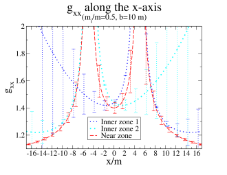
Figure 4: This figure shows the $xx$ component of the near zone metric (PN), denoted by a dashed line, and the inner zone metrics (BHPT), denoted by dotted lines, along the (harmonic) $x$ axis for a perturbative parameter $m/b=1/10$, with the black holes located at $x/m=\pm 5$. The buffer zones cannot be precisely defined, but most of the region plotted is within one or the other (see text). Matching does not guarantee that two curves which are asymptotically matched intersect anywhere in the buffer zone, but rather that they are comparable at the level of the uncontrolled remainders. The error bars estimate these remainders as described in the text.

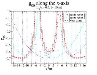
Figure 5: This figure is similar to Fig. 4, but it shows the $00$ component of the metric. Observe that in this component the differences between the different approximations are more pronounced, although the general features of asymptotic matching are still discernible.

Since the inner-zone and near-zone metric components diverge as $r_{A}\to 0$, Fig. 4 might seem to imply that the solutions approach each other near the horizons. This misconception can be rectified by scaling the solutions to the Brill-Lindquist factor $\psi^{4}$, where

$$\psi=1+{m_{1}\over{2r_{1}}}+{m_{2}\over{2r_{2}}}.$$ (43)

This removes most of the divergent behavior of the solutions, as shown in Fig. 6. In this figure, we only plot the region near BH $1$ to show the difference in divergence better, but the region near BH $2$ is very similar.

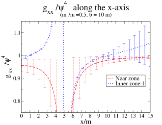
Figure 6: In this figure we plot the $xx$ component of the near zone (PN - dashed line) and inner zone $1$ (BHPT -dotted line) metrics divided by the Brill-Lindquist factor $\psi^{4}$. The behavior of the solutions is clearly different as we approach the event horizon from the left (the direction of the other hole).

To the right, away from the other black hole, we see that the near-zone and inner-zone solutions are indeed quite similar near BH1 and that there is a wide region where both sets of error bars are comparable and overlap. The transition radius $r^{T}_{1}\approx 4.8m$ ($x/m\approx 10$) discussed above is seen to be a good approximation of where the error bars are equal. To the left, between the holes, there is only a small region (about $|x|/m<1$) where the error bars overlap, and they are never equal.

The smallness of the region where the error bars overlap is an indication that $b=10m$ is approaching the minimum separation for which our approximation method makes sense. The disappearance of such a region could be used as a criterion for the failure of matching, although this is not a standard test and several different approximate criteria could be used (and this region is not the formal definition of a buffer zone anyway.) In Fig. 5 the error bars never do quite overlap at $x/m\approx 0$, but they do overlap at $x/m\approx\pm 1$, although we must keep in mind that they are rough estimates. As discussed above, the error bars cannot be made equal at the origin by changing $m/b$, although the overlap can be made better by increasing the separation. The fact that the rescaled metric components in Fig. 6 take off in different directions as they approach BH1 from between the holes is partly because the two metrics blow up at different coordinate locations. This small relative translation is due to the coordinate system used in the matching.

VI.2 Transition Functions

The fact that matched curves do not strictly overlap even in the buffer zone means that a piecewise metric such as Eq. (39) possesses discontinuities at the transition radii $r^{T}_{A}$, wherever they are chosen to be. These discontinuities can be problematic for numerical evolutions of the spacetime and thus it is desirable to smooth them. We now construct transition functions that smooth these discontinuities out, by letting

$$g_{\mu\nu}^{(1,3)}=\left[1-F_{1}(R_{1})\right]g_{\mu\nu}^{(1)}+F_{1}(R_{1})g_{\mu\nu}^{(3)},$$ (44)

where $F_{1}$ has the properties that $F_{1}(R_{1}\gtrsim b)=1$, $F_{1}(R_{1}\lesssim m_{1})=0$, $F_{1}(R_{1}\approx r_{1}^{T})\approx 1/2$. This ansatz yields a metric that is equal to the inner zone metric near black hole 1, while it is equal to the near zone metric far away from black hole 1. In between (i.e. in the buffer zone) we obtain a weighted average of these two solutions. Since the Einstein equations are nonlinear, the sum of two solutions is in general not another solution. But since both solutions are valid in the buffer zone, and since both have been matched, these two solutions are equal to each other in the buffer zone up to uncontrolled remainders of $O(2,3)$, corresponding to higher order post-Newtonian and tidal perturbation terms. Hence any weighted average of these two solutions in the buffer zone will yield the same correct solution up to uncontrolled remainders of $O(2,3)$. This justifies the use of smoothing to merge the two solutions in the buffer zone. A similar solution can be obtained for the other black hole by replacing $1\to 2$.

We choose transition functions of the form

$$f(r)=\left\{\begin{array}[]{ll}0,\qquad r\leq r_{0}\\ \frac{1}{2}\left\{1+\tanh\left[\frac{s}{\pi}\left(\tan(\frac{\pi}{2w}(r-r_{0}))\right.\right.\right.\\ \left.\left.\left.-\frac{q^{2}}{\tan(\frac{\pi}{2w}(r-r_{0}))}\right)\right]\right\},\qquad r_{0}<r<r_{0}+w\\ 1,\ \qquad r\geq r_{0}+w.\end{array}\right.$$ (49)

This function transitions from zero to one in a transition window which starts at $r_{0}$ and has a width $w$. The parameter $q$ controls the location at which $f$ reaches 1/2, and $s$ controls the slope at that location. Note that this transition function is $C^{\infty}$, a property which is useful for numerics. In Eq. (44) we set

$$F_{A}(R_{A})=f(R_{A}),$$ (50)

with parameters

$$r_{0}=1.5m,\qquad w=5r^{T}_{A},\qquad q=1/4,\qquad s=10,$$ (51)

where $r^{T}_{A}$ is given by Eq. (42). With these parameters the transition functions reach the value $1/2$ at $R_{A}\approx 1.5m+0.16w\approx 5.2m$, very close to $r^{T}_{A}\approx 4.8m$. We could have used something more sophisticated such as a transition with the same anisotropic behavior as the buffer zones, but several trials show that such details do not matter as long as the transition function has the right asymptotic properties. (Trials also showed that the results were not too sensitive to the precise parameter values.)

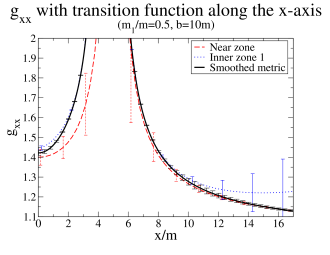
Figure 7: In this figure we show the $xx$ component of the global metric compared to the near-zone PN metric and the inner-zone BHPT metric around BH1. Observe that the transition function takes the global metric smoothly from one to the other. Error bars in the global metric are the same as the error bars of whichever local approximation is better at that point.

We can see the effect of this transition function in Fig. 7 and 8. In these figures we only show the region near BH $1$, but similar behavior is observed near the other hole. The transition function effectively takes one solution into the other smoothly in the buffer zone. The size of the transition window can be modified by changing the “thickness” $w$, but if $w$ is made too small the derivatives of the metric (which include $1/w$ terms) develop artificial peaks inside the transition window.

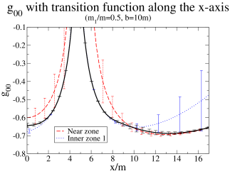
Figure 8: Same as the previous Figure, but for the $00$ metric component.

If the separation of the black holes is large enough so that the two transition windows of width $w$ do not intersect, the transition functions given in Eq. (49) will suffice to generate a global metric of the form

$$g_{\mu\nu}^{(global)} = F_{2}(R_{2})F_{1}(R_{1})g_{\mu\nu}^{(3)}+\left[1-F_{1}(R_{1})\right]g_{\mu\nu}^{(1)}$$ (52)

$$+\left[1-F_{2}(R_{2})\right]g_{\mu\nu}^{(2)},$$

However, if the separation is small enough that the two transition windows of width $w$ start to overlap, we must construct a third function $G(x)$ to allow for a smooth transition between the two black holes while not contaminating the global solution near BH1 with a piece of the solution from inner zone 2 and vice versa. (In essence, this is an after the fact way of handling the fact that the buffer zones are not really spherically symmetric as often implied in the literature. When the holes are too close, a good transition function should not be spherically symmetric either.) For the system considered here, $b=10m$ is a sufficiently small separation that such a third transition function is necessary. The global metric then becomes

$$g_{\mu\nu}^{(global)} = G(x)\left\{F_{1}(R_{1})g_{\mu\nu}^{(3)}+\left[1-F_{1}(R_{1})\right]g_{\mu\nu}^{(1)}\right\}$$ (53)

$$+\left[1-G(x)\right]\left\{F_{2}(R_{2})g_{\mu\nu}^{(3)}+\left[1\right.\right.$$

$$\left.\left.-F_{2}(R_{2})\right]g_{\mu\nu}^{(2)}\right\}.$$

(Recall that $x$ is the distance along the axis between the holes with the origin at the center of mass.) The function $G(x)$ will be chosen such that it is equal to unity near black hole $1$ and zero near black hole $2$. In between the two black holes, $G(x)$ will range from zero to one, so that non-trivial averaging will occur only in this region. Again, this averaging is allowed because the two solutions in the curly brackets are both valid (and equal up to uncontrolled remainders) in between the two black holes. Near each black hole we obtain the appropriate inner zone solution, while far away $F_{1}(R_{1})=F_{2}(R_{2})=1$, so that we obtain the near zone solution $g_{\mu\nu}^{(3)}$. We choose the transition function $G(x)$ between ${\cal{C}}_{1}\cup{\cal{C}}_{3}$ and ${\cal{C}}_{2}\cup{\cal{C}}_{3}$ to be of the same form as the function in Eq. (49), i.e.

$$G(x)=f(x),$$ (54)

but with different parameter values

$$r_{0}=\frac{b(m_{2}-m_{1})}{2m}-\frac{b-m}{2},\;w=b-m,\;q=1,\;s=5/2.$$ (55)

(The more complicated form of $r_{0}$ is to account for the origin of the $x$ coordinate being at the binary center of mass rather than on either hole.)

The reader might worry that the use of transition functions could introduce large artificial gradients. However, with a reasonable choice of transition functions this is not the case. In order to understand why, let us look at the derivatives of the smoothed metric in more detail. Consider for example the overlap region $\mathcal{O}_{13}$ in which $F_{2}=1$ and the smoothed metric is thus $F_{1}g_{\mu\nu}^{(3)}+\left[1-F_{1}\right]g_{\mu\nu}^{(1)}$. A derivative of this smoothed metric takes the form

$$F_{1}g_{\mu\nu}^{(3)^{\prime}}+\left[1-F_{1}\right]g_{\mu\nu}^{(1)^{\prime}}+F_{1}^{\prime}\left[g_{\mu\nu}^{(3)}-g_{\mu\nu}^{(1)}\right].$$ (56)

The last term is the worrying one since it involves a derivative of the transition function. But note that the coefficient multiplying this term is the difference between the inner-zone and near-zone metrics in the buffer zone, and therefore is by definition of the order of the uncontrolled remainders in the expansions of the first two terms. Therefore the third (unphysical) term will be safely absorbed into the small uncontrolled remainders unless we make a pathological choice of transition function—for example, one that has an inverse power of a small expansion parameter built into it. Our transition functions are chosen to avoid this. Their maximum slope is roughly $1/r^{T}_{A}$, comparable to the slopes of $g_{\mu\nu}^{(1)}$ and $g_{\mu\nu}^{(3)}$ in the vicinity of $r^{T}_{A}$ where the maximum occurs. Thus the unphysical third term in Eq. (56) is always formally small. (We demonstrate that it is also small in practice in Sec. VII.) The errors introduced into the constraint equations are found by differentiating (56). Again, all terms involving derivatives of the transition functions are multiplied by the differences between expanded metrics in the buffer zone, which are of the same order as the uncontrolled remainders and therefore can be neglected.

In Figs. 9 and 10, we demonstrate the good behavior of the smoothed solution.

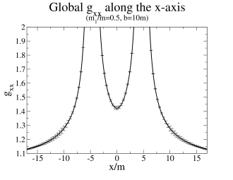
Figure 9: This figure shows the $xx$ component of the global approximation of the metric across both holes.

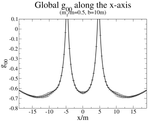
Figure 10: Same as the previous Figure, but for the $00$ metric component.

Observe that as $x$ increases, the global metric with the transition function becomes identical to the near zone metric, while as $r_{A}$ approaches zero (near each hole, $x/m\to\pm 5$) it becomes equal to the inner zone metric. Since the holes are close to each other, in the region between the holes the global metric never becomes identical to the near zone metric but rather always contains a contribution from the inner zone metrics. This linear combination is valid in that region because there the asymptotic expansions of both approximate metrics are comparable to each other. In Figs. 7 and 8, the error bars of the global metric with the transition function overlap the error bars of the inner and near zone metrics in the regions where the former are valid. This criterion would not be satisfied if the near zone and inner zone curves were farther from each other, which would occur if the holes were closer, and thus could be taken as another indicator that the holes are still (barely) far enough apart for matching.

VII Initial Data for Numerical Relativity

The approximate metric (53) could be used as initial data for binary black hole simulations. To facilitate this task we now present this metric in the $3+1$ decomposition, by providing explicit analytic expressions for the extrinsic curvature, lapse and shift on the ${\bar{T}}=t=0$ slice. If the normal vector to this slice is denoted by $n^{a}$, then the intrinsic metric in the slice is given by

$$q_{ab}=g_{ab}+n_{a}n_{b},$$ (57)

and the extrinsic curvature is

$$K_{ab}=-\frac{1}{2}\pounds_{n}q_{ab},$$ (58)

where $\pounds_{n}$ is the Lie derivative in the direction normal to the $t=0$-slice. Below we compute $K_{ab}$ using the explicit expression

$$K_{ab}=-\frac{1}{2}n^{c}\left(\partial_{c}q_{ab}-\partial_{a}q_{cb}-\partial_{b}q_{ac}\right),$$ (59)

which has been obtained using the ordinary derivative operator and the fact that $q_{ab}n^{b}=0$. The evolution vector

$$(\partial_{t})^{a}=\alpha n^{a}+\beta^{a}$$ (60)

is split into pieces perpendicular and parallel to the $t=0$ slice, where $\alpha$ denotes the lapse and $\beta^{a}$ the shift. Note that $n^{a}n_{a}=-1$ and $\beta^{a}n_{a}=0$.

The near zone extrinsic curvature computed from the PN metric Blanchet et al. (1998) in corotating harmonic coordinates on the $t=0$ slice is given by

$$K_{ij}^{(3)}=\sum_{A=1}^{2}m_{A}\frac{4v_{A}^{(i}n_{A}^{j)}-v_{A}^{k}n^{A}_{k}\delta_{ij}}{r_{A}^{2}},$$ (61)

where the error is of $O(m/b)^{5/2}$, the superscript $3$ is to remind us that this expression is only valid in ${\cal{C}}_{3}$, and where the parentheses on the indices stand for symmetrization. In the previous equation, $v_{A}^{i}$ and $n_{A}^{i}$ denotes the particle velocities and directional vectors given by

$$v_{1}^{2}=\omega\frac{m_{2}}{m}b,\qquad v_{2}^{2}=-\omega\frac{m_{1}}{m}b,\qquad v_{A}^{1}=v_{A}^{3}=0$$ (62)

and

$$n^{k}_{A}=\frac{x^{k}-x^{k}_{A}}{r_{A}},\ \ \ x^{1}_{1}=\frac{m_{2}}{m}b,\ \ x^{1}_{2}=-\frac{m_{1}}{m}b,\ \ x^{2}_{A}=x^{3}_{A}=0.$$ (63)

The corresponding near zone lapse and shift on the $t=0$ slice are

$$\alpha_{(3)}=1-\sum_{A=1}^{2}\frac{m_{A}}{r_{A}}$$ (64)

and

$$\beta_{(3)}^{i}=-\sum_{A=1}^{2}\frac{4m_{A}v_{A}^{i}}{r_{A}}-\epsilon_{ij3}\omega x^{j},$$ (65)

where once more this is valid on ${\cal{C}}_{3}$.

The extrinsic curvature of the $\bar{T}=0$ slice valid in the inner zone of black hole $1$ (${\cal{C}}_{1}$) and computed from the metric given in the previous section in isotropic corotating coordinates is

$$K_{00}^{(1),ICC} = -{m2\over{b^{3}}}\Omega^{2}\bar{Y}\left(\bar{X}^{2}+\bar{Y}^{2}\right){\Psi^{5}\over{\Psi-\frac{M_{1}}{R_{1}}}}\left[2\left(\Psi-\frac{M_{1}}{R_{1}}\right)^{2}b\omega+3\Omega\bar{X}\left(\Psi^{4}-{2M_{1}^{2}\over{R_{1}^{2}}}\right)\right],$$

$$K_{01}^{(1),ICC} = {m_{2}\over{b}}\Omega{\Psi^{5}\over{\Psi-\frac{M_{1}}{R_{1}}}}\left[3\Omega\bar{X}{\bar{Y}^{2}\over{b^{2}}}\left(\Psi^{4}-{2M_{1}^{2}\over{R_{1}^{2}}}\right)+\left(\Psi-\frac{M_{1}}{R_{1}}\right)^{2}{\omega\over{b}}(\bar{X}^{2}+2\bar{Y}^{2})+\left(\Psi-\frac{M_{1}}{R_{1}}\right)M_{1}\omega{\bar{X}^{2}\over{R^{3}b}}\right.$$

$$\left.\left(\bar{X}^{2}+\bar{Y}^{2}-\bar{Z}^{2}\right)\right],$$

$$K_{02}^{(1),ICC} = -{m_{2}\bar{X}\bar{Y}\over{b^{3}}}\Omega{\Psi^{5}\over{\Psi-\frac{M_{1}}{R_{1}}}}\left[\left(\Psi-\frac{M_{1}}{R_{1}}\right)^{2}b\omega+3\Omega\bar{X}\left(\Psi^{4}-{2M_{1}^{2}\over{R_{1}^{2}}}\right)-\left(\Psi-\frac{M_{1}}{R_{1}}\right){bM_{1}\over{R_{1}^{3}}}\omega\left(\bar{X}^{2}+\bar{Y}^{2}-\bar{Z}^{2}\right)\right],$$

$$K_{03}^{(1),ICC} = {m_{2}\over{b^{2}}}\omega\Omega\bar{X}\bar{Z}\Psi^{5}\left[{M_{1}\over{R_{1}^{3}}}\left(\bar{X}^{2}+\bar{Y}^{2}-\bar{Z}^{2}\right)-\Psi+\frac{M_{1}}{R_{1}}\right],$$

$$K_{11}^{(1),ICC} = -{m_{2}\bar{Y}\over{2b^{3}}}{\Psi^{5}\over{\Psi-\frac{M_{1}}{R_{1}}}}\left[4\left(\Psi-\frac{M_{1}}{R_{1}}\right)^{2}b\omega+4\left(\Psi-\frac{M_{1}}{R_{1}}\right)b{M_{1}\over{R_{1}^{3}}}\omega\bar{X}^{2}-3\Omega\bar{X}\left(4{M_{1}^{2}\over{R_{1}^{2}}}-2\Psi^{4}+{M_{1}^{3}\bar{X}^{2}\over{R_{1}^{5}}}\right.\right.$$

$$\left.\left.+{4M_{1}\bar{X}^{2}\over{R_{1}^{3}}}\right)\right],$$

$$K_{12}^{(1),ICC} = {m_{2}\bar{X}\over{2b^{3}}}{\Psi^{5}\over{\Psi-\frac{M_{1}}{R_{1}}}}\left[2\left(\Psi-\frac{M_{1}}{R_{1}}\right)^{2}b\omega+12M_{1}\Omega{\bar{X}\bar{Y}^{2}\over{R_{1}^{3}}}\left(1+{M_{1}^{2}\over{\left(\Psi-\frac{M_{1}}{R_{1}}\right)R_{1}^{2}}}\right)+2\left(\Psi-\frac{M_{1}}{R_{1}}\right)b\omega{M_{1}\over{R_{1}^{3}}}\right.$$ (66)

$$\left.\left(\bar{X}^{2}-\bar{Y}^{2}-\bar{Z}^{2}\right)\right],$$

$$K_{13}^{(1),ICC} = {6M_{1}m_{2}\Omega\bar{X}^{2}\bar{Y}\bar{Z}\over{b^{3}R_{1}^{3}}}{\Psi^{5}\over{\Psi-\frac{M_{1}}{R_{1}}}}\left(1+{M_{1}^{2}\over{4R_{1}^{2}}}\right),$$

$$K_{22}^{(1),ICC} = {m_{2}\bar{Y}\over{2b^{3}}}{\Psi^{5}\over{\Psi-\frac{M_{1}}{R_{1}}}}\left\{12{M_{1}^{2}\over{R_{1}^{2}}}\Omega\bar{X}-6\Omega\Psi^{4}\bar{X}+3{M_{1}^{3}\bar{Y}^{2}\over{R_{1}^{5}}}\Omega\bar{X}+4{M_{1}\over{R_{1}^{3}}}\left[3\Omega\bar{X}\bar{Y}^{2}+\left(\Psi-\frac{M_{1}}{R_{1}}\right)b\omega\left(\bar{X}^{2}-\bar{Z}^{2}\right)\right]\right\},$$

$$K_{23}^{(1),ICC} = -{m_{2}\bar{Z}\over{2b^{3}}}{\Psi^{5}\over{\Psi-\frac{M_{1}}{R_{1}}}}\left[2\left(\Psi-\frac{M_{1}}{R_{1}}\right)^{2}b\omega-12M_{1}\Omega{\bar{X}\bar{Y}^{2}\over{R_{1}^{3}}}\left(1+{M_{1}^{2}\over{4R_{1}^{2}}}\right)-2\left(\Psi-\frac{M_{1}}{R_{1}}\right){bM_{1}\omega\over{R_{1}^{3}}}\left(\bar{X}^{2}+\bar{Y}^{2}-\bar{Z}^{2}\right)\right],$$

$$K_{33}^{(1),ICC} = {m_{2}\bar{Y}\over{2b^{3}}}{\Psi^{5}\over{\Psi-\frac{M_{1}}{R_{1}}}}\left[4\left(\Psi-\frac{M_{1}}{R_{1}}\right)^{2}b\omega+4\left(\Psi-\frac{M_{1}}{R_{1}}\right)b\omega{M_{1}\bar{Z}^{2}\over{R_{1}^{3}}}+3\Omega\bar{X}\left(4{M_{1}^{2}\over{R_{1}^{2}}}-2\Psi^{4}+{M_{1}^{3}\bar{Z}^{2}\over{R_{1}^{5}}}+4{M_{1}\bar{Z}^{2}\over{R_{1}^{3}}}\right)\right],$$

where the error is of $O(R_{1}/b)^{3}$, and where the superscript $ICC$ is to remind that that this is calculated in isotropic corotating coordinates. Later on, we will transform this metric to harmonic corotating coordinates with the map $\phi_{13}$ found in Eq. (V), and we will drop this superscript. In the above equations, $\Psi$ is the Brill-Lindquist factor for black hole $1$ in isotropic coordinates, i.e.

$$\Psi=1+\frac{M_{1}}{2R_{1}}.$$ (67)

The $K_{0\mu}^{(1),ICC}$ components will be needed later in the coordinate transformation and are obtained from the purely spatial components $K_{kl}^{(1),ICC}$ using

$$K_{0\nu}^{(1),ICC}=q_{0}^{k}q_{\nu}^{l}K_{kl}^{(1),ICC},$$ (68)

where the projection tensor $q_{\mu}^{\nu}$ is given by

$$q_{\mu}^{\nu}=\delta_{\mu}^{\nu}+n^{(1),ICC}_{\mu}n_{(1),ICC}^{\nu}.$$ (69)

Here, the normal vector to the slice computed with $n^{(1),ICC}_{a}=-\sqrt{-1/h^{00}_{(1)}}(d\bar{T})_{a}$ is given by

$$n^{(1),ICC}_{0} = -\frac{{1-{M_{1}\over{2R_{1}}}}}{\Psi}\left[1-\frac{m_{2}}{b}\left(1-{M_{1}\over{2R_{1}}}\right)^{2}\Psi^{2}\frac{R_{1}^{2}}{b^{2}}P_{2}({\bar{X}\over{R_{1}}})\right],\qquad n^{(1),ICC}_{i}=0,$$ (70)

where $P_{2}$ stands for the second Legendre polynomial.

The upper components are then

$$n_{(1),ICC}^{0} = \frac{\Psi}{1-{M_{1}\over{2R_{1}}}}\left[1+\frac{m_{2}}{b}\left(1-{M_{1}\over{2R_{1}}}\right)^{2}\Psi^{2}\frac{R_{1}^{2}}{b^{2}}P_{2}(\bar{X}/R_{1})\right],$$

$$n_{(1),ICC}^{1} = \frac{\Psi}{1-{M_{1}\over{2R_{1}}}}\bar{Y}\left[\Omega+2\frac{m_{2}}{b}\omega\left(1-{M_{1}\over{2R_{1}}}\right)^{2}\frac{\bar{X}}{b}+\frac{m_{2}}{b}\Omega\left(1-{M_{1}\over{2R_{1}}}\right)^{2}\Psi^{2}\frac{R_{1}^{2}}{b^{2}}P_{2}(\bar{X}/R_{1})\right],$$

$$n_{(1),ICC}^{2} = -\frac{\Psi}{1-{M_{1}\over{2R_{1}}}}\left[\Omega\bar{X}+2\frac{m_{2}}{b}\omega\left(1-{M_{1}\over{2R_{1}}}\right)^{2}\frac{\bar{X}^{2}-\bar{Z}^{2}}{b}+\frac{m_{2}}{b}\Omega\left(1-{M_{1}\over{2R_{1}}}\right)^{2}\Psi^{2}\frac{R_{1}^{2}}{b^{2}}\bar{X}P_{2}(\bar{X}/R_{1})\right],$$

$$n_{(1),ICC}^{3} = -2\frac{m_{2}}{b}\omega\left(1-{M_{1}\over{2R_{1}}}\right)\Psi\frac{\bar{Y}\bar{Z}}{b}.$$ (71)

This means that the lapse and shift of the $\bar{T}=0$ slice in the inner zone (${\cal{C}}_{1}$) and in inner corotating coordinates are given by

$$\alpha_{(1),ICC} = -n^{(1),ICC}_{0}=\frac{1-{M_{1}\over{2R_{1}}}}{\Psi}\left[1-\frac{m_{2}}{b}\left(1-\right.\right.$$

$$\left.\left.{M_{1}\over{2R_{1}}}\right)^{2}\Psi^{2}\frac{R_{1}^{2}}{b^{2}}P_{2}(\bar{X}/R_{1})\right],$$

$$\beta_{(1),ICC}^{i} = -\alpha_{(1),ICC}n_{(1),ICC}^{i}.$$ (72)

Observe that the lapse of Eq. (72) goes through zero at $R_{1}=M/2$. Apart from a small perturbation it closely resembles the standard Schwarzschild lapse in isotropic coordinates.

Note that the extrinsic curvature, lapse and shift given up to this point are expressed in two different coordinate systems. The post-Newtonian quantities valid in the near zone (${\cal{C}}_{3}$) are given in harmonic corotating coordinates, while the black hole perturbation theory results valid in the inner zones (${\cal{C}}_{1,2}$) are given in isotropic corotating coordinates. We will now apply the coordinate transformation found in Sec. V, namely Eq. (V), to transform the inner zone expressions to harmonic corotating coordinates, thus dropping the label ICC in favor of the superscript $(1)$. The result for the inner extrinsic curvature of black hole $1$ is given by

$$K_{ij}^{(1)}=K_{\bar{l}\bar{m}}^{(1)}J^{\bar{l}}{}_{i}J^{\bar{m}}{}_{j},$$ (73)

where all components still have errors of $O(5/2,3)$. The extrinsic curvature in harmonic corotating coordinates in submanifold ${\cal{C}}_{2}$ can be obtained from the above equation by the symmetry transformation discussed in Eq. (32). In Fig. 11 we have plotted the $xy$ component of the extrinsic curvature along the $x$-axis. Observe that the behavior of the post-Newtonian solution (dashed line) is different from that of the black hole perturbation solution close to the black hole, where the latter diverges more abruptly. In Figs. 11–15, the error bars have been estimated by inserting Eqs. (40) and (41) into the definition of the quantity plotted and using $\partial_{t}r_{A}\approx b\omega$ and $\partial_{t}R_{A}\approx b\Omega$.

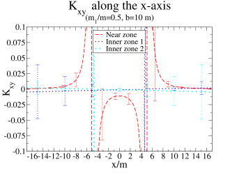
Figure 11: This figure shows the $xy$ component of the near zone (PN - dashed line) extrinsic curvature, as well as the inner zone curvatures (BHPT - dotted lines) obtained via black hole perturbation theory. This figure uses the same test case as previous figures, with equal mass black holes and $m/b=1/10$.

Similarly, the lapse and shift in harmonic corotating coordinates corresponding to the inner zone of black hole $1$ are given by

$$\alpha_{(1)} = \frac{1}{n_{(1)}^{0}}=-n^{(1)}_{0}=J^{\bar{T}}{}_{t}\alpha_{(1),ICC},$$

$$\beta^{i}_{(1)} = -\alpha_{1}n_{1}^{i},$$ (74)

where again the lapse and shift for the inner zone around black hole $2$ (${\cal{C}}_{2}$) can be obtained by the symmetry transformation (32). In these equations, the normal vector is given by

$$n_{(1)}^{\mu}=J^{\bar{\nu}}{}_{\nu}n_{(1),ICC}^{\nu},$$ (75)

where the matrix $J^{{\bar{\mu}}}{}_{\nu}$ has been defined in Eq. (VI). Note that $\alpha_{(1)}$ in Eq. (VII) has the same zeros as $\alpha_{(1),ICC}$ and, thus, $\alpha_{(1)}$ also changes sign at $R_{1}=M/2$. Furthermore, since $J^{\bar{T}}{}_{t}=1+O(m/b)$ the inner zone lapse $\alpha_{(1)}$ equals $\alpha_{(1),ICC}$ up to a perturbation of $O(m/b)$ and thus $\alpha_{(1)}$ is equal to the standard lapse of Schwarzschild in isotropic coordinates plus a perturbation of $O(m/b)$. These features are borne out by the plot in Fig. 12 which shows the global lapse along the x-axis. We can also see from the figure that while the inner zone lapse goes to $-1$ as $r_{1}\to 0$, the near zone one diverges to negative infinity.

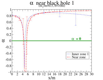
Figure 12: This figure shows the near zone (PN - dashed line) and the inner zone lapse (BHPT - dotted line) along the x-axis. Observe that the near zone lapse crosses zero at $x/m=5.5$ and $x/m=4.5$, which is the location of the event horizon in harmonic coordinates.

With these equations, we can construct an approximate piecewise global extrinsic curvature, lapse and shift by substituting the metric for these quantities in Eq. (39). By the theorems of asymptotic matching, the derivatives of adjacent pieces of the piecewise metric will be asymptotic to each other inside their respective buffer zones. This asymptotic similarity is, thus, also observed in the extrinsic curvature, as well as the lapse and the shift. Due to the piecewise nature of these solutions, there will be discontinuities on a $2$-sphere located at some transition radius inside of the buffer zone. In order to eliminate these discontinuities, we use the same transition functions used for the metric in Eq. (49) with the same parameters. In this manner, we obtain a smooth global extrinsic curvature, lapse and shift given by

$$K_{ij}^{(global)} = G(x)\left\{F_{1}(R_{1})K_{ij}^{(3)}+\left[1-F_{1}(R_{1})\right]K_{ij}^{(1)}\right\}+\left[1-G(x)\right]\left\{F_{2}(R_{2})K_{ij}^{(3)}+\left[1-F_{2}(R_{2})\right]K_{ij}^{(2)}\right\},$$

$$\alpha_{(global)} = G(x)\left\{F_{1}(R_{1})\alpha_{(3)}+\left[1-F_{1}(R_{1})\right]\alpha_{(1)}\right\}+\left[1-G(x)\right]\left\{F_{2}(R_{2})\alpha_{(3)}+\left[1-F_{2}(R_{2})\right]\alpha_{(2)}\right\},$$

$$\beta^{i}_{(global)} = G(x)\left\{F_{1}(R_{1})\beta^{i}_{(3)}+\left[1-F_{1}(R_{1})\right]\beta^{i}_{(1)}\right\}+\left[1-G(x)\right]\left\{F_{2}(R_{2})\beta^{i}_{(3)}+\left[1-F_{2}(R_{2})\right]\beta^{i}_{(2)}\right\}.$$ (76)

Figs. 13, 14 and 15 show the global lapse, shift and extrinsic curvature with the transition functions.

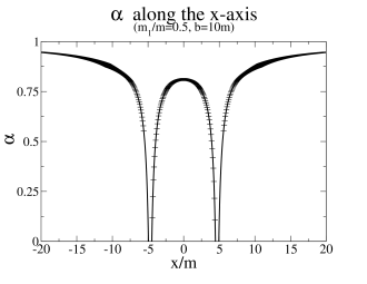
Figure 13: This figure shows the global lapse along the x-axis with the transition function.

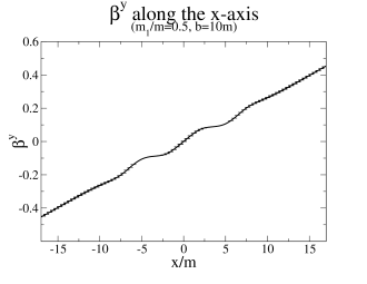
Figure 14: This figure shows the global shift vector along the x-axis with the transition function.

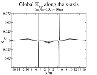
Figure 15: This figure shows the global $xy$ component of the extrinsic curvature along the x-axis with the transition function. Note that the bumps due to the transition function are comparable to the error bars which estimate uncontrolled remainders in the expansions.

We also could have computed the extrinsic curvature directly from Eq. (53). This would add terms involving derivatives of the transition functions. The parameters of the transition functions were chosen so that these derivatives are of the same order as the uncontrolled remainders in the buffer zone, and thus formally do not affect the accuracy of the extrinsic curvature. Since the two methods are equivalent, we took the one which was simpler to compute (had fewer terms).

The initial data constructed by the methods above [Eqs. (53) and (76)] is only an approximate solution to the Einstein equations. Therefore, this data leads to an error in the constraints of the full theory of order $O(m/b)^{9/2}$ near the horizons and $O(m/r)^{2}$ in the near zone. This error can be sufficiently small compared to other sources of numerical error such that solving the constraints more accurately is not required. However, perhaps the optimal approach would be to use this solution as input to York’s conformal method Cook (2000) and compute a numerical solution to the full constraints. Since this data is already significantly close to the constraint hypersurface, there might be some hope that appropriate projection methods will not alter much the astrophysical content of the initial data. Somewhat surprisingly, standard PN data (without matching) has not yet been used for the generation of numerical black hole initial data except in Ref. Tichy et al. (2003a), which is based on the PN data of Ref. Jaranowski and Schafer (1998). We leave it to future work to explore similar techniques for the data set presented here.

If this data is to be evolved, it is necessary to choose a lapse and a shift. The choice presented in this section is natural in the sense that it is close to quasi-equilibrium. In other words, with the lapse and shift presented in this section, the $3$-metric and extrinsic curvature should evolve slowly. However, since our lapse is not everywhere positive, some evolution codes may have trouble evolving with it. If this is the case, one can simply replace the above lapse with a positive function at the cost of losing manifest quasi-equilibrium, but without changing the physical content of the initial data or the results of the evolution.

VIII Conclusions

We have constructed initial data for binary black hole evolutions by calculating a uniform global approximation to the spacetime via asymptotic matching of locally good approximations. The manifold was first divided into three submanifolds: two inner zones (one for each hole), ${\cal{C}}_{1}$ and ${\cal{C}}_{2}$ ($r_{A}\ll b$) equipped with isotropic coordinates; and one near zone, ${\cal{C}}_{3}$ ($r_{A}\gg m_{A}$ and $r\ll\lambda/2\pi$), equipped with harmonic coordinates. In the near zone, the metric was approximated with a post-Newtonian expansion, while in each inner zone the metric was approximated with a perturbative tidal expansion of Schwarzschild geometry. Each approximate solution depends on small parameters locally defined on each submanifold. These submanifolds overlap in two buffer zones, ${\cal{O}}_{13}$ and ${\cal{O}}_{23}$ ($4-$volumes), given by the intersection of the inner zones with the near zone, i.e. on an initial spatial hypersurface the buffer zones becomes $3$-volumes given by $m_{A}\ll r_{A}\ll b$. Inside each buffer zone, two different approximations for the metric were simultaneously valid and hence we were allowed to asymptotically match them inside this zone.

The matching procedure consisted of first expanding both adjacent approximate metrics asymptotically inside the buffer zones. After transforming to the same gauge, these asymptotic expansions were then set asymptotic to each other—equating their expansion coefficients, which does not in general set the functions equal to each other anywhere in the buffer zone. After solving the differential systems given by equating expansion coefficients, asymptotic matching returned a coordinate transformation ($\phi_{13}$ and $\phi_{23}$) between submanifolds and matching conditions ($\psi_{13}$ and $\psi_{23}$) that relate parameters native to different charts. A piecewise global metric was then obtained by transforming all metrics with the set $\left\{\phi_{nm};\psi_{nm}\right\}$, resulting in coordinates which resemble harmonic coordinates in the near zone but isotropic coordinates in each inner zone.

Once a piecewise global metric was found, the spatial metric and extrinsic curvature were calculated in each zone by choosing a spatial hypersurface, with the standard $3+1$ decomposition. This initial data was then transformed in the same manner as the $4$ metric. Due to the inherent piecewise nature of asymptotic matching, this data was found to have discontinuities of order $O(3/2,3)$ or smaller inside the buffer zone. We constructed transition functions to remove the remaining discontinuities in metric components and spikes in derivatives. These transition functions were carefully built to avoid introducing errors larger than the uncontrolled remainders of the approximations in the buffer zones. With these functions, we constructed a global uniform approximation to the metric valid everywhere in the manifold with errors $O(m/b)^{9/2}$ near the black holes and $O(m/r)^{2}$ far away from either of them.

This uniform global approximation of the metric can be used as long as the black holes are sufficiently far apart. When the two black holes are too close, there is no intervening post-Newtonian near zone in which to match. However, since there is no precise knowledge of the region of convergence of the PN series, it is unknown precisely at what separation the near zone vanishes. We have experimented with separations $b\geq 10m$ and we have found that, in these cases, a region does exist between the holes where the post-Newtonian metric is reasonably close to the perturbed black hole metrics and thus matching is still possible. For separations of $b<10m$, this region shrinks rapidly and matching is not guaranteed to be successful. Also, the “global” metric is not valid all the way to the asymptotically flat ends inside the holes, implying that our initial data must be evolved with excision techniques rather than punctures.

We then constructed a lapse, shift, and extrinsic curvature, all of which are needed for numerical evolutions. The lapse was found to possess the expected feature that it becomes negative inside the horizon of either black hole. Some numerical codes might find this feature undesirable, in which case the lapse can be replaced by some positive function at the cost of losing approximate quasi-stationarity. These $3+1$ quantities were then smoothed with transition functions of the same type as those used in the $4$-metric.

In conclusion, we have constructed initial data for an inspiraling black hole binary that satisfies the constraints to order $O[(m/b)^{5/2}(R_{1}/b)^{2}]$ in the inner zone, and to order $O(m/r)^{2}$ in the near zone. This data is a concrete step toward using PN and perturbation methods to construct such initial data, and it should be compared to other numerical methods with respect to its ability to approximate the astrophysical situation. We should note that the data presented here makes use of perturbative expansions of low order (e.g., the near zone metric is built from a $1$ PN expansion), but this paper firms up a method introduced by Alvi Alvi (2000) that could be repeated to higher order at the cost of more algebra Yunes and Tichy (2006a); Yunes and Tichy (2006b). The post-Newtonian metric needed for the next order in $m/r$ (and beyond) is available Blanchet et al. (1998), as is the octopole perturbation $(r/b)^{3}$ of a Schwarzschild black hole Poisson (2005). Our method might also be extended to spinning black holes, which are more astrophysically realistic, with the available post-Newtonian near-zone metric Tagoshi et al. (2001) and tidal perturbation Yunes and Gonzalez (2006).

References

Baumgarte and Shapiro (2003)
T. W. Baumgarte
and S. L.
Shapiro, Phys. Rept.
376, 41 (2003),
and references therein, eprint gr-qc/0211028.
Cook (1994)
G. B. Cook,
Phys. Rev. D 50,
5025 (1994).
Matzner et al. (1999)
R. A. Matzner,
M. F. Huq, and
D. Shoemaker,
Phys. Rev. D 59,
024015 (1999).
Baumgarte (2000)
T. W. Baumgarte,
Phys. Rev. D 62,
024018 (2000), eprint gr-qc/0004050.
Marronetti and Matzner (2000)
P. Marronetti and
R. A. Matzner,
Phys. Rev. Lett. 85,
5500 (2000), gr-qc/0009044.
Cook (2000)
G. B. Cook,
Living Rev. Rel. 3,
5 (2000), and references
therein, eprint gr-qc/0007085.
Grandclément
et al. (2002)
P. Grandclément,
E. Gourgoulhon,
and
S. Bonazzola,
Phys. Rev. D 65,
044021 (2002), eprint gr-qc/0106016.
Pfeiffer et al. (2002)
H. P. Pfeiffer,
G. B. Cook, and
S. A. Teukolsky,
Phys. Rev. D66,
024047 (2002), eprint gr-qc/0203085.
Baker (2002)
B. D. Baker
(2002), eprint [http://arXiv.org/abs]gr-qc/0205082.
Tichy et al. (2003a)
W. Tichy,
B. Brügmann,
M. Campanelli,
and P. Diener,
Phys. Rev. D67,
064008 (2003a),
eprint gr-qc/0207011.
Tichy et al. (2003b)
W. Tichy,
B. Brügmann,
and P. Laguna,
Phys. Rev. D 68,
064008 (2003b),
eprint gr-qc/0306020.
Tichy and Brügmann (2004)
W. Tichy and
B. Brügmann,
Phys. Rev. D 69,
024006 (2004), eprint gr-qc/0307027.
Yo et al. (2004)
H.-J. Yo,
J. N. Cook,
S. L. Shapiro,
and T. W.
Baumgarte, Phys. Rev. D
70, 084033
(2004), eprint gr-qc/0406020.
Cook and Pfeiffer (2004)
G. B. Cook and
H. P. Pfeiffer
(2004), gr-qc/0407078.
Blanchet (2006)
L. Blanchet,
Living Rev. Rel. 9,
4 (2006), and references
therein, eprint gr-qc/0202016.
Yunes and Tichy (2006a)
N. Yunes and
W. Tichy,
Phys. Rev. D74,
064013 (2006a),
eprint gr-qc/0601046.
Yunes and
Tichy (2006b)
N. Yunes and
W. Tichy
(2006b), in progress.
Thorne and Hartle (1985)
K. S. Thorne and
J. B. Hartle,
Phys. Rev. D31,
1815 (1985).
Bender and Orszag (1999)
C. M. Bender and
S. A. Orszag,
Advanced mathematical methods for scientists and
engineers 1, Asymptotic methods and perturbation theory
(Springer, New York,
1999).
Blanchet et al. (2004)
L. Blanchet,
T. Damour,
G. Esposito-Farese,
and B. R. Iyer,
Phys. Rev. Lett. 93,
091101 (2004), eprint gr-qc/0406012.
Poisson (2005)
E. Poisson,
Phys. Rev. Lett. 94,
161103 (2005), eprint gr-qc/0501032.
Will and Wiseman (1996)
C. M. Will and
A. G. Wiseman,
Phys. Rev. D54,
4813 (1996), eprint gr-qc/9608012.
Burke and Thorne (1970)
W. L. Burke and
K. S. Thorne, in
Relativity, edited by
M. Carmeli,
S. I. Fickler,
and L. Witten
(Plenum Press, 1970), pp.
209–228.
Burke (1971)
W. L. Burke,
J. Math. Phys. 12,
401 (1971).
D’Eath (1975a)
P. D. D’Eath,
Phys. Rev. D12,
2183 (1975a).
D’Eath (1975b)
P. D. D’Eath,
Phys. Rev. D11,
1387 (1975b).
Tagoshi et al. (2001)
H. Tagoshi,
A. Ohashi, and
B. J. Owen,
Phys. Rev. D63,
044006 (2001), eprint gr-qc/0010014.
Blanchet et al. (1998)
L. Blanchet,
G. Faye, and
B. Ponsot,
Phys. Rev. D58,
124002 (1998), eprint gr-qc/9804079.
Visser and Yunes (2003)
M. Visser and
N. Yunes,
Int. J. Mod. Phys. A18,
3433 (2003), eprint gr-qc/0211001.
Jaranowski and Schafer (1998)
P. Jaranowski and
G. Schafer,
Phys. Rev. D57,
7274 (1998), eprint gr-qc/9712075.
Yunes and Gonzalez (2006)
N. Yunes and
J. A. Gonzalez,
Phys. Rev. D73,
024010 (2006), eprint gr-qc/0510076.