Hoop Conjecture in Five-dimensions
-Violation of Cosmic Censorship-

Abstract

We study the condition of black hole formation in five-dimensional space-time. We analytically solve the constraint equations of five-dimensional Einstein equations for momentarily static and conformally flat initial data of a spheroidal mass. We numerically search for an apparent horizon in various initial hypersurfaces and find both necessary and sufficient conditions for the horizon formation in terms of inequalities relating a geometric quantity and a mass defined in an appropriate manner. In the case of infinitely thin spheroid, our results suggest a possibility of naked singularity formation by the spindle gravitational collapse in five-dimensional space-time.

I Introduction

In an attempt to unify fundamental forces including gravity, the possibility that the space-time dimensions of our universe is higher than four has been much discussed. Such higher-dimensional theories need mechanism to reduce the space-time dimensions down to four, for example via Kaluza-Klein type compactifications of extra dimensions, so as to be consistent with the observed world. The brane world scenario is another attractive idea of dimensional reduction. In this scenario, the standard model particles are confined to the boundary of a higher-dimensional space-time and only gravity can propagate in the extra dimensions. Models of the brane world scenario with large extra dimensions compared to the four-dimensional Planck scale ($\approx 1.6\times 10^{-33}$cm) have been considered in some recent works BRANE . According to these models, the fundamental (namely, higher-dimensional) Planck scale may be set to rather low energy scale, even to $1$TeV, of which low energy effects just alter the short distance behaviour of classical gravitational interactions. The discrepancy in the gravitational interaction between the four and higher-dimensional theories arises only at the length scale below $0.1{\rm mm}$ so that it is consistent with the gravitational experiments experiments . In such TeV gravity models, it is suggested that small black holes are produced in accelerators, such as the CERN Large Hadron Collider LHC or in high energy cosmic ray events Feng:2001ib .

In order to understand physical phenomena caused by strong gravitational fields, the criterion for black hole formation is very crucial. In the case of four-dimensional Einstein gravity, such a criterion is well known as the hoop conjecture HC . Hoop conjecture claims that the necessary and sufficient condition for black hole formation is given by the following; Black holes with horizons form when and only when a mass $M$ gets compacted into a region whose circumference in every direction is ${\cal C}\lesssim 4\pi G_{4}M$, where $G_{4}$ is the gravitational constant in four-dimensional theory of gravity. It is remarkable that no serious counterexample against hoop conjecture has been presented. However, at first glance, hoop conjecture is not valid in higher-dimensional Einstein gravity Nakao:2001pn ; there is black string solutions in five or higher-dimensions, which have infinitely long event horizons, while hoop conjecture claims that any length scale characterizing black hole should be less than the gravitational length scale determined by the Schwarzschild radius.

Recently, two of the present authors, DI and KN, proposed a higher-dimensional version of hoop conjecture IN . Here we call it the hyperhoop conjecture in the sense that it is a possible generalization of the original hoop conjecture; Black holes with horizons form when and only when a mass $M$ gets compacted into a region whose $(D-3)$-dimensional area $V_{D-3}$ in every direction is

$$V_{D-3}\lesssim G_{D}M,$$ (1)

where $G_{D}$ is the gravitational constant in $D$-dimensional theory of gravity, and the ($D-3$)-dimensional area means the volume of $(D-3)$-dimensional closed submanifold of a spacelike hypersurface. Hereafter we call this $(D-3)$-dimensional closed submanifold the hyperhoop. The necessity of the condition (1) was confirmed in the case of momentarily static and conformally flat initial data sets of an axially symmetric line, disk and thin ring source for the five-dimensional Einstein equations IN and for the system of point-particles Yoshino:2002tx . Consistent results with the previous ones were obtained by Barrabés et al BFL . They derived two inequalities for ($D-3$)-dimensional volume as the necessary and sufficient conditions for apparent horizon formation in the case of a ($D-2$)-dimensional convex thin shell collapsing with the speed of light in a $D$-dimensional space-time.

The purpose of the present paper is to study both the necessity and in particular sufficiency of the inequality (1) for the horizon formation in different situations from the case treated in Ref. BFL . We consider the momentarily static and conformally flat four-dimensional initial hypersurfaces in which a four-dimensional homogeneous spheroid is put as a gravitational source. This procedure has been implemented by Nakamura et al. Nakamura:1988zq . We apply their method to higher-dimensional case. Then, we analytically solve the constraint equations for five-dimensional Einstein equations. In order to investigate the validity of hyperhoop conjecture, we numerically search for an apparent horizon and calculate the ratio $V_{2}/G_{5}M$ for substantially various hyperhoops.

This paper is organized as follows. In Sec. II, assuming five-dimensional Einstein gravity, we derive the constraint equations for conformally flat initial hypersurfaces and then give analytic solutions of these equations for a homogeneous mass of a spheroidal shape. In Sec. III, we search for an apparent horizon in initial hypersurfaces with various shapes of a homogeneous spheroid including infinitely thin case by numerically solving a second order ordinary differential equation. This equation corresponds to the minimum volume condition for a three-dimensional closed submanifold of an initial hypersurface. The suggestion of the naked singularity formation is given in this section. In Sec. IV, we define $V_{2}/G_{5}M$ in a reasonable manner and then give a procedure to select the hyperhoop with minimal value of $V_{2}/G_{5}M$. In Sec. V, we show numerical results and their implication to the necessary and sufficient condition for the horizon formation. Finally, Sec. VI is devoted to summary. In Appendix A, we derive analytic solutions for the Newtonian gravitational potential of an ellipsoid in arbitrary space dimension. In Appendix B, the necessary condition of black hole formation based on Ref.IN is derived.

In this paper, we adopt the unit of $c=1$. We basically follow the notations and sign conventions in Ref.Wald .

II A Momentarily static spheroid in five-dimensional space-time

Let us consider an initial data set $\left(h_{ab},K_{ab}\right)$ in a four-dimensional spacelike hypersurface $\Sigma$, where $h_{ab}$ is the induced metric in $\Sigma$ and $K_{ab}$ is the extrinsic curvature which represents how $\Sigma$ is embedded in the five-dimensional space-time. Denoting the unit normal vector to $\Sigma$ by $n^{a}$, $h_{ab}$ and $K_{ab}$ are, respectively, written as

$$h_{ab} = g_{ab}+n_{a}n_{b},$$ (2)

$$K_{ab} = -h_{a}^{c}\nabla_{c}n_{b},$$ (3)

where $\nabla_{c}$ is the covariant derivative in the five-dimensional space-time.

The initial data set $(h_{ab},K_{ab})$ has to satisfy the Hamiltonian and momentum constraints given by

$${\cal R}-K_{ab}K^{ab}+K^{2}=24\pi^{2}G_{5}\rho$$ (4)

and

$$D_{b}\left(K^{ab}-h^{ab}K\right)=12\pi^{2}G_{5}J^{a},$$ (5)

where $\rho$ and $J^{a}$ are the energy density and energy flux for normal line observers to $\Sigma$, $D_{a}$ and ${\cal R}$ are the covariant derivative within $\Sigma$ and the scalar curvature of $h_{ab}$, and $G_{5}$ is the gravitational constant in five-dimensional theory of gravity. In this paper, we focus on momentarily static and conformally flat initial hypersurfaces:

$$K_{ab} = 0$$ (6)

$$h_{ab} = f^{2}\delta_{ab},$$ (7)

where $\delta_{ab}$ is the metric tensor of four-dimensional Euclidean space. We also require the axial symmetry in the sense that the metric on $\Sigma$ have the form

$$dl^{2}=f^{2}(R,z)\left[dR^{2}+R^{2}\left(d\vartheta^{2}+\sin^{2}\vartheta d\varphi^{2}\right)+dz^{2}\right],$$ (8)

where $0\leq R<+\infty$ and $-\infty<z<+\infty$ while $\vartheta$ and $\varphi$ are the round coordinates. Then the momentum constraint leads to zero flux condition $J^{a}=0$, and the Hamiltonian constraint becomes

$${\partial^{2}f\over\partial R^{2}}+{2\over R}{\partial f\over\partial R}+{\partial^{2}f\over\partial z^{2}}=-4\pi^{2}G_{5}f^{3}\rho.$$ (9)

Here we note that the Hamiltonian constraint (9) is equivalent to the Poisson equation for axi-symmetric Newtonian gravitational potential. Let us consider the density profile respecting the axial symmetry given by

$$f^{3}\rho=\left\{\begin{array}[]{lll}2M/\pi^{2}a^{3}b&\mbox{for}&R^{2}/a^{2}+z^{2}/b^{2}{\leq}1,\\ ~{}~{}~{}~{}0&\mbox{for}&\mbox{elsewhere},\end{array}\right.$$ (10)

where $a$, $b$ and $M$ are constant parameters.

We consider the gravitational field of an isolated body, so that we assume the asymptotic condition given by

$$f\rightarrow 1~{}~{}~{}{\rm for}~{}~{}r\rightarrow\infty,$$ (11)

where

$$r=\sqrt{R^{2}+z^{2}}.$$ (12)

The regular solution is then obtained as

$$f = 1-\frac{4G_{5}M\left[b(2a+b)R^{2}+3a^{2}z^{2}-3a^{2}b(a+b)\right]}{3a^{3}b{\left(a+b\right)}^{2}}$$ (13)

$$~{}~{}~{}~{}~{}~{}~{}~{}~{}~{}~{}~{}~{}~{}~{}~{}~{}~{}~{}~{}~{}~{}~{}~{}~{}~{}~{}~{}~{}~{}~{}~{}~{}~{}{\rm for}~{}~{}\frac{R^{2}}{a^{2}}+\frac{z^{2}}{b^{2}}~{}{\leq}~{}1,$$

$$f = 1-\frac{4G_{5}M}{3e^{4}b^{4}}\Biggl{[}2R^{2}-6z^{2}+3e^{2}b^{2}+\sqrt{F^{2}-e^{4}b^{4}}$$ (14)

$$\times \biggl{(}{2e^{2}b^{2}R^{2}\over(F-e^{2}b^{2})^{2}}-{2R^{2}-3z^{2}+3e^{2}b^{2}\over F-e^{2}b^{2}}+{3z^{2}\over F+e^{2}b^{2}}\biggr{)}\Biggr{]}$$

$$~{}~{}~{}~{}~{}~{}~{}~{}~{}~{}~{}~{}~{}~{}~{}~{}~{}~{}~{}~{}~{}~{}~{}~{}~{}~{}~{}~{}~{}~{}~{}~{}~{}~{}{\rm for}~{}~{}\frac{R^{2}}{a^{2}}+\frac{z^{2}}{b^{2}}>1,$$

where $e$ is the eccentricity defined by

$$e=\sqrt{1-{a^{2}\over b^{2}}}$$ (15)

and $F$ is a function of $R$ and $z$ defined by

$$F = F(R,z;a,b)$$

$$= R^{2}+z^{2}+\sqrt{4b^{2}R^{2}-4a^{2}\left(b^{2}-z^{2}\right)+{\left(a^{2}+b^{2}-R^{2}-z^{2}\right)}^{2}}.$$

The detailed derivation of the above solution is given in Appendix A. Newtonian gravitational potential of an ellipsoid in Euclidean space of arbitrary dimensions is shown there. Here we only investigate the prolate case $a<b$.

In the thin limit $a\rightarrow 0$ with $M$ and $b$ fixed, two disconnected singularities appear at the poles $(R,z)=(0,\pm b)$ of the resultant “singular spheroid”. In order to see this, we evaluate the Kretschmann invariant

$$I={\cal R}^{abcd}{\cal R}_{abcd},$$ (17)

where ${\cal R}_{abcd}$ is the four-dimensional Riemann tensor of the spacelike hypersurface. Typical examples are shown in Figs. 1 and 2. The coordinate values and the Kretschmann invariant $I$ is normalized by

$$r_{\rm s}:=\sqrt{G_{5}M}.$$ (18)

It will be found in the next section that $r_{\rm s}$ is the coordinate radius of the apparent horizon in the case of a point source $a=b=0$.

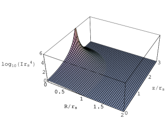
Figure 1: The logarithm to the base 10 of the Kretschmann invariant $I$ is plotted as function of the coordinates $R$ and $z$ in the case $a=0$ and $b=2r_{\rm s}$.

Figure 2: The logarithm to the base 10 of the Kretschmann invariant $I$ on the polar axis $(R=0)$ is plotted as function of $z$ in the case $a=0$ and $b=2r_{\rm s}$. The value of $I$ is diverge at only $(0,b)$.

Here it should be noted that the Kretschmann invariant $I$ is finite between these two singularities on the singular spheroid, $R=0$ and $|z|<b$. Further, we can see that the energy density $\rho$ is also finite there. The conformal factor on the surface of the spheroid is given by

$$f = f_{\rm sf}(z)$$ (19)

$$:= 1+{4G_{5}M\over 3ab^{2}(a+b)^{2}}\left[b^{2}(a+2b)-2(b-a)z^{2}\right].~{}~{}$$

Therefore we find that the energy density at the surface becomes in the thin limit $a\rightarrow 0$ as

$$\rho=\rho_{\rm sf}(z):={2M\over\pi^{2}a^{3}bf_{\rm sf}^{3}}\longrightarrow{27b^{8}\over 256\pi^{2}G_{5}^{3}M^{2}(b^{2}-z^{2})^{3}}.$$ (20)

Here note that the inequality $f(R,z)\geq f_{\rm sf}(z)$ is satisfied within the spheroid and hence $0\leq\rho(R,z)\leq\rho_{\rm sf}(z)$. Therefore $\rho$ is finite except for the poles $z=\pm b$ even in the thin limit $a\rightarrow 0$. This fact means that the scalar polynomials of the five-dimensional Riemann tensor are also finite if the stress of matter fields is assumed to be reasonable. For example, assuming the dust as the matter and adopting Gaussian normal coordinate, Einstein equations leads to

$${\partial K^{a}{}_{b}\over\partial t}={\cal R}^{a}{}_{b}-4\pi^{2}G_{5}\rho~{}\delta^{a}{}_{b}$$ (21)

on the momentarily static initial hypersurface, where ${\cal R}^{a}{}_{b}$ is the four-dimensional Ricci tensor of this hypersurface. Here note that ${\cal R}^{a}{}_{b}$ is finite in the region of finite Kretschmann invariant $I$ since the metric of the spacelike hypersurface is positive definite. Therefore the finiteness of the energy density $\rho$ guarantees that the time derivative of the extrinsic curvature $K^{a}{}_{b}$ is finite in the region of finite Kretschmann invariant $I$. This means that the scalar polynomials of Riemann tensor of five-dimensional space-time are also everywhere finite except for the poles of the singular spheroid since these are expressed as polynomials of $\partial K^{a}{}_{b}/\partial t$, ${\cal R}^{a}{}_{b}$, $K^{a}{}_{b}$ and $D_{c}K^{a}{}_{b}$ in the Gaussian normal coordinate. Further, we can see that this singular spheroid except for the poles corresponds to spatial infinity. Consider a curve $z=\zeta(R)$ connecting two points $R=R_{1}$ and $R=R_{2}$ ($R_{1}<R_{2}$) and assume that both $R_{1}$ and $R_{2}$ are sufficiently small and $0<\zeta(R)<z_{\rm max}<b$. In this situation, the function $F$ is written as

$$F(R,\zeta;0,b)=b^{2}+\frac{2b^{2}}{b^{2}-\zeta^{2}}R^{2}+\mathcal{O}(R^{3}).$$ (22)

Hence substituting this for Eq. (14), we find

$$f\left(R,\zeta\right)={8(b^{2}-\zeta^{2})^{3/2}G_{5}M\over 3b^{4}R}+\mathcal{O}(R^{0}).$$ (23)

The proper length between $R=R_{1}$ and $R_{2}$ along the curve $z=\zeta(R)$ is bounded below as

$$\int_{R_{1}}^{R_{2}}f(R,\zeta)\sqrt{1+\left({d\zeta\over dR}\right)^{2}}~{}dR$$

$$\geq\int_{R_{1}}^{R_{2}}f(R,\zeta)dR\simeq{8G_{5}M\over 3b^{4}}\int_{R_{1}}^{R_{2}}(b^{2}-\zeta^{2})^{3/2}{dR\over R}$$

$$\geq{8G_{5}M\over 3b^{4}}(b^{2}-z_{\rm max}^{2})^{3/2}\int_{R_{1}}^{R_{2}}{dR\over R}={8G_{5}M\over 3b^{4}}(b^{2}-z_{\rm max}^{2})^{3/2}\ln{R_{2}\over R_{1}}.$$ (24)

We can see from the above equation that the proper length diverges in the limit of $R_{1}\rightarrow 0$ with $R_{2}$ fixed. Therefore each point on the singular spheroid except for the poles, $R=0$ and $|z|<b$, is spacelike infinity.

III Apparent horizons

In a momentarily static initial hypersurface in five-dimensional asymptotically flat space-time, an apparent horizon is a three-dimensional closed marginal surface. Because of the axial symmetry of the initial hypersurface, the apparent horizon will also be axially symmetric and thus will be expressed by $r=r_{\rm m}(\xi)$ in the present case, where

$$\xi=\arctan{R\over z}.$$ (25)

Then $r=r_{\rm m}(\xi)$ is a closed marginal surface only if $r_{\rm m}(\xi)$ satisfies

$${\ddot{r}}_{\rm m}-{4{\dot{r}}_{\rm m}{}^{2}\over r_{\rm m}}-3r_{\rm m}+\frac{r_{\rm m}{}^{2}+{\dot{r}}_{\rm m}{}^{2}}{r_{\rm m}}$$

$$\times\left[\frac{2{\dot{r}}_{\rm m}}{r_{\rm m}}\cot\xi-{3\over f}\left({\dot{r}}_{\rm m}\sin\xi+r_{\rm m}\cos\xi\right)\frac{\partial f}{\partial z}+{3\over f}\left({\dot{r}}_{\rm m}\cos\xi-r_{\rm m}\sin\xi\right)\frac{\partial f}{\partial R}\right]=0$$ (26)

with boundary conditions ${\dot{r}}_{\rm m}=0$ at $\xi=0$ and $\pi$, where a dot means the derivative with respect to $\xi$. The derivation of Eq. (26) is shown in Appendix C. Since the present system has a reflection symmetry with respect to $z=0$, the apparent horizon should satisfy

$${\dot{r}}_{\rm m}=0~{}~{}{\rm at}~{}~{}{\xi=\frac{\pi}{2}}.$$ (27)

In the case of a point source $a=b=0$, we can analytically solve Eq. (26) and find

$$r_{\rm m}=r_{\rm s}.$$ (28)

Replacing derivatives with respect to $\xi$ in Eq. (26) by finite differences, we numerically search for solutions of this equation by relaxation method ref:SMMN . If apparent horizons exist in the initial hypersurface, we can find solutions of Eq. (26). Typical examples are shown in Fig. 3. The coordinate values are normalized by $r_{\rm s}$.

Figure 3: Apparent horizons for each shape of the four-dimensional spheroid are depicted in $(R,z)$-plane. The solid line shows the surface of the spheroid. The dashed line shows the apparent horizon if it is present.

In the case of singular source $a=0$, we also find solutions of Eq. (26) satisfying the boundary condition (27). In the case of $b\leq 1.48r_{\rm s}$, there is an apparent horizon enclosing whole the singular source. By contrast, for $b\geq 1.49r_{\rm s}$, the marginal surface covers only a central part of the singular source, and the space-time singularities at the poles $(R,z)=(0,\pm b)$ are not enclosed by the marginal surface (see Fig. 4). In this case, this marginal surface is not a closed three-surface and thus is not the apparent horizon since as mentioned in the previous section, $|z|<b$ on the polar axis $R=0$ is the spacelike infinity. This result implies that a long enough spindle singular source can produce naked singularities, which is quite different from the singular line source in Ref. IN .

Figure 4: In the case of $a=0$, apparent horizons for each $b$ are depicted.

IV How to check hyperhoop conjecture

We have presented the statement of hyperhoop conjecture in Sec. I. Here we should note that in general, the mass $M$ in hyperhoop conjecture (and also in hoop conjecture) is not the total mass of the system but the mass encircled by the hyperhoop (the hoop). Therefore to check the sufficiency of this conjecture, we have to confirm that in an initial hypersurface without an apparent horizon, there is no hyperhoop satisfying

$$V_{D-3}\lesssim G_{D}M_{\rm in},$$ (29)

where $M_{\rm in}$ is not the total mass of the system but the one included in the region which is encircled by this hyperhoop.

Since we cannot try all the possible hyperhoops in $\Sigma$, we focus on the axi-symmetric hyperhoops which have the reflection symmetry with respect to $z=0$. Further, these hyperhoops are expressed in the form $r=r_{\rm h}(\xi)$ and $\vartheta=\pi/2$ since the spheroid is assumed to be prolate $a<b$.(In the oblate case, we should consider two-surface of $z=0$ and $R=$constant, where the hyperhoop is parameterized by two parameters $\xi$ and $\varphi$.) The two-dimensional area $V_{2}$ of the hyperhoop $r=r_{\rm h}(\xi)$ and $\vartheta=\pi/2$ is then given by

$$V_{2}=\int_{0}^{2\pi}d\varphi\int^{\pi}_{0}d\xi f^{2}\sqrt{{\dot{r}}_{\rm h}{}^{2}+r_{\rm h}{}^{2}}~{}r_{\rm h}\sin\xi=4\pi\int^{\pi/2}_{0}d\xi f^{2}\sqrt{{\dot{r}}_{\rm h}{}^{2}+r_{\rm h}{}^{2}}~{}r_{\rm h}\sin\xi,$$ (30)

where we have taken account of the reflection symmetry in the second equality.

In the framework of general relativity, there is no unique definition of the mass in a quasilocal manner although the total mass is well defined for the isolated system. This is one of reasons why it is very difficult to formulate precisely the hoop and also hyperhoop conjectures. However, despite of this mathematical indefiniteness, the hoop and hyperhoop conjectures might be useful in understanding black hole formation processes on the physical ground. In this sense, all the reasonable definitions of quasilocal mass will be meaningful in the hoop and hyperhoop conjectures since these might give the results not so different from each other. Here we adopt the following simple definition for the mass $M_{\rm in}$ as

$$M_{\rm in}=8\pi\int^{\pi/2}_{0}d\xi\int^{r_{\rm h}\left(\xi\right)}_{0}dr\rho f^{3}r^{3}\sin^{2}\xi.$$ (31)

Then we numerically calculate $V_{2}/G_{5}M_{\rm in}$ for various hyperhoops in an initial hypersurface of a spheroid. Hereafter for notational simplicity, we introduce

$$\Gamma:={V_{2}\over 16\pi G_{5}M_{\rm in}},$$ (32)

where $16\pi G_{5}M_{\rm in}$ is the minimal value of $V_{2}$ in the case of a point source whose mass is $M_{\rm in}$.

Our first task is the selection of relevant hyperhoops from all the possible hyperhoops expressed by $r=r_{h}(\xi)$ and $\vartheta=\pi/2$ with the reflection symmetry with respect to $z=0$. A hyperhoop is represented as a continuous curve from a point on $z$-axis to a point on $R$-axis in the first quadrant of $(R,z)$-plane. Thus first, we select a point $z=z_{0}$ on $z$-axis and consider various hyperhoops which start from this point. Since the spheroid of the mass is assumed to be prolate, we expect that the significant hyperhoops are also prolate, and thus we restrict the curves within the region of $R^{2}+z^{2}\leq z_{0}^{2}$. The number of possible curves is still infinite. Therefore we impose further restrictions. Consider 100 points $\left(R,z\right)=\left(R^{(1)}_{j_{i}}(z_{0}),z_{i}(z_{0})\right)$ $(i,j_{i}=1,2,..,10)$ within this spherical region; $z_{i}(z_{0})$ is determined in the following manner

$$z_{i}(z_{0})={z_{0}\over 10}(10-i),$$ (33)

and then $R_{j_{i}}^{(1)}(z_{0})$ is given as

$$R^{(1)}_{j_{i}}(z_{0})={\sqrt{z_{0}{}^{2}-z_{i}{}^{2}(z_{0})}\over 10}j_{i}.$$ (34)

We consider the curves composed of ten straight lines connected at $(R,z)=\left(R^{(1)}_{j_{i}}(z_{0}),z_{i}(z_{0})\right)$; $i$ is in order from $1$ to $10$, and then for each $i$, $j_{i}$ is appropriately chosen among ten integers from 1 to 10.

By investigating several randomly chosen hyperhoops, we found that sharply bended one might have a value of $\Gamma$ larger than the ones not so sharply bended. Hence in the systematic numerical search, a line from the point of $(R,z)=\left(R^{(1)}_{j_{i}}(z_{0}),z_{i}(z_{0})\right)$ to $(R,z)=\left(R^{(1)}_{j_{i+1}}(z_{0}),z_{i+1}(z_{0})\right)$ is adopted as a constitutive one of the hyperhoop only if $j_{i+1}$ is equal to $j_{i}$ or $j_{i}\pm 1$ for $j_{i}>1$ and is equal to $j_{i}$ or $j_{i}+1$ for $j_{i}=1$. All the possible constitutive lines are depicted in Fig. 5. This means that we consider only the hyperhoops each of which is a connected set of ten constitutive lines. Then we calculate $\Gamma$ for each hyperhoop and search for the minimal one which is specified by a set of ten integers $\{m_{i}\}$ in the manner of $j_{i}=m_{i}$. Further for several values of $z_{0}$, we carry out the same calculations as the above. We select the values of $z_{0}$ at even intervals $0.1r_{s}$ and search for the hyperhoop with the smallest value of $\Gamma$. Finally, we obtain the minimal one which is specified by a set of ten integers and one real number $\{m_{i},q\}$, where $q$ is the value of $z_{0}$. The above hyperhoop $\{m_{i},q\}$ might not be exactly minimal since the hyperhoops obtained by the above procedure are too restrictive. Thus we might find hyperhoops smaller than the one $\{m_{i},q\}$ in the following refinement. We consider a neighbourhood $R^{(1)}_{m_{i}-1}(q_{0})\leq R\leq R^{(1)}_{m_{i}+1}(q_{0})$ of the hyperhoop $\{m_{i},q_{0}\}$, where $q_{0}$ is a value which is equal or near to $q$. In this region, we put further grid points at

$$R=R^{(2)}_{k_{i}}(q_{0})=R^{(1)}_{m_{i}-1}(q_{0})+{\sqrt{q_{0}^{2}-q_{i}^{2}(q_{0})}\over 50}(k_{i}-1),~{}~{}(k_{i}=1,2,\cdots,11),$$ (35)

where

$$q_{i}(q_{0})=\frac{q_{0}}{10}\times(10-i).$$ (36)

Then by the same procedure as in the previous search for the minimal hyperhoop, we will obtain the hyperhoop with $\Gamma$ smaller than the previous one (see Fig. 6). Further for several value of $q_{0}$ in the vicinity of $q$, we carry out the same calculations as the above. We select the 11 values

$$q-0.1r_{s}+0.02r_{s}(l-1),~{}~{}(l=1,2,\cdots,11)$$ (37)

as $q_{0}$ and search for the hyperhoop with the smallest value of $\Gamma$.

Figure 5: The connecting points (left figure) and the hyperhoops which we calculate for a value of $z_{0}$ (right figure) in first search.

Figure 6: The hyperhoop having the smallest value of $\Gamma$ in first search (left figure) and the hyperhoops which we calculate for a value of $q_{0}$ (right figure) in second search .

V Numerical Results

For various $a$ and $b$, numerical results of the minimal value of $\Gamma$ are listed in TABLE 1. Hereafter we denote the minimal value of $\Gamma$ by $\Gamma_{\rm min}$ which is a function of $a$ and $b$.

We see from TABLE 1 that $\Gamma_{\rm min}$ is not smaller than unity in the case of no apparent horizon. This implies that the inequality (29) is really a sufficient condition in the situations studied here.

Table 1: The minimal values of $\Gamma$ $\left(\Gamma_{\rm min}\right)$ is shown for each $a$ and $b$. The existence of an apparent horizon is represented by (Yes):exist and (No):not exist.

$b\backslash a$	0	0.01	0.1	0.3	0.5	0.7	0.9
1.0	1.05(Yes)	1.05(Yes)	1.05(Yes)	1.05(Yes)	1.04(Yes)	1.03(Yes)	1.01(Yes)
1.5	1.11(No)	1.11(Yes)	1.11(Yes)	1.10(Yes)	1.10(Yes)	1.09(No)	1.08(No)
2.0	1.17(No)	1.17(Yes)	1.17(Yes)	1.17(No)	1.16(No)	1.16(No)	1.17(No)
2.5	1.23(No)	1.23(Yes)	1.23(No)	1.23(No)	1.23(No)	1.24(No)	1.26(No)
3.0	1.29(No)	1.29(Yes)	1.29(No)	1.29(No)	1.30(No)	1.31(No)	1.35(No)
3.5	1.35(No)	1.34(No)	1.34(No)	1.34(No)	1.35(No)	1.38(No)	1.43(No)
4.0	1.40(No)	1.38(No)	1.38(No)	1.38(No)	1.40(No)	1.44(No)	1.51(No)

Next, let us study the necessity of hyperhoop conjecture (29). By the investigation of the singular line source of a “constant” line energy density studied in Ref. IN , we obtain a necessary condition as follows

$$V_{2}\lesssim\frac{\pi}{2}\times 16\pi G_{5}M.$$ (38)

The derivation of this quantity $\pi/2$ is shown in Appendix B. The counterexample for this condition is not found in TABLE 1. Here, it is again noted that a closed marginal surface is formed only when $b\leq 1.48r_{\rm s}$, and thus our result of $a=0$ suggests the formation of naked singularities in the case $b\geq 1.49r_{\rm s}$. If it is true, the naked singularities might form by the gravitational collapse starting from the initial data of nonvanishing but sufficiently small $a$ and $b$ larger than $1.49r_{\rm s}$. If a naked singularity exists, the apparent horizon does not necessarily mean the existence of a black hole. Therefore, although the apparent horizon forms for $a\in[0.01,0.5]$ and $b=1.5r_{\rm s}$ (see TABLE 1), these results do not necessarily mean the black hole formation.

Finally, in the present situation, we find the following inequalities,

$${\rm Necessary~{}condition:}~{}~{}V_{2}\lesssim\frac{\pi}{2}16\pi G_{5}M,$$ (39)

$${\rm Sufficient~{}condition:}~{}~{}V_{2}\lesssim 16\pi G_{5}M.$$ (40)

Our numerical results suggest that the necessary condition is not identical to the sufficient condition.

VI Summary

We have investigated the condition of apparent horizon formation in the case of momentarily static and conformally flat initial data of a spheroidal mass in the framework of five-dimensional Einstein gravity. All our results are consistent with the hyperhoop conjecture. Particularly, we confirmed the sufficiency of the inequality (1). (More precisely, inequality (29) holds in the present case.)

We also consider the limit of infinitely prolate spheroid. The gravitational field of such spheroids are singular and have a nontrivial structure. The poles at the both ends of this singular spheroid are the space-time singularities since the Kretschmann invariant diverges at the poles of the spheroid. On the other hand, both the Kretschmann invariant and the energy density are finite elsewhere.

We find that the singular spheroid is spacelike infinity except for the poles. Furthermore, when the singular spheroid is sufficiently long, in an appropriate sense, no apparent horizon appears. This property can be regarded as being peculiar to nonuniform distribution of material energy, because a uniform line energy density is always enclosed by an apparent horizon in spite of its length IN .

One might wonder if the singular spheroid is a counterexample to the hyperhoop conjecture, since it is infinitely thin and hence there seems to be a hyperhoop satisfying the inequality (1). However as we have shown, the singular spheroid is not a counterexample to the hyperhoop conjecture. In order to understand its reason, we have to note two important features of the initial hypersurface studied here. First, the proper area $V_{2}$ of a hyperhoop tightly encircling the surface of the spheroid is not necessarily smaller than those encircling outside of the spheroid, since the conformal factor in the inner region takes the value larger than that in the outer region. Second, the proper area $V_{2}$ of a hyperhoop tightly encircling the spheroid does not necessarily become smaller when the coordinate size of the spheroid characterized by $a$ and $b$ becomes smaller, since the conformal factor in the spheroid of the smaller size becomes larger if the mass $M$ is fixed.

The difference between the present case and the previous work IN is that the line energy density vanishes continuously at the poles in the present case, while it vanishes discontinuously at the poles in the previous case. In general, if an infinitely thin line object forms by the gravitational collapse, it might have a line energy density which continuously vanishes at the end of the matter distribution. Therefore, the naked singularity formation seems to be generic in the axi-symmetric gravitational collapse of highly elongated matter distribution in five-dimensional space-time, although we would need numerical simulation to have a definite evidence for the naked singularity formation Shapiro:1990 . This might strongly depend on the spacetime dimension Patil:2003yp and this is also a future work.

Appendix A Newtonian potentials of a homogeneous ellipsoid in $D$-dimensional space-time

In this section, we extend Newtonian potentials of a homogeneous ellipsoid in four-dimensional space-time to $(n+1)$-dimensional space-time. The reader may refer to Ref. EFE about the potentials of four-dimensional space-time.

We want to obtain the potentials of the homogeneous ellipsoid of which bounding ellipsoid is

$$\sum^{n}_{i=1}\frac{x_{i}^{2}}{a_{i}^{2}}=1.$$ (41)

At the beginning of derivation, we define the “homoeoid”.

Definition. A $n$-dimensional homoeoid is a shell bounded by two similar concentric $n$-dimensional ellipsoids in which strata of equal density are also $n$-dimensional ellipsoids that are concentric with and similar to the bounding ellipsoids.

Following theorem and corollary is derived in the same way as the case of four-dimensional space-time EFE .

Theorem. The potential at internal point of a $n$-dimensional homoeoid is constant.

Corollary. The equipotential surfaces external to a thin $n$-dimensional homoeoid are $n$-dimensional ellipsoids confocal to the homoeoid.

We can obtain the potential of a thin $n$-dimensional homoeoid expressed as

$$\sum^{n}_{i=1}\frac{x_{i}^{2}}{a_{i}^{2}}=1,~{}~{}(a_{1}<a_{2}<\cdots<a_{n}),$$ (42)

using $n$-dimensional ellipsoidal coordinates $(y_{1},y_{2},\cdots,y_{n})$ which satisfy

$$\sum^{n}_{i=1}\frac{x_{i}^{2}}{a_{i}^{2}-y_{j}}=1,~{}~{}(j=1,2,\cdots,n)$$ (43)

and

$$y_{1}<y_{2}<\cdots<y_{n}.$$ (44)

We can solve Eq. (43) for $x_{i}^{2}$ and

$$x_{i}^{2}=\frac{\prod_{j=1}^{n}(a_{i}^{2}-y_{j})}{\prod_{k\neq i}(a_{i}^{2}-a_{k}^{2})}.$$ (45)

Therefore

$$\frac{\partial x_{i}}{\partial y_{j}}=\frac{x_{i}}{2(y_{j}-a_{i}^{2})}.$$ (46)

The metric is expressed as

$$\sum_{i=1}^{n}dx_{i}^{2}=\frac{1}{4}\sum_{i=1}^{n}\frac{\prod_{k\neq i}(y_{i}-y_{k})}{\prod_{j=1}^{n}(a_{j}^{2}-y_{i})}dy_{i}^{2},$$ (47)

thus

$$\det g=\left(\frac{1}{4}\right)^{n}\frac{\prod_{j=1}^{n}\left[\prod_{k\neq j}(y_{j}-y_{k})\right]}{\prod_{i,j}(a_{i}^{2}-y_{j})}.$$ (48)

In order to obtain the potential $\Phi_{N}$ of a thin $n$-dimensional homoeoid, we only have to solve following equation because of the theorem and the corollary.

$$\triangle\Phi_{N}(y_{1})=0$$ (49)

with

$$\Phi_{N}\rightarrow-\frac{M}{(n-2)r^{n-2}}~{}~{}~{}{\rm for}~{}~{}~{}r\rightarrow\infty,$$ (50)

where $M$ is constant which correspond to the mass of the thin $n$-dimensional homoeoid and $r$ is the length from the center of the homoeoid. It can be seen that $-y_{1}\sim r^{2}$ at infinity. Using ellipsoidal coordinates to Eq. (49), we obtain

$$\frac{\partial}{\partial y_{1}}\left[\prod_{i=1}^{n}\sqrt{a_{i}^{2}-y_{1}}\frac{\partial\Phi_{N}(y_{1})}{\partial y_{1}}\right]=0.$$ (51)

The solution of Eq. (51) with (50) is

$$\Phi_{N}(u)=-\frac{n-2}{2}M\int^{\infty}_{u}\frac{1}{\prod_{i=1}^{n}\sqrt{a_{i}^{2}+u}}du,$$ (52)

where $u=-y_{1}$.

Integrating this potentials of thin homoeoid which is foliated in all region of ellipsoid in the same manner as four-dimensional space-time EFE , we can finally obtain the Newtonian potential of a $D$-dimensional homogeneous ellipsoid. The integration can be done as follows. We can express the thin homoeoids which is similar and concentric to the ellipsoid (41) as

$$\sum^{n}_{i=1}\frac{x_{i}^{2}}{a_{i}^{2}}=m^{2},$$ (53)

where $m$ is constant and we assume $0\leq m\leq 1$. Let us consider the homogeneous homoeoid bounded by two ellipsoids $\sum^{n}_{i=1}\frac{x_{i}^{2}}{a_{i}^{2}}=m^{2}$ and $\sum^{n}_{i=1}\frac{x_{i}^{2}}{a_{i}^{2}}=(m+dm)^{2}$, where $dm$ is small deviation. The mass of this homoeoid is

$$\omega_{n}a_{1}a_{2}\cdots a_{n}\rho m^{n-1}dm,$$ (54)

where $\omega_{n}$ and $\rho$ is $n$-dimensional solid angle and the density of the homoeoid respectively.

First, we derive the potential in outer region of homogeneous ellipsoid. Substituting (54) into $M$ of (52), we can obtain the potential of the homoeoidal element (54) at $(x^{\prime}_{1},x^{\prime}_{2},\cdots,x^{\prime}_{n})$

$$-\frac{n-2}{2}\omega_{n}a_{1}a_{2}\cdots a_{n}\rho m^{n-1}dm\int^{\infty}_{\lambda(m^{2})}\frac{du^{\prime}}{\prod^{n}_{i=1}\sqrt{a_{i}^{2}m^{2}+u^{\prime}}},$$ (55)

where $\lambda$ is the largest root of $\sum^{n}_{i=1}\frac{{x^{\prime}_{i}}^{2}}{m^{2}a_{i}^{2}+\lambda}=1$. Integrating this equation about $0\leq m\leq 1$, we have

$$-\frac{n-2}{2}\omega_{n}a_{1}a_{2}\cdots a_{n}\rho\int^{1}_{0}dmm^{n-1}\int^{\infty}_{\lambda(m^{2})}\frac{du^{\prime}}{\prod^{n}_{i=1}\sqrt{a_{i}^{2}+u^{\prime}}}$$

$$=-\frac{n-2}{4}\omega_{n}a_{1}a_{2}\cdots a_{n}\rho\int^{1}_{0}dm^{2}\int^{\infty}_{\mu(m^{2})}\frac{du}{\prod^{n}_{i=1}\sqrt{a_{i}^{2}+u}},$$

where $u$ and $\mu$ defined by $u^{\prime}=m^{2}u$ and $\lambda(m^{2})=m^{2}\mu(m^{2})$ respectively. Now, we can invert the order of integrations because $\mu(m^{2})$ is the monotone decreasing function of $m^{2}$. Since $\mu\rightarrow\infty$ when $m\rightarrow 0$ and $\mu=\lambda$ when $m=1$, we can write

$$\Phi_{N}=-\frac{n-2}{4}\omega_{n}a_{1}\cdots a_{n}\rho\int^{\infty}_{\lambda(1)}\frac{(1-m^{2}(u))}{\prod^{n}_{i=1}\sqrt{a_{i}^{2}+u}}du$$ (57)

in outer region, where

$$m^{2}(u)=\sum^{n}_{i=1}\frac{x_{i}^{2}}{a_{i}^{2}+u}.$$ (58)

Next, we derive the potential in inner region of homogeneous ellipsoid at the point $(x^{\prime}_{1},x^{\prime}_{2},\cdots,x^{\prime}_{n})$ which satisfy $\sum^{n}_{i=1}\frac{x^{\prime 2}_{i}}{a_{i}^{2}}=m^{\prime 2}$, where $m^{\prime}$ is constant and $0\leq m^{\prime}<1$. On the one hand, the potential of homogeneous ellipsoid bounded by $\sum^{n}_{i=1}\frac{x^{2}_{i}}{a_{i}^{2}m^{\prime 2}}=1$ at $(x^{\prime}_{1},x^{\prime}_{2},\cdots,x^{\prime}_{n})$ is

$$-\frac{n-2}{4}\omega_{n}a_{1}\cdots a_{n}\rho\int^{\infty}_{0}\frac{(m^{\prime 2}-m^{2}(u))}{\prod^{n}_{i=1}\sqrt{a_{i}^{2}+u}}du,$$ (59)

where we use (57). On the other hand, the potential of homogeneous homoeoid bounded by $\sum^{n}_{i=1}\frac{x^{2}_{i}}{a_{i}^{2}}=m^{\prime 2}$ and$\sum^{n}_{i=1}\frac{x^{2}_{i}}{a_{i}^{2}}=1$ at $(x^{\prime}_{1},x^{\prime}_{2},\cdots,x^{\prime}_{n})$ is obtained by integration of (55) from $m=m^{\prime}$ to $m=1$, and we have

$$-\frac{n-2}{4}\omega_{n}a_{1}a_{2}\cdots a_{n}\rho(1-m^{\prime 2})\int^{\infty}_{0}\frac{du}{\prod^{n}_{i=1}\sqrt{a_{i}^{2}+u}},$$ (60)

Adding together (60) and (59), we can obtain the required potential

$$\Phi_{N}=-\frac{n-2}{4}\omega_{n}a_{1}\cdots a_{n}\rho\int^{\infty}_{0}\frac{(1-m^{2}(u))}{\prod^{n}_{i=1}\sqrt{a_{i}^{2}+u}}du~{}~{}~{}~{}$$ (61)

in inner region.

If we have same radiuses to the directions corresponding to coordinates $x_{i},x_{i+1},\cdots$ in (41), we can introduce multipolar coordinates to these and calculate as same.

Appendix B the necessary condition of black hole formation in five-dimensional space-time

We consider the singular line source studied in Ref. IN . The energy density is given by

$$f^{3}\rho=\frac{1}{4\pi R^{2}}\frac{G_{5}M}{2b}\delta(R)\theta(b-|z|)$$ (62)

where $\theta$ is the Heaviside’s step function and the “length” of this line source is given by $2b$. In this case, the solution of the Hamiltonian constraint (9) is given by

$$f=1+\frac{G_{5}M}{2bR}\left(\arctan\frac{z+b}{R}-\arctan\frac{z-b}{R}\right).$$ (63)

As shown in Ref. IN , this line source is always covered by an apparent horizon.

In order to obtain the necessary condition of an apparent horizon formation, we have to calculate the values of $\Gamma_{\rm min}$ defined in Sec. V. Here, we consider the hyperhoops which are expressed in the form $r=r_{h}(\xi)$ and $\vartheta=\pi/2$ with the same symmetry as discussed in Sec. IV (axi-symmetry and reflection symmetry with respect to $z=0$).

In this case, the hyperhoop which intersects the line source has infinite two-dimensional area $V_{2}$. In order to see this, consider a hyperhoop expressed as $\vartheta=\pi/2$ and $z=\eta(R)$, where $|\eta(0)|<b$ so that the hyperhoop intersects the line source. We focus on a segment $R_{1}<R<R_{2}$ and $z>0$ of this hyperhoop. We assume that $R_{1}$ and $R_{2}$ are sufficiently small and $0<\eta(R)<b$ on this segment. The conformal factor is approximately given by

$$f\simeq\frac{\pi\left(2\eta-b\right)G_{5}M}{4bR\eta}$$ (64)

on this segment of the hyperhoop. Hence, the area of this segment is bounded below as

$$\int^{R_{2}}_{R_{1}}\int^{2\pi}_{0}f(R,\eta)^{2}R\sqrt{1+\left(\frac{d\eta}{dR}\right)^{2}}d\varphi dR$$

$$\geq 2\pi\int^{R_{2}}_{R_{1}}f(R,\eta)^{2}RdR\simeq\frac{\pi^{3}G_{5}^{2}M^{2}}{8b^{2}}\int^{R_{2}}_{R_{1}}\left(2-\frac{b}{\eta}\right)^{2}\frac{dR}{R}$$

$$\geq\frac{\pi^{3}G_{5}^{2}M^{2}}{8b^{2}}\int^{R_{2}}_{R_{1}}\frac{dR}{R}=\frac{\pi^{3}G_{5}^{2}M^{2}}{8b^{2}}\ln\frac{R_{2}}{R_{1}}.$$ (65)

We can see from the above equation that the area of the hyperhoop diverges in the limit of $R_{1}\rightarrow 0$ with $R_{2}$ fixed. Therefore we have to consider only the hyperhoop which entirely encircle the line source, and hence we find

$$\Gamma_{\rm min}=\left(\frac{V_{2}}{16\pi G_{5}M_{\rm in}}\right)_{\rm min}=\frac{\left(V_{2}\right)_{\rm min}}{16\pi G_{5}M},$$ (66)

where $\left(V_{2}\right)_{\rm min}$ is the area of the hyperhoop which entirely encircle the source and has the smallest area. In order to evaluate $\left(V_{2}\right)_{\rm min}$, we focus on the hyperhoop $r=r_{\rm a}(\xi)$ and $\vartheta=\pi/2$ which satisfy following minimum area condition

$$\delta V_{2}=0,$$ (67)

where $\delta V_{2}$ is the small variation of $V_{2}$ for slight deformation of the hyperhoop which keeps it on $\vartheta=\pi/2$ and the symmetry holds. Namely, Eq. (67) leads to the Euler-Lagrange equation for the Lagrangian $L=V_{2}\left(r_{\rm a},\dot{r_{\rm a}}\right)$ as

$${\ddot{r}}_{\rm a}-{3{\dot{r}}_{\rm a}{}^{2}\over r_{\rm a}}-2r_{\rm a}+\frac{r_{\rm a}{}^{2}+{\dot{r}}_{\rm a}{}^{2}}{r_{\rm a}}$$

$$\times\left[\frac{{\dot{r}}_{\rm a}}{r_{\rm a}}\cot\xi-{2\over f}\left({\dot{r}}_{\rm a}\sin\xi+r_{\rm a}\cos\xi\right)\frac{\partial f}{\partial z}+{2\over f}\left({\dot{r}}_{\rm a}\cos\xi-r_{\rm a}\sin\xi\right)\frac{\partial f}{\partial R}\right]=0.$$ (68)

We impose following boundary conditions so that every part of the hyperhoop locally satisfy Eq. (68)

$${\dot{r}}_{\rm a}=0~{}~{}~{}~{}~{}{\rm at}~{}~{}\xi=0,~{}\frac{\pi}{2}.$$ (69)

Then $r=r_{\rm a}(\xi)$ is the hyperhoop of the minimum area if and only if $r_{\rm a}(\xi)$ satisfies Eq. (68) with the boundary condition (69). We adopt the area of this hyperhoop as $(V_{2})_{\rm min}$.

We numerically search for solutions of Eq. (68) with (69). Accordingly, the solutions always can be found and the hyperhoop always encircle the source in spite of its length. The value of $\Gamma_{\rm min}$ is depicted in Fig. 7 as a function of $b$.

Figure 7: The value of $\Gamma_{\rm min}$ is plotted as a function of $b$. The dashed line bound this value above. This line is the corresponding quantity for the infinitely long spindle source which have line density $M/2b$.

The value of $\Gamma_{\rm min}$ monotonically increases with $b$ but has a finite limit for $b\rightarrow\infty$, while an apparent horizon always covers this line source. Therefore it is necessary for apparent horizon formation that $\Gamma_{\rm min}$ is smaller than this asymptotic value. The asymptotic value will be obtained by evaluating the corresponding quantity of the infinitely long source case. Let us consider the infinitely long singular line source whose density profile is given by

$$f^{3}\rho=\frac{1}{4\pi R^{2}}\frac{G_{5}M}{2b}\delta(R).$$ (70)

In this case, we can easily solve the Hamiltonian constraint (9) and obtain

$$f=1+\frac{\pi G_{5}M}{2bR}.$$ (71)

The area $V_{\rm c}$ of the cylindrical two-surface $R=R_{0}$ and $\vartheta=\pi/2$ with coordinate length $2b$ is

$$V_{\rm c}=2\pi Rf|_{R=R_{0}}\times 2bf|_{R=R_{0}},$$ (72)

where $2\pi Rf|_{R=R_{0}}$ is the proper length of circle around singular line source and $2bf|_{R=R_{0}}$ is the proper length of the cylinder measured along the $z$-direction. The minimal value of $V_{\rm c}$ is realized when $R_{0}=\pi G_{5}M/2b$, and in its value is equal to $8\pi^{2}G_{5}M$. This minimal value might be almost equal to $\left(V_{2}\right)_{\rm min}$ of the singular line source (62) if $b$ is much longer than $r_{\rm s}$. As a result, the asymptotic value of $\Gamma_{\rm min}$ for $b\rightarrow\infty$ with the mass $M$ fixed is evaluated as $\pi/2$.

Appendix C The derivation of the equation for a marginal surface

In this section, we show the derivation of Eq.(26). Here, we generalize Ref.ref:SMMN to the $D$-dimensional case.

We denote the spacelike unit vector outward from and normal to the marginal surface by $s_{a}$, and the spacelike unit vectors spanning the marginal surface are denoted by $(e^{A})_{a}$, where $A=1,..,D-2$. All these vectors are chosen to be orthogonal to each other and to the unit vector normal to the initial hypersurface $n_{a}$. Then the future directed outward null vector $l^{a}$ orthogonal to the marginal surface is written by

$$l^{a}=n^{a}+s^{a}.$$ (73)

The expansion $\chi$ of this null vector is defined by

$$\chi=\delta_{AB}(e^{A})^{a}(e^{B})^{b}\nabla_{b}l_{a}=(h^{ab}-s^{a}s^{b})(K_{ab}-D_{b}s_{a}),$$ (74)

where $h_{ab}$ and $K_{ab}$ are the induced metric and the extrinsic curvature defined in Sec.II respectively. The marginal surface is a closed $(D-2)$-dimensional spacelike submanifold such that the outward null vector orthogonal to the $(D-2)$-dimensional spacelike submanifold has vanishing expansion. Hence, the equation to define the marginal surface is given by $\chi=0$. In the momentarily static case, this equation reduces to

$$\delta_{AB}(e^{A})^{a}D_{a}(e^{B})^{b}s_{b}=0.$$ (75)

In the situation presented in this paper, coordinates of points on the marginal surface are represented as

$$x^{\mu}=\left(r_{\rm m}(\xi)\cos\xi,r_{\rm m}(\xi)\sin\xi,\vartheta,\varphi\right)$$ (76)

and following vectors are tangent to the marginal surface as

$$\frac{\partial x^{\mu}}{\partial\xi} = \left(\dot{r}_{\rm m}\cos\xi-r\sin\xi,\dot{r}_{\rm m}\sin\xi+r_{\rm m}\cos\xi,0,0\right),~{}~{}~{}~{}~{}$$ (77)

$$\frac{\partial x^{\mu}}{\partial\vartheta} = (0,0,1,0),$$ (78)

$$\frac{\partial x^{\mu}}{\partial\varphi} = (0,0,0,1).$$ (79)

Hence, we can obtain the components of $s^{a}$ and $(e^{A})^{a}$ as

$$s^{\mu} = \frac{1}{f\sqrt{r_{\rm m}^{2}+\dot{r}_{\rm m}^{2}}}\left(\dot{r}_{\rm m}\sin\xi+r_{\rm m}\cos\xi,-\dot{r}_{\rm m}\cos\xi+r_{\rm m}\sin\xi,0,0\right),$$ (80)

$$(e^{1})^{\mu} = \frac{1}{f\sqrt{r_{\rm m}^{2}+\dot{r}_{\rm m}^{2}}}\left(\dot{r}_{\rm m}\cos\xi-r_{\rm m}\sin\xi,\dot{r}_{\rm m}\sin\xi+r_{\rm m}\cos\xi,0,0\right),$$ (81)

$$(e^{2})^{\mu} = \frac{1}{fR}(0,0,1,0),$$ (82)

$$(e^{3})^{\mu} = \frac{1}{fR\sin\vartheta}(0,0,0,1).$$ (83)

Substituting Eqs.(80)$-$(83) into Eq.(75), we obtain Eq.(26).

References

- (1) N. Arkani-Hamed, S. Dimopoulos and G. R. Dvali, Phys. Lett. B 429, 263 (1998) [arXiv:hep-ph/9803315] ; I. Antoniadis, N. Arkani-Hamed, S. Dimopoulos and G. R. Dvali, Phys. Lett. B 436, 257 (1998) [arXiv:hep-ph/9804398] ; L. Randall and R. Sundrum, Phys. Rev. Lett. 83, 3370 (1999) [arXiv:hep-ph/9905221].
- (2) J. C. Long, H. W. Chan and J. C. Price Nucl. Phys. B 539, 23 (1999) [arXiv:hep-ph/9805217]; C. D. Hoyle, D. J. Kapner, B. R. Heckel, E. G. Adelberger, J. H. Gundlach, U. Schmidt and H. E. Swanson, Phys. Rev. D 70, 042004 (2004) [arXiv:hep-ph/0405262].
- (3) P. C. Argyres, S. Dimopoulos and J. March-Russell, Phys. Lett. B 441, 96 (1998) [arXiv:hep-th/9808138] ; T. Banks and W. Fischler, arXiv:hep-th/9906038 ; S. Dimopoulos and G. Landsberg, Phys. Rev. Lett. 87, 161602 (2001) [arXiv:hep-ph/0106295] ; S. B. Giddings and S. Thomas, Phys. Rev. D 65, 056010 (2002) [arXiv:hep-ph/0106219] ; E. J. Ahn, M. Cavaglia and A. V. Olinto, Phys. Lett. B 551, 1 (2003) [arXiv:hep-th/0201042].
- (4) J. L. Feng and A. D. Shapere, Phys. Rev. Lett. 88, 021303 (2002) [arXiv:hep-ph/0109106] ; R. Emparan, M. Masip and R. Rattazzi, Phys. Rev. D 65, 064023 (2002) [arXiv:hep-ph/0109287] ; L. Anchordoqui and H. Goldberg, Phys. Rev. D 65, 047502 (2002) [arXiv:hep-ph/0109242].
- (5) K.S. Thorne, in Magic Without Magic, edited by J. Klauder (Freeman, San Francisco, 1972).
- (6) K. Nakao, K. Nakamura and T. Mishima, Phys. Lett. B 564, 143 (2003) [arXiv:gr-qc/0112067].
- (7) D. Ida and K. Nakao, Phys. Rev. D 66, 064026 (2002) [arXiv:gr-qc/0204082].
- (8) H. Yoshino and Y. Nambu, Phys. Rev. D 67, 024009 (2003) [arXiv:gr-qc/0209003]; H. Yoshino and Y. Nambu, Phys. Rev. D 70, 084036 (2004) [arXiv:gr-qc/0404109].
- (9) C. Barrabes, V. P. Frolov and E. Lesigne, Phys. Rev. D 69, 101501(R) (2004) [arXiv:gr-qc/0402081].
- (10) T. Nakamura, S. L. Shapiro and S. A. Teukolsky, Phys. Rev. D 38, 2972 (1988).
- (11) R.N. Wald, General Relativity, (University of Chicago Press, Chicago, 1984).
- (12) M. Sasaki, K. Maeda, S. Miyama and T. Nakamura, Prog. Theor. Phys. 63, 1051 (1980).
- (13) S. L. Shapiro and S. A. Teukolsky, Phys. Rev. Lett. 66, 994 (1991).
- (14) K. D. Patil, Phys. Rev. D 67, 024017 (2003) ; R. Goswami and P. S. Joshi, Phys. Rev. D 69, 104002 (2004) [arXiv:gr-qc/0405049]; A. Mahajan, R. Goswami and P. S. Joshi, arXiv:gr-qc/0502080.
- (15) S. Chandrasekhar, “Ellipsoidal Figures of Equilibrium”,(Yale University Press, New Haven, London,1969)