A time-domain fourth-order-convergent numerical algorithm to integrate black hole perturbations in the extreme-mass-ratio limit

Abstract

We obtain a fourth order accurate numerical algorithm to integrate the Zerilli and Regge-Wheeler wave equations, describing perturbations of nonrotating black holes, with source terms due to an orbiting particle. Those source terms contain the Dirac’s delta and its first derivative. We also re-derive the source of the Zerilli and Regge-Wheeler equations for more convenient definitions of the waveforms, that allow direct metric reconstruction (in the Regge-Wheeler gauge).

1 Introduction

In the special case of perturbations around an spherically symmetric background, as the Schwarzschild one with mass $M$, we can benefit from the decomposition into spherical harmonics (labeled by $\ell,m$) of the metric and hence obtain a set of Hilbert-Einstein  [17, 37] field equations for metric coefficients depending only on time and radial coordinates, i.e. the Schwarzschild’s $(t,r)$. Zerilli [39] has written down the General Relativity field equations in this decomposition, for the Regge-Wheeler gauge [See Ref. [21] where some misprints to this equations have been corrected.] From these equations one can deduce wave equations for the two polarizations of the gravitational field, denoted by the waveforms $\psi^{\ell m}_{(even,odd)}$.

Our task is next to numerically integrate the Zerilli [39] and Regge-Wheeler [35] equations for even and odd parity perturbations respectively

$$\left[\partial^{2}_{r^{*}}-\partial^{2}_{t}-V^{(even,odd)}_{\ell}(r)\right]\psi^{\ell m}_{(even,odd)}=S^{\ell m}_{(even,odd)}(R(t),r)$$ (1)

$$=F(t)^{\ell m}_{(even,odd)}\,\partial_{r}\delta[r-R(t)]+G(t)^{\ell m}_{(even,odd)}\,\delta[r-R(t)],$$

where $r^{*}=r+2M\ln(r/2M-1)$ is a characteristic coordinate, and

$$V^{(even)}_{\ell} = 2\left(1-\frac{2M}{r}\right)\frac{\left[\lambda^{2}(\lambda+1)r^{3}+3\lambda^{2}Mr^{2}+9\lambda M^{2}r+9M^{3}\right]}{r^{3}(\lambda r+3M)^{2}},$$ (2)

$$V^{(odd)}_{\ell} = 2\left(1-\frac{2M}{r}\right)\left(\frac{\lambda+1}{r^{2}}-3\frac{M}{r^{3}}\right),$$ (3)

are the Zerilli’s and Regge-Wheeler potentials respectively, and where $\lambda=(\ell-1)(\ell+2)/2$.

We have previously studied the headon collision of binary black holes in the extreme mass ratio regime[22, 23, 24, 18] and have developed and algorithm to deal in the time domain with the Dirac-delta (and derivative of) source term appearing in the Zerilli wave equation. This technique applies to both, even and odd parity perturbation equations of a Schwarzschild black hole. Integration of these perturbation equations [23] in the time domain is, in general, much more efficient than in the frequency domain [22], and can be directly related to full numerical simulations [5, 2, 6, 3, 4, 1].

There are at least two main motivations to seek for a higher than second order convergent numerical algorithm. The first comes from the need to compute radiation reaction corrections to the orbital motion of a particle. In order to do that we need to compute the ’self force’ that involves third order derivatives of the waveforms (in the Regge-Wheeler gauge [35]) at the location of the point-like particle [19]. The second important motivation comes from the need to have an efficient algorithm to generate the huge bank of templates needed for the analysis of data coming from the gravitational wave detectors such as LIGO and LISA [28]. Fourth order full numerical relativity has recently been implemented [40] bearing in mind the same motivations. Also a fourth order numerical algorithm has recently been developed to deal with vacuum perturbations of Kerr black holes [31]. For the sake of completeness let us note that incorporating mesh refinement techniques can further help on the aspect of speeding up the generation of templates.

The first order metric perturbations techniques of an spherically symmetric system split the fields into the two decoupled polarizations: For even parity perturbations we consider the following waveform[23] in terms of generic metric perturbations in the Regge-Wheeler notation [35]

$$\psi_{even}^{\ell m}(r,t) = \frac{r}{(\lambda+1)}\left[K^{\ell m}+\frac{r-2M}{\lambda r+3M}\left(H_{2}^{\ell m}-r\partial_{r}K^{\ell m}\right)\right]$$ (4)

$$+ \frac{r-2M}{\lambda r+3M}\left[r^{2}\partial_{r}G^{\ell m}-2h_{1}^{\ell m}\right],$$

This is related to Zerilli’s [39] even parity waveforms $\psi^{\ell m}_{Zer,even}$ by

$$\psi^{\ell m}_{Zer,even}=\partial_{t}\psi_{even}^{\ell m}+\,{\frac{4\pi i\,\sqrt{2}\,{r}^{2}\left(r-2\,M\right){A^{(1)}_{\ell m}}}{\left(\lambda+1\right)\left(\lambda\,r+3\,M\right)}},$$ (5)

where for an orbiting particle [39]

$$A^{(1)}_{\ell m}=im_{0}\sqrt{2}\left(\frac{U^{0}(t)}{r^{2}}\right)\left(\frac{dR}{dt}\right)\delta[r-R(t)],$$ (6)

and it relates to Moncrief’s [29] waveform $\psi^{\ell m}_{Mon,even}$ by a normalization factor

$$\psi^{\ell m}_{even}=\frac{\psi^{\ell m}_{Mon,even}}{(\lambda+1)}.$$ (7)

The contribution of the even modes represented by our waveform to the total radiated energy (either to infinity or onto the horizon) is given by

$$\frac{dE}{dt}=\frac{1}{64\pi}\sum_{\ell m}\frac{(\ell+2)!}{(\ell-2)!}\left(\partial_{t}\psi_{even}^{\ell m}\right)^{2}.$$ (8)

For instance, for circular-equatorial orbits the source term of the even parity wave equation (1) takes the simple form

$$F_{even}(t)=8\pi\,\frac{{m_{0}}\,{U^{0}}\left(R-2\,M\right)^{3}}{\left(\lambda+1\right)\left(\lambda\,R+3\,M\right){R}^{2}}\bar{Y}_{\ell m},$$ (9)

$$G_{even}(t)=8\,{\frac{\pi\,m_{0}\,\left(R-2\,M\right)U^{0}\left({\frac{d}{dt}}\Phi\right)^{2}(m^{2}-\lambda-1){\bar{Y}_{\ell m}}}{\lambda\,\left(\lambda+1\right)}}$$

$$+8\,{\frac{\bar{Y}_{\ell m}\pi\,m_{0}\,U^{0}\left(R-2\,M\right)^{2}\left({\frac{d}{dt}}\Phi\right)^{2}}{\left(\lambda+1\right)\left(\lambda R+3\,M\right)}}$$

$$-8\,{\frac{\bar{Y}_{\ell m}\pi\,m_{0}\,U^{0}\left(R-2\,M\right)^{2}\left({R}^{2}\lambda+{R}^{2}{\lambda}^{2}+15\,{M}^{2}+6\,\lambda R\,M\right)}{{R}^{3}\left(\lambda+1\right)\left(\lambda R+3\,M\right)^{2}}},$$ (10)

where $Y_{\ell m}$ are the usual spherical harmonics, an overbar represents complex conjugation, and $R,\Theta,\Phi$ define the trajectory of the orbiting particle in spherical coordinates. For the general orbit form of the source terms see A.

The Regge-Wheeler wave equation describes the odd parity modes. We will consider the following waveform in terms of generic metric perturbations in the Regge-Wheeler notation

$$\psi_{odd}^{\ell m}(r,t) = \frac{r}{\lambda}\left[r^{2}\partial_{r}\left(\frac{h_{0}^{\ell m}(r,t)}{r^{2}}\right)-\partial_{t}h_{1}^{\ell m}(r,t)\right]=\frac{2r}{\lambda}\sqrt{1-2M/r}K_{r\theta}^{\ell m}.$$ (11)

This waveform is related to the Zerilli’s[39] and Moncrief’s[29] odd parity waveforms $\psi^{\ell m}_{Zer,odd}=\psi^{\ell m}_{Mon,odd}$

$$\psi^{\ell m}_{Zer,odd}=\frac{(1-2M/r)}{r}\left[h_{1}^{\ell m}+\frac{r^{2}}{2}\partial_{r}\left(\frac{h_{2}^{\ell m}}{r^{2}}\right)\right],$$ (12)

by (See Eq. (A.3))

$$\partial_{t}\psi^{\ell m}=2\psi^{\ell m}_{Zer,odd}-\frac{8\pi\,i\,r(r-2M)Q^{\ell m}}{\lambda\sqrt{\lambda+1}},$$ (13)

and to the Cunningham et al. [11] waveform $\psi^{\ell m}_{G}$ by

$$\psi^{\ell m}=-2\frac{(\ell-2)!}{(\ell+2)!}\psi^{\ell m}_{G}=-\frac{1}{2}\frac{\psi^{\ell m}_{G}}{\lambda(\lambda+1)}.$$ (14)

And very close to the Weyl scalar ${\rm Im}\psi^{\ell m}_{2}=\frac{(\ell+2)!}{8(\ell-2)!}\frac{\psi^{\ell m}}{r^{3}}$. [Here we used the Kinnersley tetrad, in the Schwarzschild background, and decomposed ${\rm Im}\Psi_{2}$ into spherical harmonics].

One of the advantage of this odd parity waveform definition over Zerilli’s is that it allows an straightforward construction of metric coefficients in terms of the waveform (and its time derivatives) in the time domain (see Ref. [21]). It is also possible to construct metric coefficients from the Zerilli waveforms, but it involves extrinsic curvature perturbations [8].

The contribution of the odd modes to the total radiated energy is

$$\frac{dE}{dt}=\frac{1}{64\pi}\sum_{\ell m}\frac{(\ell+2)!}{(\ell-2)!}\left(\partial_{t}\psi^{\ell m}\right)^{2}.$$ (15)

For circular, equatorial orbits the source term of the odd parity wave equation (1) takes the form

$$F(t) = \frac{8\pi\,{m_{0}}\,{U^{0}}(t)\,(R-2M)^{2}}{\lambda(\lambda+1)\,R}\left(\frac{d\Phi}{dt}\right)\partial_{\theta}\bar{Y}^{\ell m}(\Theta,\Phi),$$ (16)

$$G(t) = -\frac{8\pi{m_{0}}U^{0}(t)\,(R-2M)}{\lambda(\lambda+1)R}\left(\frac{d\Phi}{dt}\right)\partial_{\theta}\bar{Y}^{\ell m}(\Theta,\Phi),$$ (17)

and for the general form of the source terms see A.

For the sake of notational simplicity, from now on we will drop the $(\ell\,m)$ multipole and ’even/odd’ indexing from $\psi$ and the potential $V$.

2 Numerical Method

In this section we describe the algorithm used to integrate the wave equation (1) numerically. While the left hand side of this equation is straightforward to integrate, the source $S^{\ell m}$ contains terms with the Dirac’s delta and its derivative. Since we have not found  [23] in the literature a discussion of the numerical treatment of such sources, we shall describe the method in some detail.

It is convenient to use a numerical scheme with step sizes $\Delta t=\frac{1}{2}\Delta r^{*}\equiv h$, and with a staggered grid. This represents a characteristic grid. As Fig. 1 shows, this method connects points along lines of constant “retarded time” $u\equiv t-r^{*}$ and “advanced time” $v\equiv t+r^{*}$. On this grid we have implemented a finite difference algorithm for evolving $\psi$ with essentially no errors for integrating the wave operator beyond those due to round off.

To derive our difference scheme we start by integrating Eq. (1) over a cell of our numerical grid. Shown in Fig. 1 is the cell crossed by the orbiting particle (one of the four entering/exiting possible cases). We use the notation

$$\int\int dA={\int\int}_{\rm cell}dt\,dr^{*}=\int^{u+h}_{u-h}du~{}\int^{v+h}_{v-h}dv\ .$$ (18)

Applied to the derivative terms in Eq. (1) this gives:

$$\int\int dA\left\{-\partial_{t}\partial_{t}\psi+\partial_{r}^{*}\partial_{r}^{*}\psi\right\}=\int\int dA\left\{-4\partial_{u}\partial_{v}\psi\right\}=$$

$$-4\left[\psi(t+h,r^{*})+\psi(t-h,r^{*})-\psi(t,r^{*}+h)-\psi(t,r^{*}-h)\right]\ .$$ (19)

Note that this result is exact; it contains no truncation errors.

For cells through which the worldline passes, the integral of the source term in Eq. (1) must be evaluated. The integration over the cell, when done with due regard to the boundary terms generated by the $\delta^{\prime}[r-R(t)]$, gives

$$\int\int{\cal S}dA= 2\int_{t_{1}}^{t_{2}}dt\left[{G\left(t,R(t)\right)\over 1-2M/R(t)}-\partial_{r}\left({F(t,r)\over 1-2M/r}\right)\biggr{|}_{r=R(t)}\right]$$ (20)

$$\pm 2{F\left(t_{1},R(t_{1})\right)\over\left(1-2M/R(t_{1})\right)^{2}}\left(1\mp\dot{R}^{*}(t_{1})\right)^{-1}$$

$$\pm 2{F\left(t_{2},R(t_{2})\right)\over\left(1-2M/R(t_{2})\right)^{2}}\left(1\pm\dot{R}^{*}(t_{2})\right)^{-1}.$$

The $\int\,dt$ integral in the first term can be performed to any desired precision since $F$ and $G$ are known (analytic) functions. This integration can be considered as exact as well, since we assume the trajectory of the particle is known a priori, so we can perform the integral over the trajectory as accurate as needed by evaluating the $F$ and $G$ on as many points as we want (do not need to be grid-points). For our goal of quartic convergence, a Simpson approximation [34] for the integration is adequate. In the second term the upper (lower) sign is for particles entering the cell from the right (left), or equivalently for $r^{*}_{1}>r^{*}$ ($r^{*}_{1}<r^{*}$). In the same way, in the third term the upper (lower) sign is for particles leaving the cell to the right (left), or equivalently $r^{*}_{2}>r^{*}$ $(r^{*}_{2}<r^{*})$.

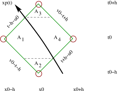
Figure 1: The cell that the particle crosses and the four areas defined to construct the second order algorithm.

2.1 Second order method

We next consider the integration of the potential term over the cell. If the cell is one not crossed by the particle, then we can use a trapezoidal rule

$$\int\int dA\left\{-V\psi\right\}=-h^{2}\left[V(r^{*})\psi(t+h,r^{*})+V(r^{*})\psi(t-h,r^{*})+\right.$$

$$\left.V(r^{*}+h)\psi(t,r^{*}+h)+V(r^{*}-h)\psi(t,r^{*}-h)\right]+{\cal O}(h^{4})\ .$$ (21)

The $h^{4}$ order error in a generic cell is equivalent to an overall ${\cal O}(h^{2})$ error in $\psi$ after a finite time of evolution.

The result in Eq. (2.1) assumes that $\psi$ is smooth in the grid cell. It cannot be applied to those cells through which the particle worldline passes, since $\psi$ is discontinuous across the worldline. For such cells we first obtain the coordinates $(r^{*}_{1},t_{1})$ of the point where the particle enters the cell and $(r^{*}_{2},t_{2})$ where the particle leaves it (see Fig. 1 for one of the four entering/exiting possible cases). Next, we divide the total area of the cell, $(4h^{2})$, into four subareas defined as follows: $A_{2}$ is the part of the area of the diamond below $t=t_{1}$, $A_{3}$ is the part of the area of the diamond over $t=t_{2}$, $A_{1}$ is the remaining area to the left of the particle’s trajectory, and $A_{4}$ is the remaining area to the right.

The integral of the $V\psi$ term over the area of the cell is approximated by the sum of this function evaluated on the corners of the cell multiplied by the corresponding sub-area $A_{i}$. This gives us

$$\int\int dA\left\{-V\psi\right\}= - V(r^{*})\left[\psi(t+h,r^{*})A_{3}+\psi(t,r^{*}+h)A_{4}\right.$$ (22)

$$+ \left.\psi(t,r^{*}-h)A_{1}+\psi(t-h,r^{*})A_{2}\right]+{\cal O}(h^{3}).$$

The truncation error in each such cell is of order $(h^{3})$, just enough to have quadratic convergence, since only one cell with the particle has to be evaluated per time step.

In summary, our numerical scheme, for cells through which the particle worldline does not pass, is to solve for $\psi(t+h,r^{*})$, using Eq. (2) and Eq. (2.1) representing the integral over a single cell of the homogeneous version of Eq. (1). For cells containing the worldline, Eq. (2), Eq. (22), and Eq. (20) are used instead. The evolution algorithm we use is then

$$\psi(t+h,r^{*})=-\psi(t-h,r^{*})+\left[\psi(t,r^{*}+h)+\psi(t,r^{*}-h)\right]\left[1-\frac{h^{2}}{2}V(r^{*})\right]+{\cal O}(h^{4})~{},$$ (23)

for cells not crossed by the particle, and

$$\psi(t+h,r^{*})= -\psi(t-h,r^{*})\left[1+\frac{V(r^{*})}{4}(A_{2}-A_{3})\right]$$ (24)

$$+\psi(t,r^{*}+h)\left[1-\frac{V(r^{*})}{4}(A_{4}+A_{3})\right]$$

$$+\psi(t,r^{*}-h)\left[1-\frac{V(r^{*})}{4}(A_{1}+A_{3})\right]$$

$$-\frac{1}{4}\left[1-\frac{V(r^{*})}{4}(A_{3})\right]\int\int{\cal S}dA+{\cal O}(h^{3})~{},$$

for the cells that the particle does cross [23, 27].

The above equations cannot, however, be used to initiate the evolution off the first hypersurface. If $t=0$ denotes the time at which we have the initial data in the form of $\psi(0,r^{*})$ and $\partial_{t}\psi(0,r^{*})$, we lack the values $\psi(t=-h)$, necessary to apply the evolution algorithm. We can, however, use a Taylor expansion to write

$$\psi(-h,r^{*})=\psi(+h,r^{*})-2h\partial_{t}\psi(0,r^{*})+{\cal O}(h^{3})\ .$$ (25)

The right hand side can be used in place of $\psi(-h,r^{*})$ in the the algorithm to evolve off the first hypersurface and algebraically solve for $\psi(+h,r^{*})$. It is important to note that this substitution is valid only if $\psi(t,r^{*})$ is not singular between $t=-h$ and $t=+h$. This requires that the particle worldline does not cross the vertical line at $r^{*}$ between $t=-h$ and $t=+h$. In setting up the computational grid, we have been careful always to avoid such a crossing.

For the special case when the source term does not contain derivatives of the Dirac’s Delta, i.e. $F\equiv 0$, the waveform is continuous, i.e. $C^{0}$. In this case we can still use the expression (2.1) for the integration over the potential term for all cells and obtain an overall error ${\cal O}(h^{3})$, thus producing a cubic convergent algorithm. This has a direct application for the integration of the Hilbert-Einstein field equations in the perturbative regime: In the harmonic gauge the general relativistic equations take the form of wave operators with source terms, given by the energy-stress-tensor, $T_{\mu\nu}$, proportional to Dirac’s deltas only (no derivatives of it) [Barack and Lousto in preparation.]

3 4th order Algorithm

As we have seen the only part of the integration algorithm that needs to be approximated on the numerical grid is that of the potential term $V(r^{*})\,\psi(t,r^{*})$. There are two cases to be considered separately: Those cells that the particle crosses and those that do not. For the later the integration is simpler and we will dealt with it first.

3.1 Vacuum case

For the sake of notational simplicity let us denote the integrand by

$$g(t,r^{*})\,\dot{=}\,V^{even,odd}_{\ell}(r^{*})\,\psi^{even,odd}_{\ell m}(t,r^{*}).$$ (26)

The integration over the cell of

$$\int\int_{Cell}g\,dA,$$ (27)

can be performed by a double Simpson [34] integral providing the required forth order accurate evolutions. In order to perform this integral with the Simpson method we need to evaluate $g$ at all the points shown in Fig. 2. The final result is

$$\int\int g\,dA=\left(\frac{h}{3}\right)^{2}\left\{g_{1}+g_{2}+g_{3}+g_{4}+4\left(g_{12}+g_{24}+g_{34}+g_{13}\right)+16g_{0}\right\}+{\cal O}\left(h^{6}\right).$$ (28)

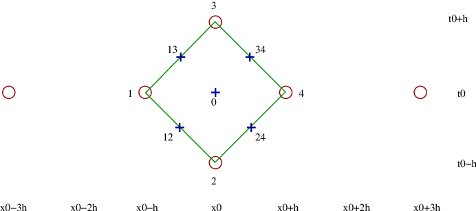
Figure 2: Vacuum case: the cells that the particle do no cross.

The use of this algorithm as it stands is possible but it implies to double the grid points in the time and space directions, and to retain information about four time slices, thus quadruplicating the number of points needed to evolve the same time interval.

It is possible though to evaluate the extra points (marked as crosses in Fig. 2) from the original grid points (marked as circles in Fig. 2). First, in order to avoid the central grid point, we can evaluate $g_{0}$ on the slice as follows

$$g_{0} = \frac{1}{16}\left[9V_{\ell}(x_{0}-h)\,\psi(t_{0},x_{0}-h)+9V_{\ell}(x_{0}+h)\,\psi(t_{0},x_{0}+h)\right.$$ (29)

$$\left.~{}~{}~{}-V_{\ell}(x_{0}-3h)\,\psi(t_{0},x_{0}-3h)-V_{\ell}(x_{0}+3h)\,\psi(t_{0},x_{0}+3h)\right]$$

$$~{}~{}~{}+{\cal O}\left(h^{4}\right)\quad\quad\quad\quad\quad\quad{\rm(centered)},$$

$$g_{0} = \frac{1}{16}\left[5V_{\ell}(x_{A})\,\psi(t_{0},x_{A})+15V_{\ell}(x_{A}+2h)\,\psi(t_{0},x_{A}+2h)\right.$$ (30)

$$\left.~{}~{}~{}-5V_{\ell}(x_{A}+4h)\,\psi(t_{0},x_{A}+4h)+V_{\ell}(x_{A}+6h)\,\psi(t_{0},x_{A}+6h)\right]$$

$$~{}~{}~{}+{\cal O}\left(h^{3}\right)\quad\quad\quad\quad\quad\quad(x_{A}:{\rm left~{}boundary)},$$

$$g_{0} = \frac{1}{16}\left[5V_{\ell}(x_{B})\,\psi(t_{0},x_{B})+15V_{\ell}(x_{B}-2h)\,\psi(t_{0},x_{B}-2h)\right.$$ (31)

$$\left.~{}~{}~{}-5V_{\ell}(x_{B}-4h)\,\psi(t_{0},x_{B}-4h)+V_{\ell}(x_{B}-6h)\,\psi(t_{0},x_{B}-6h)\right]$$

$$~{}~{}~{}+{\cal O}\left(h^{3}\right)\quad\quad\quad\quad\quad\quad(x_{B}:{\rm right~{}boundary)},$$

Since the boundary values are only used once per time step, ${\cal O}\left(h^{3}\right)$ is all we need to evaluate $g_{0}$.

In order to compute the points between the time levels of the original grid we use the second order evolution scheme, Eq. (23) adapted to the current case

$$g_{13}+g_{12} = V_{\ell}(x_{0}-h/2)\left(\psi_{13}+\psi_{12}\right)$$

$$= V_{\ell}(x_{0}-h/2)\left(\psi_{1}+\psi_{0}\right)\left[1-\frac{1}{2}\left(\frac{h}{2}\right)^{2}V_{\ell}(x_{0}-h/2)\right]+{\cal O}\left(h^{4}\right),$$

$$g_{24}+g_{34} = V_{\ell}(x_{0}+h/2)\left(\psi_{24}+\psi_{34}\right)$$

$$= V_{\ell}(x_{0}+h/2)\left(\psi_{0}+\psi_{4}\right)\left[1-\frac{1}{2}\left(\frac{h}{2}\right)^{2}V_{\ell}(x_{0}+h/2)\right]+{\cal O}\left(h^{4}\right).$$

This completes the computation for the cells not crossed by the particle. Note that including two more points (the circles labeled as $x_{0}\pm 3h$ in Fig. 2)) in the algorithm allowed us to avoid the evaluation of the field in five new points (the crosses in Fig. 2)).

3.2 Cells with the particle

The key idea here is to expand the function $g(t,x=r^{*})\,\dot{=}\,V(r^{*})\,\psi(t,r^{*})$ around the left/right vertexes of the cell labeled with 1 and 4 in Fig. 2 and integrate the left and right parts of the cell as defined by the trajectory of the particle. We next write down explicitly the four possible integrals to the left and the four to the right depending on the trajectory of the particle (entering/exiting the cell). Here we will assume the function $g(t,x)$ can be expanded as individual Taylor series on both sides of the of the trajectory of the particle. So, to the required order (since we only use this algorithm once per time step) we can write

$$g_{R,L}(t,x) = g[t_{0},x_{0}\pm h]+\frac{\partial g}{\partial x}[t_{0},x_{0}\pm h]\,\,(x-x_{0}\mp h)+$$ (34)

$$\frac{\partial g}{\partial t}[t_{0},x_{0}\pm h]\,\,(t-t_{0})+\frac{\partial^{2}g}{\partial x^{2}}[t_{0},x_{0}\pm h]\,\,\frac{(x-x_{0}\mp h)^{2}}{2}+$$

$$\frac{\partial^{2}g}{\partial t\partial x}[t_{0},x_{0}\pm h]\,\,(t-t_{0})\,(x-x_{0}\mp h)+$$

$$\frac{\partial^{2}g}{\partial t^{2}}[t_{0},x_{0}\pm h]\,\,\frac{(t-t_{0})^{2}}{2}+{\cal O}\left(h^{3}\right).$$

We give the explicit construction of the derivatives of the function $g(t,x)$ out of the evaluations of $g(t,x)$ at nearby grid points in the B.

3.2.1 Left side integral

:

i) This case is displayed in Fig. 3 and the integral over the potential term (in the shaded area) reads

$$\int_{t_{1}}^{t_{2}}\int_{x_{0}-h}^{x_{p}(t)}\,g_{L}(t,x)\,dt\,dx$$

$$=\int_{t_{1}}^{t_{0}}\,dt\int_{v_{0}-t-h}^{x_{p}(t)}\,g_{L}(t,x)\,dx+\int_{t_{0}}^{t_{2}}\,dt\int_{t-h-u_{0}}^{x_{p}(t)}\,g_{L}(t,x)\,dx.$$ (35)

Here $t_{1}$ and $t_{2}$ are respectively the times the particle enter and leaves the cell. Its radial trajectory given by $x_{p}(t)$. Note that the central point of the diamond $(u_{0}=t_{0}-x_{0},v_{0}=t_{0}+x_{0})$ is not a grid point.

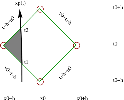
Figure 3: Case i), the particle enters (at time $t_{1}$) and leaves (at time $t_{2}$) the cell on the left side.

ii) This case is displayed in Fig. 4 and the integral over the potential (in the shaded area) term reads

$$\int_{t_{0}-h}^{t_{1}}\int_{x_{0}-h}^{x_{p}(t)}\,g_{L}(t,x)\,dt\,dx=\int_{t_{0}-h}^{t_{1}}\,dt\int_{v_{0}-t-h}^{t+h-u_{0}}\,g_{L}(t,x)\,dx$$

$$+\int_{t_{1}}^{t_{0}}\,dt\int_{v_{0}-t-h}^{x_{p}(t)}\,g_{L}(t,x)\,dx+\int_{t_{0}}^{t_{2}}\,dt\int_{t-h-u_{0}}^{x_{p}(t)}\,g_{L}(t,x)\,dx.$$ (36)

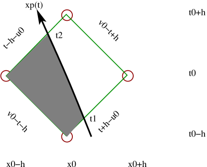
Figure 4: Case ii), the particle enters (at time $t_{1}$) on the right and leaves (at time $t_{2}$) the cell on the left side.

iii) This case is displayed in Fig. 5 and the integral over the potential term (in the shaded area) reads

$$\int_{t_{1}}^{t_{0}+h}\int_{x_{0}-h}^{x_{p}(t)}\,g_{L}(t,x)\,dt\,dx=\int_{t_{1}}^{t_{0}}\,dt\int_{v_{0}-t-h}^{x_{p}(t)}\,g_{L}(t,x)\,dx$$

$$+\int_{t_{0}}^{t_{2}}\,dt\int_{t-h-u_{0}}^{x_{p}(t)}\,g_{L}(t,x)\,dx+\int_{t_{2}}^{t_{0}+h}\,dt\int_{t-h-u_{0}}^{v_{0}-t+h}\,g_{L}(t,x)\,dx.$$ (37)

Figure 5: Case iii), the particle enters (at time $t_{1}$) on the left and leaves (at time $t_{2}$) the cell on the right side.

iv) This case is displayed in Fig. 6 and the integral over the potential term (in the shaded area) reads

$$\int_{t_{0}-h}^{t_{0}+h}\int_{x_{0}-h}^{x_{p}(t)}\,g_{L}(t,x)\,dt\,dx=\int_{t_{0}-h}^{t_{1}}\,dt\int_{v_{0}-t-h}^{t+h-u_{0}}\,g_{L}(t,x)\,dx$$

$$+\int_{t_{1}}^{t_{0}}\,dt\int_{v_{0}-t-h}^{x_{p}(t)}\,g_{L}(t,x)\,dx+\int_{t_{0}}^{t_{2}}\,dt\int_{t-h-u_{0}}^{x_{p}(t)}\,g_{L}(t,x)\,dx$$

$$+\int_{t_{2}}^{t_{0}+h}\,dt\int_{t-h-u_{0}}^{v_{0}-t+h}\,g_{L}(t,x)\,dx.$$ (38)

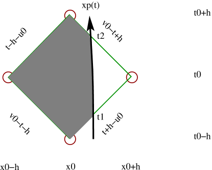
Figure 6: Case iv), the particle enters (at time $t_{1}$) and leaves (at time $t_{2}$) the cell on the right side.

3.2.2 Right side integral

:

i) This case is displayed in Fig. 3 and the integral over the potential term (in the non-shaded area) reads

$$\int_{t_{0}-h}^{t_{0}+h}\int^{x_{0}+h}_{x_{p}(t)}\,g_{R}(t,x)\,dt\,dx=\int_{t_{0}-h}^{t_{1}}\,dt\int_{v_{0}-t-h}^{t+h-u_{0}}\,g_{R}(t,x)\,dx$$

$$+\int_{t_{1}}^{t_{0}}\,dt\int^{t+h-u_{0}}_{x_{p}(t)}\,g_{R}(t,x)\,dx+\int_{t_{0}}^{t_{2}}\,dt\int^{v_{0}-t+h}_{x_{p}(t)}\,g_{R}(t,x)\,dx$$

$$+\int_{t_{2}}^{t_{0}+h}\,dt\int_{t-h-u_{0}}^{v_{0}-t+h}\,g_{R}(t,x)\,dx.$$ (39)

ii) This case is displayed in Fig. 4 and the integral over the potential term (in the non-shaded area) reads

$$\int_{t_{1}}^{t_{0}+h}\int^{x_{0}+h}_{x_{p}(t)}\,g_{R}(t,x)\,dt\,dx=\int_{t_{1}}^{t_{0}}\,dt\int^{t+h-u_{0}}_{x_{p}(t)}\,g_{R}(t,x)\,dx$$

$$+\int_{t_{0}}^{t_{2}}\,dt\int^{v_{0}-t+h}_{x_{p}(t)}\,g_{R}(t,x)\,dx+\int_{t_{2}}^{t_{0}+h}\,dt\int_{t-h-u_{0}}^{v_{0}-t+h}\,g_{R}(t,x)\,dx.$$ (40)

iii) This case is displayed in Fig. 5 and the integral over the potential term (in the non-shaded area) reads

$$\int_{t_{0}-h}^{t_{1}}\int^{x_{0}+h}_{x_{p}(t)}\,g_{R}(t,x)\,dt\,dx=\int_{t_{0}-h}^{t_{1}}\,dt\int_{v_{0}-t-h}^{t+h-u_{0}}\,g_{R}(t,x)\,dx$$

$$+\int_{t_{1}}^{t_{0}}\,dt\int^{t+h-u_{0}}_{x_{p}(t)}\,g_{R}(t,x)\,dx+\int_{t_{0}}^{t_{2}}\,dt\int^{v_{0}-t+h}_{x_{p}(t)}\,g_{R}(t,x)\,dx.$$ (41)

iv) This case is displayed in Fig. 6 and the integral over the potential term (in the non-shaded area) reads

$$\int_{t_{1}}^{t_{2}}\int^{x_{0}+h}_{x_{p}(t)}\,g_{R}(t,x)\,dt\,dx$$

$$=\int_{t_{1}}^{t_{0}}\,dt\int^{t+h-u_{0}}_{x_{p}(t)}\,g_{R}(t,x)\,dx+\int_{t_{0}}^{t_{2}}\,dt\int^{v_{0}-t+h}_{x_{p}(t)}\,g_{R}(t,x)\,dx.$$ (42)

For all these cases we can perform explicitly the first of the two integrals, then we need the explicit form of the trajectory to proceed further. We leave this for the direct numerical implementation since explicit expressions are straightforward but cumbersome.

4 Implementation

Here we will present the explicit implementation of the fourth order accurate algorithm in vacuum, the initial data and boundary conditions are also reviewed.

4.1 Initial data

While in the continuous Cauchy problem initial data of the second order partial differential equation (1) are specified by $\psi(t=0,x)$ and $\partial_{t}\psi(t=0,x)$, a numerical code needs data in previous time slices; in our case two. Assuming the field evolution can be expanded in a Taylor series in time around $t=0$

$$\psi(t,x)=\psi(0,x)+\partial_{t}\psi(0,x)\,\left(\frac{t}{1!}\right)+\partial_{t}^{2}\psi(0,x)\,\left(\frac{t^{2}}{2!}\right)+\partial_{t}^{3}\psi(0,x)\,\left(\frac{t^{3}}{3!}\right)+\partial_{t}^{4}\psi(0,x)\,\left(\frac{t^{4}}{4!}\right)+...,$$ (43)

where second and higher order time derivatives can be computed using the wave equation (1), i.e.,

$$\partial_{t}^{2}\psi(0,x)=\partial_{x}^{2}\psi(0,x)-V_{\ell}(x)\,\psi(0,x)+S_{\ell\,m}(0,x),$$ (44)

we can then obtain $\psi(h,x)$ to fourth order accurate in the integration step $h$ thus providing the two time levels to start the evolution algorithm.

Note that as pointed out in Ref. [23], this expansion requires the particle not to cross the line joining grid points at $t=0$ and $t=2h$. One can always choose carefully the location of the (staggered-characteristic) grid points such that this never happens for particles traveling at speeds less than that of the light.

4.2 Boundary conditions

The boundaries of the radial coordinate $x\,\dot{=}\,r^{*}$, that span the space outside the black hole from the horizon to spacial infinity, are taken at a finite distance from the hole, $x_{B}$ and from the event horizon $x_{A}$. At those boundaries we impose radiative conditions as purely ingoing near the horizon and purely outgoing at the outer boundary. These are clearly approximately true conditions which improve as we push further the boundaries.

At the outer boundary we assume then the radiative fall off

$$\psi(u,x)\approx F_{a}(u)+\frac{F_{b}(u)}{x}+\frac{F_{c}(u)}{x^{2}}+...$$ (45)

Evaluation of the above equation in three successive points along the constant $u$ direction give us the field at the boundary as a function of the two previous levels

$$\psi(t+h,x_{B})=\psi(t,x_{B}-h)+$$ (46)

$$\left[\psi(t,x_{B}-h)-\psi(t-h,x_{B}-2h)\right]\left(1-\frac{2h}{x_{B}}\right)+{\cal O}\left(\frac{1}{x_{B}^{2}}\right)+{\cal O}\left(h^{2}\right).$$

For the inner boundary, near the event horizon $x_{A}$ we have instead

$$\psi(v,x)\approx G_{a}(v)+\frac{G_{b}(v)}{x}+\frac{G_{c}(v)}{x^{2}}+...,$$ (47)

which leads to

$$\psi(t+h,x_{A})=\psi(t,x_{A}+h)+$$ (48)

$$\left[\psi(t,x_{A}+h)-\psi(t-h,x_{A}+2h)\right]\left(1+\frac{2h}{x_{A}}\right)+{\cal O}\left(\frac{1}{x_{A}^{2}}\right)+{\cal O}\left(h^{2}\right).$$

As we see, the expansions near the boundaries not only depend on the finite difference order, but also on the radiative condition that only applies approximately. This is apparent in the power dependence on the location of the numerical boundary and implies that pushing the boundaries further away will reduce the amplitude of the (spurious) reflected waves, but never completely eliminate its effects. In order to do that, one should use the exact treatment of the boundaries given in Ref. [15, 16].

4.3 Evolution in Vacuum

Using Eqs. (28)-(3.1) we can make explicit how to update the field $\psi$ using information on the two previous slices

$$\psi( t+h,x)=-\psi(t-h,x)+\left[1+\frac{1}{4}\left(\frac{h}{3}\right)^{2}\,V_{\ell}(x)\right]^{-1}\Biggr{\{}\psi(t,x-h)+\psi(t,x+h)$$ (49)

$$-\frac{1}{4}\left(\frac{h}{3}\right)^{2}\Biggr{[}V_{\ell}(x-h)\,\psi(t,x-h)+V_{\ell}(x+h)\,\psi(t,x+h)+16\,V_{\ell}(x)\,\psi(t,x)$$

$$+4\,\Bigg{[}V_{\ell}(x-h/2)\left(1-\frac{1}{2}\left(\frac{h}{2}\right)^{2}\,V_{\ell}(x-h/2)\right)\left(\psi(t,x-h)+\psi(t,x)\right)$$

$$+V_{\ell}(x+h/2)\left(1-\frac{1}{2}\left(\frac{h}{2}\right)^{2}\,V_{\ell}(x+h/2)\right)\left(\psi(t,x+h)+\psi(t,x)\right)\Bigg{]}\Biggr{]}\Biggr{\}},$$

where $(t,x)$ are the coordinates of the center of each cell (not a grid point), and $g_{0}=V_{\ell}(x)\,\psi(t,x)$ is given explicitly in Eq. (29)-(31).

To illustrate the numerical realization of the fourth order convergent algorithm we implemented the above formulae in a numerical code to compute waveforms as seen by an observer far away from the black holes (in this example at $r^{*}=430M$.) The initial distortion of the Schwarzschild black hole is produced by a Gaussian, time-symmetric perturbation

$$\psi(t=0,r^{*}) = A\exp\left[-(r^{*}-r_{c})^{2}/\sigma^{2}\right],$$ (50)

$$\partial_{t}\psi(t=0,r^{*}) = 0,$$ (51)

where $A,r_{c}$ and $\sigma$ are parameters that we have taken here as $1.0,3.0,1.0$ respectively.

To check the convergence rate we computed waveforms at three different resolutions $h,\ 2h$, and $4h$. In the example shown in Figs. 7 and 8, we have taken $h=M/8$. We computed the convergence rate simply as

$$n=\log\left|\frac{\psi(4h)-\psi(2h)}{\psi(2h)-\psi(h)}\right|/\log(2)+\log\left|\epsilon^{(n)}(\xi)\right|/\log(2),$$ (52)

where $\epsilon^{(n)}(\xi)$ represents the unknown error function of order $\approx 1$.

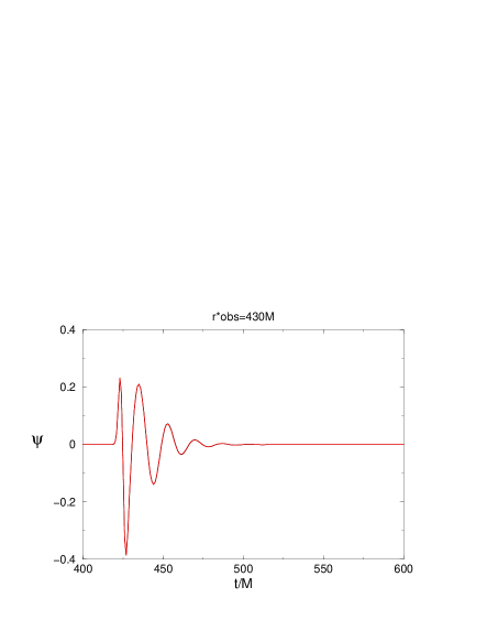
Figure 7: The Waveform of a Gaussian, time-symmetric initial pulse as seen by an observer located at $r^{*}=430M$. In this scale, second and fourth order evolution waveforms lie on top of each other.

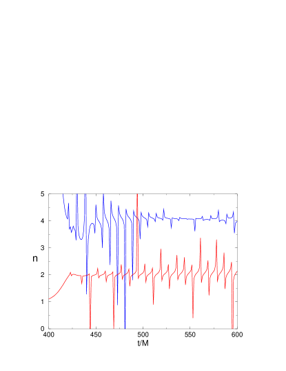
Figure 8: The converging power of the fourth versus the second order algorithms.

The plots show the desired fourth order convergence rate on average. For comparison we also implemented the second order algorithm (23) and displayed both rates together.

5 Discussion

Zerilli [39] has written down explicitly all ten field equations of General Relativity decomposed in tensor harmonics in the Regge-Wheeler gauge [35]. Then derived wave equations for both degrees of freedom of the gravitational field, i.e. even and odd parity perturbations, described in terms of (gauge invariant) waveforms build up of metric perturbations and its first derivatives. We described here how to integrate numerically in the time domain these wave equation, when the perturbations are due to an orbiting point-like source, represented by a Dirac’s delta. In order to complete the program we have to be able to reconstruct the metric perturbations. This was done in Refs. [19, 21], and applied to the radiation reaction problem in Refs. [19, 20, 7].

While we have a good understanding of perturbations due to an orbiting particle around nonrotating black holes, we still need to make the equivalent progress when dealing with perturbations of Kerr, i.e. rotating black holes. The Teukolsky equation [36] describes those (curvature) perturbations compactly as a wave equation for the Weyl scalars. It is straightforward to compute [9] the energy and momentum radiated to infinity by the system from the scalar $\Psi_{4}$. Yet, we need to reconstruct the metric perturbations to compute, for instance the force the particle exerts on itself and that accounts for the decay of orbits due to gravitational radiation (See Refs. [32, 33] for a review). Recently this problem has been tackled in the nonrotating limit [25, 21]. For the general Kerr background the problem remains open [see Ref. [30].]

In any case, the starting point is to numerically solve, the Teukolsky equation with an orbiting particle as a source. This plays very much the role of the Zerilli and Regge-Wheeler equations that we just have been dealing with. A first step has been recently taken by generalizing the second order [14] to fourth order [31] accurate formalism, yet in vacuum. The problem of generalizing the algorithms presented here for the orbiting particle to the Teukolsky equation remains as another open question in perturbation theory.

Appendix A Waveforms, Source terms and initial data

A.1 Even parity source terms

To obtain the Zerilli equation with sources for our waveform

$$\left[\partial_{r^{*}}^{2}-\partial_{t}^{2}-V_{\ell}^{even}(r)\right]\psi_{even}^{\ell m}(r,t)=S_{even}^{\ell m}(r,t),$$ (53)

we make the following combination of Einstein equations in the Regge-Wheeler gauge [See Eq. (2.13) of Ref. [22]]

$$\frac{2(1-2M/r)}{r(\lambda+1)(\lambda r+3M)}\left[r^{2}(1-2M/r)\partial_{r}R_{\theta\theta}\right.$$

$$\left.-(\lambda r+M)R_{\theta\theta}-\frac{\lambda r^{4}}{(\lambda r+3M)}G_{tt}+r^{3}R_{tt}\right],$$ (54)

and find the source term is given by

$$S_{even}^{\ell m} = 8\pi\,{\frac{\,\left(r-2\,M\right)^{2}\left(\lambda\,r-r+M\right)A_{\ell m}}{\left(\lambda+1\right)r\left(\lambda\,r+3\,M\right)}}+16\pi\,{\frac{\,\left(r-2\,M\right)^{2}B_{\ell m}}{\left(\lambda\,r+3\,M\right)\left(\lambda+1\right)^{1/2}}}$$ (55)

$$-8\pi\,{\frac{r\left({\lambda}^{2}{r}^{2}+8\,r\lambda\,M-{r}^{2}\lambda-9\,rM+27\,{M}^{2}\right)\,{A^{(0)}_{\ell m}}}{\left(\lambda+1\right)\left(\lambda\,r+3\,M\right)^{2}}}$$

$$+8\pi\,{\frac{\,\left(r-2\,M\right)^{2}\sqrt{2}\,G_{\ell m}}{\left(\lambda+1\right)\left(\lambda\,r+3\,M\right)}}-8\pi\,{\frac{\,\left(r-2\,M\right)\sqrt{2}\,F_{\ell m}}{\sqrt{\lambda\,\left(\lambda+1\right)}}}$$

$$-8\pi\,{\frac{\left(r-2\,M\right)^{3}\,\partial_{r}A_{\ell m}}{\left(\lambda+1\right)\left(\lambda\,r+3\,M\right)}}+8\pi\,{\frac{\left(r-2\,M\right){r}^{2}\,{\partial_{r}{A^{(0)}_{\ell m}}}}{\left(\lambda+1\right)\left(\lambda\,r+3\,M\right)}}.$$

Note that we had to reverse the sign of the (even) $t\,\theta$ component of the Einstein equations as given by Zerilli [39]. Thus the source term proportional to $B^{(0)}_{\ell m}$ changes sign.

The source term of the Zerilli equation (53) has now the following form

$$S_{even}^{\ell m}=F(t)\,\frac{\partial}{\partial_{r}}\delta[r-R(t)]+G(t)\,\delta[r-R(t)],$$ (56)

where

$$F_{even}(t)=-8\pi\,{\frac{{m_{0}}\,{U^{0}}\left(R-2\,M\right)\left(\left({\frac{d}{dt}}R\right)^{2}{R}^{2}-\left(R-2\,M\right)^{2}\right)}{\left(\lambda+1\right)\left(\lambda\,R+3\,M\right){R}^{2}}}\bar{Y}_{\ell m},$$

$$G_{even}(t)=16\,{\frac{\left({\frac{d}{dt}}R\right)\pi\,m_{0}\,U^{0}\left(R-2\,M\right){\frac{d}{dt}}\bar{Y}_{\ell m}}{\left(\lambda R+3\,M\right)\left(\lambda+1\right)}}$$

$$-8\,{\frac{\left(R-2\,M\right)U^{0}{m_{0}}\,\pi\,\bar{X}_{\ell m}\left({\frac{d}{dt}}\Theta\right){\frac{d}{dt}}\Phi}{\lambda\,\left(\lambda+1\right)}}$$

$$-4\,{\frac{\left(R-2\,M\right)U^{0}m_{0}\,\pi\,\left(\left({\frac{d}{dt}}\Theta\right)^{2}-\left(\sin(\theta)\right)^{2}\left({\frac{d}{dt}}\Phi\right)^{2}\right)\bar{W}^{\ell m}}{\lambda\,\left(\lambda+1\right)}}$$

$$+8\,{\frac{\bar{Y}_{\ell m}\pi\,m_{0}\,U^{0}\left(R-2\,M\right)^{2}\left(\left({\frac{d}{dt}}\Theta\right)^{2}+\left(\sin(\theta)\right)^{2}\left({\frac{d}{dt}}\Phi\right)^{2}\right)}{\left(\lambda R+3\,M\right)\left(\lambda+1\right)}}$$

$$+8\,{\frac{\bar{Y}_{\ell m}\pi\,m_{0}\,U^{0}\left({R}^{2}\lambda+6\,RM+6\,\lambda R\,M+3\,{M}^{2}+{R}^{2}{\lambda}^{2}\right)\left(\left({\frac{d}{dt}}R\right)\right)^{2}}{\left(\lambda R+3\,M\right)^{2}\left(\lambda+1\right)R}}$$

$$-8\,{\frac{\bar{Y}_{\ell m}\pi\,m_{0}\,U^{0}\left(R-2\,M\right)^{2}\left({R}^{2}\lambda+{R}^{2}{\lambda}^{2}+15\,{M}^{2}+6\,\lambda R\,M\right)}{{R}^{3}\left(\lambda+1\right)\left(\lambda R+3\,M\right)^{2}}},$$ (57)

and where $R,\Theta,\Phi$ give the trajectory of the orbiting particle in spherical coordinates and $W^{\ell m}$ is defined in Eq. (80).

A.2 Even Parity Initial data

In Refs. [23, 24] we have introduced a conformally flat index as a combination of metric perturbations

$$I_{\rm conf}^{even}\equiv H_{2}^{\ell m}-K^{\ell m}+\frac{2}{r}\left(1-\frac{3M}{r}\right)\ \left(h_{1}^{\ell m}-\frac{r^{2}}{2}\partial_{r}G^{\ell m}\right)-2\left(1-\frac{2M}{r}\right)\partial_{r}\left(h_{1}^{\ell m}-\frac{r^{2}}{2}\partial_{r}G^{\ell m}\right)\ .$$ (58)

which is gauge invariant, and clearly vanishes for a 3-geometry that is in conformally flat form, with $h_{1}^{\ell m}=0,G^{\ell m}=0$ and $H_{2}^{\ell m}=K^{\ell m}$. The computation of this gauge invariant quantity from $\psi_{even}^{\ell m}(r)$ is most easily described in the Regge-Wheeler gauge, where $I_{\rm conf}^{even}$ reduces to $H_{2}^{\ell m}-K^{\ell m}$.

Now making use of this $I_{\rm conf}^{even}$ in the Regge-Wheeler gauge and the expressions [21] for $H_{2}^{\ell m}$ and $K^{\ell m}$ in terms of the waveform $\psi_{even}^{\ell m}$ we can write

$$I_{\rm conf}^{even}=(r-2M)\partial^{2}_{r}\psi_{even}^{\ell m}+\frac{[(\lambda-3)r+9M]M}{(\lambda r+3M)r}\partial_{r}\psi_{even}^{\ell m}$$

$$-\frac{[27M^{3}+24\lambda M^{2}r+3\lambda(3\lambda+1)Mr^{2}+2\lambda^{2}(\lambda+1)r^{3}]}{(\lambda r+3M)^{2}r^{2}}\psi_{even}^{\ell m}$$ (59)

$$+\frac{\kappa\ U^{0}(1-2M/r)[\lambda(\lambda+1)r^{2}-3M^{2}]}{(\lambda+1)(\lambda r+3M)^{2}}\delta[r-R]-\frac{\kappa\ U^{0}(r-2M)^{2}}{(\lambda+1)(\lambda r+3M)}\partial_{r}\delta[r-R],$$

where $\kappa=8\pi m_{0}Y_{\ell m}[\Theta(t),\Phi(t)]$. This equation is completely equivalent to the Hamiltonian constraint [21]. It is only written in terms of the two variables $I_{\rm conf}^{even}$ and $\psi_{even}^{\ell m}$ instead of $H_{2}^{\ell m}$ and $K^{\ell m}$. The conformally flat initial data that we studied in Refs. [24] corresponds to choose $I_{\rm conf}^{even}=0$ and solve (with specified boundary conditions) for the resulting differential equation for $\psi_{even}^{\ell m}$.

Interestingly enough, the time derivative (represented by an overdot) of this equation

$$\dot{I}_{\rm conf}^{even} = (r-2M)\partial_{r}^{2}\dot{\psi}_{even}^{\ell m}+\frac{[(\lambda-3)r+9M]M}{(\lambda r+3M)r}\partial_{r}\dot{\psi}_{even}^{\ell m}$$ (60)

$$-\frac{[27M^{3}+24\lambda M^{2}r+3\lambda(3\lambda+1)Mr^{2}+2\lambda^{2}(\lambda+1)r^{3}]}{(\lambda r+3M)^{2}r^{2}}\dot{\psi}_{even}^{\ell m}$$

$$+\frac{2\kappa\ U^{0}\dot{R}[9M^{2}+2M(\lambda-3)r-\lambda(\lambda+3)r^{2}]}{(\lambda+1)r^{2}(\lambda r+3M)^{2}}\delta[r-R]$$

$$+\frac{8\pi m_{0}(d\bar{Y}_{\ell m}/dt)U^{0}(r-2M)(\lambda(\lambda+1)r^{2}-3M^{2})}{(\lambda+1)r(\lambda r+3M)^{2}}\delta[r-R]$$

$$+\frac{\kappa\,U^{0}\dot{r}_{p}(r-2M)[9M^{2}+2M\lambda r-\lambda(\lambda+1)r^{2}]}{(\lambda+1)r(\lambda r+3M)^{2}}\partial_{r}\delta[r-R]$$

$$-\frac{8\pi m_{0}(d\bar{Y}_{\ell m}/dt)U^{0}(r-2M)^{2}}{(\lambda+1)(\lambda r+3M)}\partial_{r}\delta[r-R]$$

$$+\frac{\kappa\ U^{0}\dot{R}(r-2M)^{2}}{(\lambda+1)(\lambda r+3M)}\partial_{r}^{2}\delta[r-R]\ .$$

is equivalent to the equations for the momentum constraint, i.e. when we replace the metric perturbations $K^{\ell m},H_{2}^{\ell m},H_{1}^{\ell m}$ into either the $(tr)$ or $(t\varphi)$ components of the General Relativity constraints [21], both yield Eq. (60) above.

By specifying conditions on $I_{\rm conf}$ and $\dot{I}_{\rm conf}$ on an initial hypersurface $\Sigma$ one can determine $\psi^{\ell m}_{t_{\Sigma}}$ and $\dot{\psi}^{\ell m}_{t_{\Sigma}}$ which is the initial data we need to evolve Zerilli’s equation. In Ref. [24] we have taken

$${I}_{\rm conf}|_{t_{\Sigma}}=0,~{}~{}\dot{I}_{\rm conf}|_{t_{\Sigma}}=0\ .$$ (61)

to determine the “convective initial data

$$\psi^{\ell m}_{even}|_{t_{\Sigma}}=\psi^{\ell m}_{even}(x^{k};x^{k}_{p}[t_{\Sigma}])$$ (62)

$$\dot{\psi}^{\ell m}_{even}|_{t_{\Sigma}}=\left.\frac{\partial\psi^{\ell m}_{even}(x^{k};x^{k}_{p}[t])}{\partial t}\right|_{t_{\Sigma}}=\left[\frac{dx^{j}_{p}[t]}{dt}\ \frac{\partial\psi^{\ell m}_{even}(x^{k};x^{k}_{p}[t])}{\partial x^{j}_{p}}\right]_{t_{\Sigma}}\ .$$ (63)

For the case of circular orbits this data takes the form

$$\psi^{\ell m}_{even}|_{t_{\Sigma}}=\frac{2m(R)}{\lambda+1}\frac{\sqrt{4\pi/(2\ell+1)}}{\lambda r+3M}r\sqrt{r/\bar{r}}$$ (64)

$$\times\begin{cases}\left(\lambda+1+M/r+\sqrt{1-2M/r}\left(\ell+\sqrt{\bar{r}/r}\right)\right)(\bar{R}/\bar{r})^{\ell}\quad&;\bar{r}>\bar{R},\\ \\ \left(\lambda+1+M/r+\sqrt{1-2M/r}\left(\sqrt{\bar{r}/r}-\ell-1\right)\right)(\bar{r}/\bar{R})^{\ell+1}\quad&;\bar{r}<\bar{R},\end{cases}$$

where $\bar{r}=1/4(\sqrt{r}+\sqrt{r-2M})^{2}$ is the isotropic coordinate.

$$\dot{\psi}^{\ell m}_{even}|_{t_{\Sigma}}=\left.-\left(\frac{d\Phi}{dt}\right)\frac{\partial\psi^{\ell m}_{even}}{\partial\Phi}\right|_{t_{\Sigma}}\ ,=\left.-im\Omega\,\psi^{\ell m}_{even}\right|_{t_{\Sigma}}\ ,$$ (65)

A.3 Odd parity source term

The Hilbert-Einstein equations in the Regge-Wheeler gauge for the odd parity sector (See Zerilli’s[39] equations (C6a)-(C6c)) [Note the corrections to the source terms]

$$\frac{\partial^{2}h_{0}^{\ell m}}{\partial r^{2}}-\frac{\partial^{2}h_{1}^{\ell m}}{\partial r\partial t}-\frac{2}{r}\frac{\partial h_{1}^{\ell m}}{\partial t}+\left[\frac{4M}{r^{2}}-\frac{2(\lambda+1)}{r}\right]\frac{h_{0}^{\ell m}}{r-2M}$$

$$= -\frac{8\pi\,rQ^{(0)}_{\ell m}}{(1-2M/r)\sqrt{(\lambda+1)}},$$

$$\frac{\partial^{2}h_{1}^{\ell m}}{\partial t^{2}}-\frac{\partial^{2}h_{0}^{\ell m}}{\partial r\partial t}+\frac{2}{r}\frac{\partial h_{0}^{\ell m}}{\partial t}+2\lambda(r-2M)\frac{h_{1}^{\ell m}}{r^{3}}$$

$$= \frac{8\pi\,i(r-2M)Q_{\ell m}}{\sqrt{(\lambda+1)}},$$

$$(1-2M/r)\frac{\partial h_{1}^{\ell m}}{\partial r}-\frac{1}{(1-2M/r)}\frac{\partial h_{0}^{\ell m}}{\partial t}+\frac{2M}{r^{2}}h_{1}$$

$$= -\frac{4\pi\,ir^{2}D_{\ell m}}{\sqrt{\lambda(\lambda+1)}},$$ (68)

where $Q^{(0)}_{\ell m},Q_{\ell m}$ and $D_{\ell m}$ give the multipole decomposition of the energy-momentum tensor.

One can use the above equations to write the metric perturbation in the Regge–Wheeler gauge

$$h_{0}^{\ell m}(r,t) = \frac{1}{2}(1-2M/r)\partial_{r}\left(r\psi^{\ell m}\right)+\frac{4\pi r^{3}Q^{(0)}_{\ell m}}{\lambda\sqrt{(\lambda+1)}},$$ (69)

$$h_{1}^{\ell m}(r,t) = \frac{1}{2}\frac{r}{(1-2M/r)}\partial_{t}\psi^{\ell m}+\frac{4\pi ir^{3}Q_{\ell m}}{\lambda\sqrt{(\lambda+1)}},$$ (70)

Taking the time derivative of Eq. (A.3) and the radial derivative of Eq. (A.3) allow us to reconstruct the Regge-Wheeler equation for odd parity perturbations

$$\left[\partial_{r^{*}}^{2}-\partial_{t}^{2}-V_{\ell}^{odd}(r)\right]\psi^{\ell m}(r,t)=S_{odd}^{\ell m}(r,t),$$ (71)

where the source is given by

$$S_{odd}^{\ell m}=-{\frac{8\pi\,\left(r-2\,M\right)}{\lambda\sqrt{\left(\lambda+1\right)}}}\left[{\frac{\partial}{\partial r}}\left(r{Q^{(0)}_{\ell m}}(r,t)\right)-ir{\frac{\partial}{\partial t}}Q(r,t)_{\ell m}\right].$$ (72)

For the Zerilli’s variable $\psi^{\ell m}_{Zer,odd}$ the source term looks like instead

$$S_{Zer,odd}^{\ell m} = \frac{8\pi\,i(1-2M/r)}{\sqrt{\lambda+1}}\left[-(1-2M/r)\,Q_{\ell m}+\frac{r}{\sqrt{2\lambda}}\partial_{r}\left((1-2M/r)D_{\ell m}\right)\right].$$

For a source term represented by a particle

$$Q^{(0)}_{\ell m} = \frac{m_{0}\,U^{0}(t)(1-2M/r)\,{\rm ang}(t)\,\delta[r-R(t)]}{r\sqrt{\lambda+1}},$$ (74)

$$Q_{\ell m} = \frac{i\,m_{0}\,U^{0}(t)(\frac{d}{dt}R)\,{\rm ang}(t)\,\delta[r-R(t)]}{(r-2M)\sqrt{\lambda+1}},$$ (75)

$$D_{\ell m} = -\frac{i\,m_{0}\,U^{0}(t)\,{\rm ang2}(t)\,\delta[r-R(t)]}{\sqrt{2\lambda(\lambda+1)}},$$ (76)

where

$${\rm ang}(t)=\frac{1}{\sin\Theta}\left(\frac{d\Theta}{dt}\right)\partial_{\varphi}\bar{Y}^{\ell m}(\Theta,\Phi)-\sin\Theta\left(\frac{d\Phi}{dt}\right)\partial_{\theta}\bar{Y}^{\ell m}(\Theta,\Phi),$$ (77)

$${\rm ang2}(t) = \frac{1}{2}\left[\left(\frac{d\Theta}{dt}\right)^{2}-\sin^{2}\Theta\left(\frac{d\Phi}{dt}\right)^{2}\right]$$ (78)

$$\times \left[\frac{1}{\sin\Theta}\bar{X}^{\ell m}\right]-\sin\Theta\frac{d\Phi}{dt}\frac{d\Theta}{dt}\bar{W}^{\ell m},$$

and $R,\Theta,\Phi$ define the trajectory of the orbiting particle in spherical coordinates. We also used Zerilli’s notation

$${X}^{\ell m} = 2\partial_{\varphi}\Big{(}\partial_{\theta}-\cot\theta\Big{)}Y^{\ell m},$$ (79)

$${W}^{\ell m} = \left(\partial^{2}_{\theta}-\cot\theta\,\partial_{\theta}-\frac{1}{\sin^{2}\theta}\partial^{2}_{\varphi}\right)Y^{\ell m}.$$ (80)

The source term of the Regge-Wheeler equation (71) has now the following form

$$S_{odd}^{\ell m}=F(t)\,\frac{\partial}{\partial_{r}}\delta[r-R(t)]+G(t)\,\delta[r-R(t)],$$ (81)

where

$$F(t) = -{\frac{8\pi\,{m_{0}}\,{U^{0}}(t)\left[(R-2M)^{2}-R^{2}(\partial_{t}R)^{2}\right]}{\lambda(\lambda+1)\,R}}{\rm ang}(t),$$ (82)

$$G(t)= - {\frac{8\pi{m_{0}}\,{U^{0}}(t)R\left({\frac{d}{dt}}R\right)\left({\frac{d}{dt}}{\rm ang}(t)\right)}{\lambda(\lambda+1)}}-{\frac{8\pi{m_{0}}\,{\rm ang}(t)}{\lambda(\lambda+1)R}}$$ (83)

$$\times \Bigg{\{}R^{2}\left({\frac{d}{dt}}{U^{0}}(t)\right){\frac{d}{dt}}R+R^{2}{U^{0}}(t){\frac{d^{2}}{d{t}^{2}}}R$$

$$+ 2M\,{U^{0}}(t)-R\,{U^{0}}(t)+R\,{U^{0}}(t)\left({\frac{d}{dt}}R\right)^{2}\Bigg{\}}.$$

A.4 Odd Parity Initial data

In analogy to the ’even’ conformally flat index we define the following combination of metric perturbations

$$I_{\rm conf}^{Odd}\equiv h_{1}^{\ell m}+\frac{r^{2}}{2}\partial_{r}\left(\frac{h_{2}^{\ell m}}{r^{2}}\right)\ .$$ (84)

which is gauge invariant, and clearly vanishes for a 3-geometry that is in conformally flat form. With $h_{2}^{\ell m}=0$ in the Regge-Wheeler gauge, an initially conformally flat metric $\left.I_{\rm conf}^{Odd}\right|_{\Sigma}=0$ means

$$\left.h_{1}^{\ell m}\right|_{\Sigma}=0.$$ (85)

Now taking also $\left.\dot{I}_{\rm conf}^{Odd}\right|_{t_{\Sigma}}=0$ in the Regge-Wheeler gauge leads to

$$\left.\partial_{t}h_{1}^{\ell m}\right|_{t_{\Sigma}}=0,$$ (86)

which is the Odd parity version of the CF thin-sandwich data with $\tilde{u}_{ij}=0$ (See Ref. [38, 10]). While $\dot{I}=0$ is the Wilson-Mathew  [26] approach adapted to black hole initial data. Other equivalent (at our perturbative level) formulation was given by [12, 13] proposing a helical Killing vector symmetry.

From Eq. (69) we see that (85) gives

$$I_{\rm conf}^{Odd}=0=>\left.\partial_{t}\psi^{\ell m}_{Odd}\right|_{t_{\Sigma}}=0,$$ (87)

and from the definition of the waveform (11) the condition $\dot{h}_{1}^{\ell m}=0$ gives

$$\partial_{t}I_{\rm conf}^{Odd}=0=>\left.\psi^{\ell m}_{Odd}\right|_{t_{\Sigma}}=\frac{r^{3}}{\lambda}\partial_{r}\left(\frac{h_{0}^{\ell m}}{r^{2}}\right).$$ (88)

The momentum constraint (A.3) then gives us the form of $h_{0}|_{t_{\Sigma}}$

$$\frac{\partial^{2}h_{0}}{\partial\xi^{2}}+\left[\frac{2}{\xi^{2}}-\frac{\ell(\ell+1)}{\xi}\right]\frac{h_{0}}{\xi-1}=-\frac{8\pi\,m_{0}\,U^{0}(t_{\Sigma})2M\,ang(t_{\Sigma})}{(\lambda+1)}\delta(\xi-\xi_{p}),$$

(89)

where $\xi=r/(2M)$ and $\xi_{p}=R(t)/(2M)$.

The solutions to this equation can be written in terms of hypergeometric functions

$$h_{0}^{\ell m}|_{t_{\Sigma}}=\begin{cases}{\rm C_{1}(\xi_{p})}y_{1}(\xi)~{},~{}~{}\xi\leq\xi_{p},\\ {\rm C_{2}(\xi_{p})}y_{2}(\xi)~{},~{}~{}\xi\geq\xi_{p},\\ \end{cases}$$ (90)

[Here we have the freedom of adding $y_{2}$ for all $\xi$ as an homogeneous solution representing additional ’radiation content’]. where

$$y_{1}(1) = {\xi}^{2}\left(\xi-1\right)^{-1+\ell}\,_{1}F_{2}\left([1-\ell,2-\ell],[-2\,\ell],-\left(\xi-1\right)^{-1}\right),$$ (91)

$$y_{2}(\xi) = {\xi}^{2}\left(\xi-1\right)^{-2-\ell}\,_{1}F_{2}\left([\ell+3,\ell+2],[2+2\,\ell],-\left(\xi-1\right)^{-1}\right).$$ (92)

In order to determine the value of the constant ${\rm C(\xi_{p})}$ we ensure the satisfaction of Eq. (89) at $r=R$ by equating the jump the the first derivatives of $h_{0}$ with the coefficient of the $\delta(\xi-\xi_{p})$ in the source term of Eq. (89). The result is

$$C_{1,2}(\xi_{p})=\left.8\pi\,m_{0}\,U^{0}(R)\,{\rm ang}^{\ell m}\left[\Theta(t_{\Sigma}),\Phi(t_{\Sigma})\right]\frac{2M}{(\lambda+1)}\frac{y_{1,2}}{W}\right|_{(\xi_{p})}$$ (93)

with $W=y_{1}^{\prime}\,y_{2}-y_{2}^{\prime}\,y_{1}=2\ell+1$.

For instance, for $\ell=2$ we get

$$\left.\psi^{\ell=2,m}\right|_{t_{\Sigma}}=\begin{cases}{\rm C_{1}}\,\frac{\xi^{3}}{\lambda}~{},~{}~{}\xi\leq\xi_{p},\\ \\ {\rm C_{2}}\,\left[-\frac{20\xi^{3}}{\lambda}\ln\left|\frac{\xi}{\xi-1}\right|+\frac{5(12\xi^{3}+6\xi^{2}+4\xi+3)}{3\lambda\xi}\right]~{},~{}~{}\xi\geq\xi_{p}.\end{cases}$$ (94)

For $\ell=3$ we get

$$\left.\psi^{\ell=2,m}\right|_{t_{\Sigma}}=\begin{cases}{\rm C_{1}}\,\frac{\xi^{3}}{\lambda}(2\xi-5/3)~{},~{}~{}\xi\leq\xi_{p},\\ \\ {\rm C_{2}}\,\left[-\frac{210\xi^{3}(6\xi-5)}{\lambda}\ln\left|\frac{\xi}{\xi-1}\right|+\frac{7(360\xi^{4}-120\xi^{3}-30\xi^{2}-10\xi-3)}{2\lambda\xi}\right]~{},~{}~{}\xi\geq\xi_{p}.\end{cases}$$ (95)

Successive multipoles can be computed in the same way when needed.

Appendix B Numerical construction of up to second order derivatives

In Sec. 3.2 we have assumed that we can Taylor expand the function $g(t,x)=V(x)\,\psi(t,x)$ around the left and right corners of the cell (centered at $(t_{0},x_{0}))$ the particle crosses

$$g_{R,L}(t,x) = g[t_{0},x_{0}\pm h]+\frac{\partial g}{\partial x}[t_{0},x_{0}\pm h]\,(x-x_{0}\mp h)+$$ (96)

$$\frac{\partial g}{\partial t}[t_{0},x_{0}\pm h]\,(t-t_{0})+\frac{\partial^{2}g}{\partial x^{2}}[t_{0},x_{0}\pm h]\,\frac{(x-x_{0}\mp h)^{2}}{2!}+$$

$$\frac{\partial^{2}g}{\partial t\partial x}[t_{0},x_{0}\pm h]\,(t-t_{0})\,(x-x_{0}\mp h)+$$

$$\frac{\partial^{2}g}{\partial t^{2}}[t_{0},x_{0}\pm h]\,\frac{(t-t_{0})^{2}}{2!}+{\cal O}\left(h^{3}\right).$$

So, for numerical purposes, we need to construct the derivatives appearing here in terms of the function evaluated in nearby grid points. The technique we use is to evaluate the Taylor expansion above (96) in six nearby point to evaluate $g$ and all up to second derivatives of $g$ at the left/right corner of the cell the particle crosses through.

B.1

Case i), the particle enters and leaves the cell on the left side. The construction of the derivatives is made taking into account the points labeled with the crossed circle on the left side, $\oplus$, and with the Xed-circle on the right, $\otimes$ [See Fig. 9.] To the required order, the derivatives in terms of grid points evaluations read explicitly

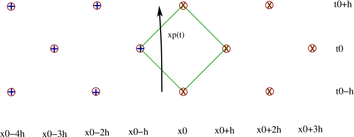
Figure 9: Case i) the particle enters and leaves to the left. The field $\psi$ is approximated by an expansion around the left corner of the cell using the points labeled by $\oplus$ and around the right corner by points labeled by $\otimes$.

For the integration on the left

$$\frac{\partial g_{L}}{\partial x}[t_{0},x_{0}-h]= \frac{4g(t_{0},x_{0}-h)+g(t_{0}+h,x_{0}-4h)+g(t_{0}-h,x_{0}-4h)}{4h}$$

$$-\frac{4g(t_{0},x_{0}-3h)+g(t_{0}-h,x_{0}-2h)+g(t_{0}+h,x_{0}-2h)}{4h},$$

$$\frac{\partial g_{L}}{\partial t}[t_{0},x_{0}-h]= \frac{3g(t_{0}+h,x_{0}-2h)-3g(t_{0}-h,x_{0}-2h)}{4h}$$ (98)

$$\frac{-g(t_{0}+h,x_{0}-4h)+g(t_{0}-h,x_{0}-4h)}{4h},$$

$$\frac{\partial^{2}g_{L}}{\partial x^{2}}[t_{0},x_{0}-h]= \frac{g(t_{0}+h,x_{0}-4h)+2g(t_{0},x_{0}-h)+g(t_{0}-h,x_{0}-4h)}{4h^{2}}$$

$$-\frac{g(t_{0}-h,x_{0}-2h)+g(t_{0}+h,x_{0}-2h)+2g(t_{0},x_{0}-3h)}{4h^{2}},$$

$$\frac{\partial^{2}g_{L}}{\partial t\partial x}[t_{0},x_{0}-h]= \frac{g(t_{0}-h,x_{0}-4h)-g(t_{0}-h,x_{0}-2h)}{4h^{2}}$$ (100)

$$\frac{-g(t_{0}+h,x_{0}-4h)+g(t_{0}+h,x_{0}-2h)}{4h^{2}},$$

$$\frac{\partial^{2}g_{L}}{\partial t^{2}}[t_{0},x_{0}-h]= \frac{3g(t_{0}-h,x_{0}-2h)-2g(t_{0},x_{0}-h)}{4h^{2}}$$

$$+\frac{g(t_{0}+h,x_{0}-4h)+g(t_{0}+h,x_{0}-2h)}{4h^{2}}$$

$$+\frac{g(t_{0}-h,x_{0}-4h)+3g(t_{0}+h,x_{0}-2h)-6g(t_{0},x_{0}-3h)}{4h^{2}},$$

and for the integration on the right

$$\frac{\partial g_{R}}{\partial x}[t_{0},x_{0}+h]= \frac{-g(t_{0}+h,x_{0}+2h)+g(t_{0}-h,x_{0})}{4h}$$ (102)

$$+\frac{g(t_{0}+h,x_{0})-g(t_{0}-h,x_{0}+2h)}{4h},$$

$$\frac{\partial g_{R}}{\partial t}[t_{0},x_{0}+h]= \frac{g(t_{0}+h,x_{0})-g(t_{0}-h,x_{0}+2h)}{4h}$$ (103)

$$\frac{-g(t_{0}-h,x_{0})+g(t_{0}+h,x_{0}+2h)}{4h},$$

$$\frac{\partial^{2}g_{R}}{\partial x^{2}}[t_{0},x_{0}+h]= \frac{-g(t_{0}+h,x_{0}+2h)-2g(t_{0},x_{0}+h)+g(t_{0}-h,x_{0})}{4h^{2}}$$

$$+\frac{g(t_{0}+h,x_{0})-g(t_{0}-h,x_{0}+2h)+2g(t_{0},x_{0}+3h)}{4h^{2}},$$

$$\frac{\partial^{2}g_{R}}{\partial t\partial x}[t_{0},x_{0}+h]= \frac{-g(t_{0}-h,x_{0})+g(t_{0}+h,x_{0})}{4h^{2}}$$ (105)

$$\frac{-g(t_{0}+h,x_{0}+2h)+g(t_{0}-h,x_{0}+2h)}{4h^{2}},$$

$$\frac{\partial^{2}g_{R}}{\partial t^{2}}[t_{0},x_{0}+h]= \frac{3g(t_{0}-h,x_{0}+2h)-6g(t_{0},x_{0}+h)-2g(t_{0},x_{0}+3h)}{4h^{2}}$$

$$+\frac{g(t_{0}-h,x_{0})+g(t_{0}+h,x_{0})+3g(t_{0}+h,x_{0}+2h)}{4h^{2}}.$$

B.2

Case ii), the particle enters the cell on the right side and leaves it on the left side. The construction of the derivatives is made taking into account the points labeled with the crossed circle on the left side, $\oplus$, and with the Xed-circle on the right, $\otimes$ [See Fig. 10.] Note that if we had chosen the alternative point $g(t_{0}+h,x_{0}-4h)$ instead of $g(t_{0}-h,x_{0}-4h)$ to the left, the set of equations do not produce a solution. The same applies to the right of the particle if we had taken $g(t_{0}-h,x_{0}+4h)$ instead of $g(t_{0}+h,x_{0}+4h)$ as the sixth grid point.

To the required order, the derivatives in terms of grid points evaluations read explicitly for the integration on the left

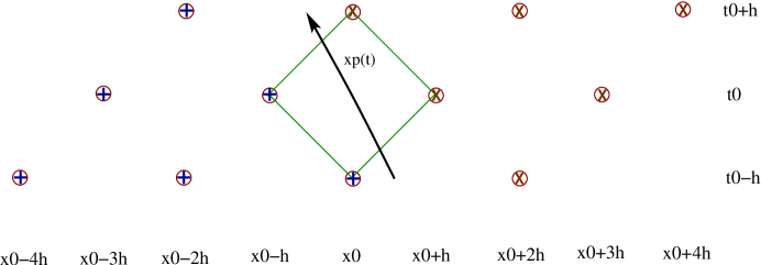
Figure 10: Case ii) the particle enters the cell on the right and leaves it on the left. The field $\psi$ is approximated by an expansion around the left corner of the cell using the points labeled by $\oplus$ and around the right corner by points labeled by $\otimes$.

$$\frac{\partial g_{L}}{\partial x}[t_{0},x_{0}-h]= \frac{-2g(t_{0},x_{0}-3h)+2g(t_{0},x_{0}-h)-2g(t_{0}-h,x_{0}-2h)}{4h}$$ (107)

$$+\frac{g(t_{0}-h,x_{0})+g(t_{0}-h,x_{0}-4h)}{4h},$$

$$\frac{\partial g_{L}}{\partial t}[t_{0},x_{0}-h]= \frac{-2g(t_{0}-h,x_{0}-2h)-g(t_{0}-h,x_{0})+2g(t_{0},x_{0}-h)}{4h}$$ (108)

$$\frac{-2g(t_{0},x_{0}-3h)+g(t_{0}-h,x_{0}-4h)+2g(t_{0}+h,x_{0}-2h)}{4h},$$

$$\frac{\partial^{2}g_{L}}{\partial x^{2}}[t_{0},x_{0}-h]= \frac{-2g(t_{0}-h,x_{0}-2h)+g(t_{0}-h,x_{0})+g(t_{0}-h,x_{0}-4h)}{4h^{2}},$$ (109)

$$\frac{\partial^{2}g_{L}}{\partial t\partial x}[t_{0},x_{0}-h]= \frac{-g(t_{0}-h,x_{0})+2g(t_{0},x_{0}-h)-2g(t_{0},x_{0}-3h)+g(t_{0}-h,x_{0}-4h)}{4h^{2}},$$

$$\frac{\partial^{2}g_{L}}{\partial t^{2}}[t_{0},x_{0}-h]= \frac{g(t_{0}-h,x_{0}-4h)-4g(t_{0},x_{0}-h)+g(t_{0}-h,x_{0})}{4h^{2}}$$ (111)

$$\frac{-4g(t_{0},x_{0}-3h)+4g(t_{0}+h,x_{0}-2h)+2g(t_{0}-h,x_{0}-2h)}{4h^{2}},$$

and for the integration on the right

$$\frac{\partial g_{R}}{\partial x}[t_{0},x_{0}+h]= \frac{-2g(t_{0},x_{0}+3h)+2g(t_{0},x_{0}+h)-2g(t_{0}+h,x_{0}+2h)}{4h}$$ (112)

$$+\frac{g(t_{0}+h,x_{0})+g(t_{0}+h,x_{0}+4h)}{4h},$$

$$\frac{\partial g_{R}}{\partial t}[t_{0},x_{0}+h]= \frac{g(t_{0}+h,x_{0})-2g(t_{0},x_{0}+h)-2g(t_{0}-h,x_{0}+2h)}{4h}$$ (113)

$$+\frac{2g(t_{0}+h,x_{0}+2h)-g(t_{0}+h,x_{0}+4h)+2g(t_{0},x_{0}+3h)}{4h},$$

$$\frac{\partial^{2}g_{R}}{\partial x^{2}}[t_{0},x_{0}+h]= \frac{-2g(t_{0}+h,x_{0}+2h)+g(t_{0}+h,x_{0})+g(t_{0}+h,x_{0}+4h)}{4h^{2}},$$ (114)

$$\frac{\partial^{2}g_{R}}{\partial t\partial x}[t_{0},x_{0}+h]= \frac{-g(t_{0}+h,x_{0}+4h)-2g(t_{0},x_{0}+h)+2g(t_{0},x_{0}+3h)+g(t_{0}+h,x_{0})}{4h^{2}},$$

$$\frac{\partial^{2}g_{R}}{\partial t^{2}}[t_{0},x_{0}+h]= \frac{4g(t_{0}-h,x_{0}+2h)-4g(t_{0},x_{0}+h)+2g(t_{0}+h,x_{0}+2h)}{4h^{2}}$$ (116)

$$+\frac{g(t_{0}+h,x_{0})+g(t_{0}+h,x_{0}+4h)-4g(t_{0},x_{0}+3h)}{4h^{2}}.$$

B.3

Case iii), the particle enters the cell on the left side and leaves it on the right side. The construction of the derivatives is made taking into account the points labeled with the crossed circle on the left side, $\oplus$, and with the Xed-circle on the right, $\otimes$ [See Fig. 11.] Note that if we had chosen the alternative point $g(t_{0}-h,x_{0}-4h)$ instead of $g(t_{0}+h,x_{0}-4h)$ to the left, the set of equations do not produce a solution. The same applies to the right of the particle if we had taken $g(t_{0}+h,x_{0}+4h)$ instead of $g(t_{0}-h,x_{0}+4h)$ as the sixth grid point.

To the required order, the derivatives in terms of grid points evaluations read explicitly for the integration on the left

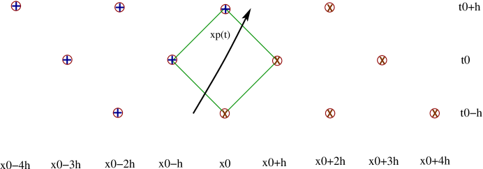
Figure 11: Case iii) the particle enters the cell on the left and leaves it on the right. The field $\psi$ is approximated by an expansion around the left corner of the cell using the points labeled by $\oplus$ and around the right corner by points labeled by $\otimes$ .

$$\frac{\partial g_{L}}{\partial x}[t_{0},x_{0}-h]= \frac{-2g(t_{0},x_{0}-3h)+2g(t_{0},x_{0}-h)-2g(t_{0}+h,x_{0}-2h)}{4h}$$ (117)

$$+\frac{g(t_{0}+h,x_{0})+g(t_{0}+h,x_{0}-4h)}{4h},$$

$$\frac{\partial g_{L}}{\partial t}[t_{0},x_{0}-h]= \frac{g(t_{0}+h,x_{0})-2g(t_{0},x_{0}-h)-2g(t_{0}-h,x_{0}-2h)}{4h}$$ (118)

$$+\frac{2g(t_{0}+h,x_{0}-2h)-g(t_{0}+h,x_{0}-4h)+2g(t_{0},x_{0}-3h)}{4h},$$

$$\frac{\partial^{2}g_{L}}{\partial x^{2}}[t_{0},x_{0}-h]= \frac{-2g(t_{0}+h,x_{0}-2h)+g(t_{0}+h,x_{0})+g(t_{0}+h,x_{0}-4h)}{4h^{2}},$$ (119)

$$\frac{\partial^{2}g_{L}}{\partial t\partial x}[t_{0},x_{0}-h]= \frac{-g(t_{0}+h,x_{0}-4h)-2g(t_{0},x_{0}-h)+2g(t_{0},x_{0}-3h)+g(t_{0}+h,x_{0})}{4h^{2}},$$

$$\frac{\partial^{2}g_{L}}{\partial t^{2}}[t_{0},x_{0}-h]= \frac{4g(t_{0}-h,x_{0}-2h)-4g(t_{0},x_{0}-h)+2g(t_{0}+h,x_{0}-2h)}{4h^{2}},$$ (121)

$$+\frac{g(t_{0}+h,x_{0})+g(t_{0}+h,x_{0}-4h)-4g(t_{0},x_{0}-3h)}{4h^{2}}$$

and for the integration on the right

$$\frac{\partial g_{R}}{\partial x}[t_{0},x_{0}+h]= \frac{-2g(t_{0},x_{0}+3h)+2g(t_{0},x_{0}+h)-2g(t_{0}-h,x_{0}+2h)}{4h}$$ (122)

$$+\frac{g(t_{0}-h,x_{0})+g(t_{0}-h,x_{0}+4h)}{4h},$$

$$\frac{\partial g_{R}}{\partial t}[t_{0},x_{0}+h]= \frac{-2g(t_{0}-h,x_{0}+2h)-g(t_{0}-h,x_{0})+2g(t_{0},x_{0}+h)-2g(t_{0},x_{0}+3h)}{4h}$$ (123)

$$+\frac{g(t_{0}-h,x_{0}+4h)+2g(t_{0}+h,x_{0}+2h)}{4h},$$

$$\frac{\partial^{2}g_{R}}{\partial x^{2}}[t_{0},x_{0}+h]= \frac{-2g(t_{0}-h,x_{0}+2h)+g(t_{0}-h,x_{0})+g(t_{0}-h,x_{0}+4h)}{4h^{2}},$$ (124)

$$\frac{\partial^{2}g_{R}}{\partial t\partial x}[t_{0},x_{0}+h]= \frac{-g(t_{0}-h,x_{0})+2g(t_{0},x_{0}+h)-2g(t_{0},x_{0}+3h)+g(t_{0}-h,x_{0}+4h)}{4h^{2}},$$

$$\frac{\partial^{2}g_{R}}{\partial t^{2}}[t_{0},x_{0}+h]= \frac{g(t_{0}-h,x_{0}+4h)-4g(t_{0},x_{0}+h)+g(t_{0}-h,x_{0})-4g(t_{0},x_{0}+3h)}{4h^{2}}$$ (126)

$$+\frac{4g(t_{0}+h,x_{0}+2h)+2g(t_{0}-h,x_{0}+2h)}{4h^{2}}.$$

B.4

Case iv), the particle enters and leaves the cell on the right side. The construction of the derivatives is made taking into account the points labeled with the crossed circle on the left side, $\oplus$, and with the Xed-circle on the right, $\otimes$ [See Fig. 12.] To the required order, the derivatives in terms of grid points evaluations read explicitly

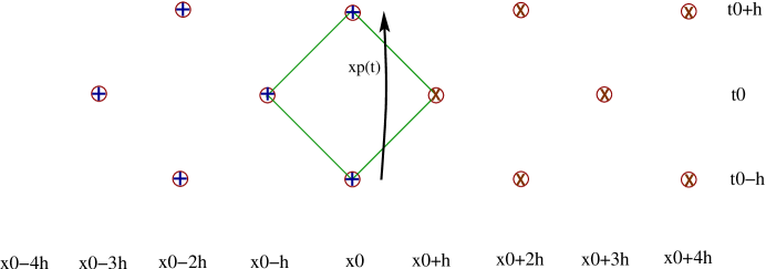
Figure 12: Case iv) the particle enters and leaves the cell on the right. The field $\psi$ is approximated by an expansion around the left corner of the cell using the points labeled by $\oplus$ and around the right corner by points labeled by $\otimes$.

For the integration on the left

$$\frac{\partial g_{L}}{\partial x}[t_{0},x_{0}-h]= \frac{-g(t_{0}+h,x_{0}-2h)+g(t_{0}-h,x_{0})+g(t_{0}+h,x_{0})-g(t_{0}-h,x_{0}-2h)}{4h},$$

$$\frac{\partial g_{L}}{\partial t}[t_{0},x_{0}-h]= \frac{g(t_{0}+h,x_{0})-g(t_{0}-h,x_{0}-2h)-g(t_{0}-h,x_{0})+g(t_{0}+h,x_{0}-2h)}{4h},$$

$$\frac{\partial^{2}g_{L}}{\partial x^{2}}[t_{0},x_{0}-h]= \frac{-g(t_{0}+h,x_{0}-2h)-2g(t_{0},x_{0}-h)+g(t_{0}-h,x_{0})}{4h^{2}}$$ (129)

$$+\frac{g(t_{0}+h,x_{0})-g(t_{0}-h,x_{0}-2h)+2g(t_{0},x_{0}-3h)}{4h^{2}},$$

$$\frac{\partial^{2}g_{L}}{\partial t\partial x}[t_{0},x_{0}-h]= \frac{-g(t_{0}-h,x_{0})+g(t_{0}+h,x_{0})-g(t_{0}+h,x_{0}-2h)+g(t_{0}-h,x_{0}-2h)}{4h^{2}},$$

$$\frac{\partial^{2}g_{L}}{\partial t^{2}}[t_{0},x_{0}-h]= \frac{3g(t_{0}-h,x_{0}-2h)-6g(t_{0},x_{0}-h)-2g(t_{0},x_{0}-3h)}{4h^{2}}$$ (131)

$$+\frac{g(t_{0}-h,x_{0})+g(t_{0}+h,x_{0})+3g(t_{0}+h,x_{0}-2h)}{4h^{2}},$$

and for the integration on the right

$$\frac{\partial g_{R}}{\partial x}[t_{0},x_{0}+h]= \frac{4g(t_{0},x_{0}+h)+g(t_{0}+h,x_{0}+4h)+g(t_{0}-h,x_{0}+4h)}{4h}$$

$$-\frac{4g(t_{0},x_{0}+3h)+g(t_{0}-h,x_{0}+2h)+g(t_{0}+h,x_{0}+2h)}{4h},$$

$$\frac{\partial g_{R}}{\partial t}[t_{0},x_{0}+h]= \frac{3g(t_{0}+h,x_{0}+2h)-3g(t_{0}-h,x_{0}+2h)}{4h}$$ (133)

$$\frac{-g(t_{0}+h,x_{0}+4h)+g(t_{0}-h,x_{0}+4h)}{4h},$$

$$\frac{\partial^{2}g_{R}}{\partial x^{2}}[t_{0},x_{0}+h]= \frac{g(t_{0}+h,x_{0}+4h)+2g(t_{0},x_{0}+h)+g(t_{0}-h,x_{0}+4h)}{4h^{2}}$$

$$-\frac{g(t_{0}-h,x_{0}+2h)+g(t_{0}+h,x_{0}+2h)+2g(t_{0},x_{0}+3h)}{4h^{2}},$$

$$\frac{\partial^{2}g_{R}}{\partial t\partial x}[t_{0},x_{0}+h]= \frac{g(t_{0}-h,x_{0}+4h)-g(t_{0}-h,x_{0}+2h)}{4h^{2}}$$ (135)

$$\frac{-g(t_{0}+h,x_{0}+4h)+g(t_{0}+h,x_{0}+2h)}{4h^{2}},$$

$$\frac{\partial^{2}g_{R}}{\partial t^{2}}[t_{0},x_{0}+h]= \frac{3g(t_{0}-h,x_{0}+2h)-2g(t_{0},x_{0}+h)}{4h^{2}}$$

$$\frac{+g(t_{0}+h,x_{0}+4h)+g(t_{0}+h,x_{0}+2h)}{4h^{2}}$$

$$\frac{+g(t_{0}-h,x_{0}+4h)+3g(t_{0}+h,x_{0}+2h)-6g(t_{0},x_{0}+3h)}{4h^{2}}.$$

References

References

- [1] J. Baker, S. R. Brandt, M. Campanelli, C. O. Lousto, E. Seidel, and R. Takahashi, Nonlinear and perturbative evolution of distorted black holes: Odd-parity modes, Phys. Rev. D 62 (2000), 127701, gr-qc/9911017.
- [2] J. Baker, B. Brügmann, Manuela Campanelli, C. O. Lousto, and R. Takahashi, Plunge waveforms from inspiralling binary black holes, Phys. Rev. Lett. 87 (2001), 121103.
- [3] J. Baker, M. Campanelli, C. O. Lousto, and R. Takahashi, Modeling gravitational radiation from coalescing binary black holes, Phys. Rev. D 65 (2002), 124012.
- [4] , Coalescence remnant of spinning binary black holes, Phys. Rev. D 69 (2004), 027505.
- [5] John Baker, Bernd Brügmann, Manuela Campanelli, and Carlos O. Lousto, Gravitational waves from black hole collisions via an eclectic approach, Class. Quantum Grav. 17 (2000), L149–L156.
- [6] John Baker, Manuela Campanelli, and Carlos O. Lousto, The Lazarus project: A pragmatic approach to binary black hole evolutions, Phys. Rev. D 65 (2002), 044001.
- [7] Leor Barack and Carlos O. Lousto, Computing the gravitational self-force on a compact object plunging into a schwarzschild black hole, Phys. Rev. D 66 (2002), 061502.
- [8] M. Campanelli and C. O. Lousto, The imposition of Cauchy data to the Teukolsky equation I: The nonrotating case, Phys. Rev. D 58 (1998), 024015.
- [9] M. Campanelli and C. O. Lousto, Second order gauge invariant gravitational perturbations of a Kerr black hole, Phys. Rev. D 59 (1999), 124022.
- [10] Gregory B. Cook, Corotating and irrotational binary black holes in quasi-circular orbits, Phys. Rev. D 65 (2002), 084003.
- [11] C. T. Cunningham, R. H. Price, and V. Moncrief, Radiation from collapsing relativistic stars. I. Linearized odd-parity radiation, Astrophys. J. 224 (1978), 643.
- [12] Eric Gourgoulhon, Philippe Grandclément, and Silvano Bonazzola, Binary black holes in circular orbits. I. A global spacetime approach, Phys. Rev. D 65 (2002), 044020.
- [13] Philippe Grandclément, Eric Gourgoulhon, and Silvano Bonazzola, Binary black holes in circular orbits. II. Numerical methods and first results, Phys. Rev. D 65 (2002), 044021.
- [14] W. Krivan, P. Laguna, Philippos Papadopoulos, and N. Andersson, Phys. Rev. D 56 (1997), 3395–3404.
- [15] S. R. Lau, Rapid evaluation of radiation boundary kernels for time- domain wave propagation on black holes: Implementation and numerical tests, Class. Quant. Grav. 21 (2004), 4147–4192.
- [16] Stephen R. Lau, Rapid evaluation of radiation boundary kernels for time- domain wave propagation on blackholes, J. Comput. Phys. 199 (2004), 376–422.
- [17] A. A. Logunov, M. A. Mestvirishvili, and V. A. Petrov, How were the hilbert-einstein equations discovered?, Phys. Usp. 47 (2004), 607–621.
- [18] C. O. Lousto and Richard H. Price, Radiation content of conformally flat initial data, Phys. Rev. D 69 (2004), 087503.
- [19] Carlos O. Lousto, Pragmatic Approach to Gravitational Radiation Reaction in Binary Black Holes, Phys. Rev. Lett. 84 (2000), 5251.
- [20] , Towards the solution of the relativistic gravitational radiation reaction problem for binary black holes, Class. Quantum Grav. 18 (2001), 3989.
- [21] Carlos O. Lousto, Reconstruction of black hole metric perturbations from weyl curvature ii: The regge-wheeler gauge, (2005).
- [22] Carlos O. Lousto and Richard H. Price, Headon collisions of black holes: The particle limit, Phys. Rev. D 55 (1997), 2124–2138.
- [23] , Understanding initial data for black hole collisions, Phys. Rev. D 56 (1997), 6439–6457.
- [24] , Improved initial data for black hole collisions, Phys. Rev. D 57 (1998), 1073–1083.
- [25] Carlos O. Lousto and Bernard F. Whiting, Reconstruction of black hole metric perturbations from weyl curvature, Phys. Rev. D 66 (2002), 024026.
- [26] P. Marronetti, G. J. Mathews, and J. R. Wilson, Irrotational binary neutron stars in quasi-equilibrium, Phys. Rev. D 60 (1999), 087301.
- [27] Karl Martel and Eric Poisson, A one-parameter family of time-symmetric initial data for the radial infall of a particle into a Schwarzschild black hole, Phys. Rev. D 66 (2002), 084001, gr-qc/0107104.
- [28] Mark Miller, Accuracy requirements for the calculation of gravitational waveforms from coalescing compact binaries in numerical relativity, (2005).
- [29] V. Moncrief, Gravitational perturbations of spherically symmetric systems. I. the exterior problem, Annals of Physics 88 (1974), 323–342.
- [30] Amos Ori, Reconstruction of inhomogeneous metric perturbations and electromagnetic four-potential in kerr spacetime, Phys. Rev. D 67 (2003), 124010.
- [31] Enrique Pazos-Ávalos and Carlos O. Lousto, Numerical integration of the teukolsky equation in the time domain, (2004).
- [32] E. Poisson, The Motion of Point Particles in Curved Spacetime, Living Reviews in Relativity 7 (2004), 6–+.
- [33] Eric Poisson, The gravitational self-force, (2004).
- [34] W. H. Press, B. P. Flannery, S. A. Teukolsky, and W. T. Vetterling, Numerical recipes, Cambridge University Press, Cambridge, England, 1986.
- [35] T. Regge and J. Wheeler, Stability of a Schwarzschild singularity, Phys. Rev. 108 (1957), no. 4, 1063–1069.
- [36] S. A. Teukolsky, Perturbations of a rotating black hole. I. fundamental equations for gravitational, electromagnetic, and neutrino-field perturbations, Astrophys. J. 185 (1973), 635–647.
- [37] Ivan T. Todorov, Einstein and hilbert: The creation of general relativity, (2005).
- [38] J. W. York, Conformal ‘thin-sandwich’ data for the initial-value problem of general relativity, Phys. Rev. Lett. 82 (1999), 1350–1353.
- [39] F. J. Zerilli, Gravitational field of a particle falling in a Schwarzschild geometry analyzed in tensor harmonics, Phys. Rev. D. 2 (1970), 2141.
- [40] Y. Zlochower, J. G. Baker, M. Campanelli, and C. O. Lousto, Accurate black hole evolutions by fourth-order numerical relativity, (2005).