Microwave Apparatus for Gravitational Waves Observation

Abstract

In this report the theoretical and experimental activities for the development of superconducting microwave cavities for the detection of gravitational waves are presented.

Introduction

Existing proposals for next–generation Earth–based gravitational wave detectors, including advanced interferometers (IFOs) and wideband (nested) acoustic detectors, are aimed at constructing large–scale prototypes, with strain sensitivity goals of the order of $10^{-23}$ in a wide (a few kHz) band. The successful achievement of these goals will depend on substantial advances to be made, well beyond the limits of presently achieved figures of merit, in several critical areas, including (ultra)cryogenics (mK cryostats with adequate refrigerating power), material science (achieving extremely high mechanical quality factors at cryogenic temperatures) and technology (annealing/sintherizing high–quality deca–ton size objects), electronics (SQL amplifiers), lasers and optics (high–finesse, large–waist, short optical cavities performing as displacement readouts at sensitivity levels $\sim 10^{-23}$ m Hz^-1/2). All these goals are two order of magnitude beyond the best figures available today, on average.

The MAGO proposal stems from a different perspective, and emphasizes a relatively new concept. The MAGO design aims at constructing a relatively large ($N\gtrsim 10$) number of detectors, relying only on available and already proven technology.

Experience gained on downsized MAGO prototypes suggests that MAGOs will be relatively cheap, compact–sized, and structurally simple. Indeed, within the limits of available and already proven technologies, the proposed MAGO design could allow to construct compact detectors, featuring strain sensitivities comparable to those of present day cryogenic acoustical detectors, at a fraction of their size and cost. This would permit to place several MAGOs even in a small area (which would be required, e.g., for observing a stochastic GW background), either co–tuned or frequency staggered, thanks to the unique bandwidth and center frequency tuning ease offered by the design.

The potential advantages of many–detector arrays and networks have been repeatedly emphasized. Similar to radioastronomy, gravitational wave astronomy will be eventually made possible by the availability of large assemblies of co–tuned (array) or frequency staggered (xylophone) detectors featuring robust, high duty–cycle operation, as a result of constructive simplicity, and non critical core technologies. The MAGO project and design is definitely aimed at moving a first, perhaps tiny step toward this direction.

The following specific technical points are worth being emphasized:

• The individual MAGO bandwidth and center frequency of operation can be easily tuned well beyond the operational limits of present day detectors, imposed by laser shot noise (IFOs) and Brownian (acoustic) noise;

• The very large parametric–conversion gain which provides the basic principle of operation of the detector brings the equivalent temperature of the front-end electronics down to the standard quantum limit already using standard, cheap and reliable off-the-shelf HEMT amplifier ($T\sim 2$ K at $1$ GHz), without the need of resorting to more sophisticated devices;

• The required electrical quality factor for the Nb-coated superconducting cavities, has been safely and routinely achieved in accelerator technology, and could be realistically improved by one order of magnitude relatively soon;

• The required mechanical quality factor of the cavities is also conservative and could be improved;

• The phase noise of the microwave pumping signal is well within the limits of currently available technology.

The main technology challenge is thus essentially related to the design and testing of a cryostat capable of removing the heat produced in the cavity walls by the microwave pumping signal (a few Watts, typically) so as to maintain an operating temperature $\sim 2$ K, while guaranteeing adequate acoustical isolation and very low intrinsic noise.

On the other hand, it should be noted that the MAGO design has no a–priori intrinsic limitation which could prevent it from reaching performance figures, both in terms of strain sensitivity and bandwidth, comparable to those of proposed next generation large–scale detectors (including advanced IFOs and wideband nested acoustic detectors), provided one pushes the relevant critical design figures (cryogenics, mass, mechanical quality factor, readout noise) up to comparable levels.

In particular, if we were able to design and operate the cryostat down to the mK range, the MAGO strain sensitivity could easily reach the $h\sim 10^{-23}$ level, while preserving MAGO’s almost unique features in terms of center frequency and bandwidth easy tunability. As of today, the best performing 100mK cryostats are capable of delivering only a few hundred mW. We note that next generation optically read–out wideband nested–acoustical detector would face the same technological challenge, among others, in order to reach their foreseen sensitivity goal.

I Experiment Overview

In the last decades, several laboratories all around the world have promoted an intense effort devoted to the direct detection of gravitational waves. The detectors, both those in operation and those being developed, belong to two conceptually different families, massive elastic solids (cylinders or spheres) websbarre and Michelson interferometers webinterf . Both types of detectors are based on the mechanical coupling between the gravitational wave and a test mass, and in both types the electromagnetic field is used as motion transducer.

In a series of papers, since 1978, it has been studied how the energy transfer induced by the gravitational wave between two levels of an electromagnetic resonator, whose frequencies $\omega_{1}$ and $\omega_{2}$ are both much larger than the characteristic angular frequency $\Omega$ of the g.w., could be used to detect gravitational waves bppr1 ; bppr2 . The energy transfer is maximum when the resonance condition $|\omega_{2}-\omega_{1}|=\Omega$ is satisfied. This is an example of a frequency converter, i.e. a nonlinear device in which energy is transferred from a reference frequency to a different frequency by an external pump signal.

In the scheme suggested by Bernard et al. the two levels are obtained by coupling two identical high frequency cavities bppr2 . Each resonant mode of the individual cavity is then split in two modes of the coupled resonator with different spatial field distribution. In the following we shall call them the symmetric and the antisymmetric mode. The frequency difference of the two modes (the detection frequency) is determined by the coupling, and can be tuned by a careful resonator design. An important feature of this device is that the detection frequency does not depend on its mechanical properties (dimensions, weight and mechanical modes resonant frequencies), though, of course, the detector can be tuned so that the mode splitting equals the frequency of a mechanical resonant mode. The sensitivity in this and other experimental situations will be discussed in the following. Since the detector sensitivity is proportional to the electromagnetic quality factor, ${\mathcal{Q}}$, of the resonator, superconducting cavities should be used for maximum sensitivity.

An R&D effort, started in 1998, was completed at the end of 2003 rsi ; cqg . Its main objective was the development of a tunable detector of small harmonic displacements based on two coupled superconducting cavities. Several cavity prototypes (both in copper and in niobium) were built and tested, and finally a design based on two spherical cells was chosen and realized (Fig. 1). The detection frequency, i.e. the frequency difference between the symmetric and antisymmetric modes, was chosen to be: $\omega_{2}-\omega_{1}\approx 10$ kHz (the frequency of the modes being $\omega_{1,2}\approx 2$ GHz). An electromagnetic quality factor ${\mathcal{Q}}>10^{10}$ was measured on a prototype with fixed coupling.

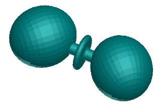
Figure 1: Artistic view of the coupled spherical cavities with the central tuning cell

The tuning system was also carefully studied. The coupling strength, and thus the tuning range, is determined by the diameter of the coupling tube and by the distance between the two sperical cells. A central elliptical cell, which can easily be streched and squeezed, was found to provide a tuning range of several kHz (4–20 kHz in the final design). A prototype with the central elliptical cell was built and tested (Fig. 2).

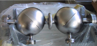
Figure 2: Niobium spherical cavities (variable coupling)

The system was also mechanically characterized, and the mechanical resonant modes in the frequency range of interest were identified. In particular the quadrupolar mode of the sphere was found to be at 4 kHz, in good agreement with finite elements calculations.

The detection electronics was designed. Its main task is to provide the rejection of the symmetric mode component at the detection frequency. A rejection better than 150 dB was obtained in the final system.

Starting from the results obtained in the last six years, we are now planning to design and realize an experiment for the detection of gravitational waves in the 4–10 kHz frequency range. Our main task is the design and construction of the refrigerator and of the cryostat (including the suspension system), which houses the coupled cavities. The refrigerator must provide the cryogenic power needed to keep the superconductiong cavities at $T\approx 1.8$ K (approx. 10 Watts) without introducing an excess noise from the external environment. A design based on the use of subcooled superfluid helium is being invesigated.

In the following a detailed description of the various issues aforementioned will be given. Expected system sensitivity will also be discussed.

II Physics Motivation

The spectrum of gravitational waves of cosmic origin targeted by currently operating or planned detectors spans roughly from $10^{-4}$ to $10^{4}$ Hz.

The $f\leq 10^{-1}$ Hz region of the GW spectrum, including galactic binaries gal_bin , (super)massive BH binary inspirals and mergers SMBH , compact object inspirals and captures by massive BHs capture , will be thoroughly explored by LISA LISA , which might be hopefully flown by year 2015. Ground based interferometers and acoustic detectors (bars and spheres) will likewise co–operate in exploring the $f\geq 10^{1}Hz$ region of the spectrum, including compact binary inspirals and mergers CB_inspiral , supernovae and newborn black-hole ringings SN_BHring , fast-spinning non-axisymmetric neutron stars NS , and stochastic GW background stochastic .

The whole spectral range from $10^{-4}-10^{4}$ Hz, however, is far from being covered with uniform sensitivity. Plans are being made for small–scale LISA–like space experiments (e.g., DECIGO, DECIGO ) aimed at covering the frequency gap $10^{-1}-10^{1}$ Hz between LISA and terrestrial detectors.

Several cryogenic/ultracryogenic acoustic (bar) detectors are also operational, including ALLEGRO ALLEGRO , AURIGA AURIGA , EXPLORER EXPLORER , NAUTILUS NAUTILUS , and NIOBE NIOBE . They are tuned at $\sim 10^{3}$ Hz, with bandwidths of a few tens of Hz, and minimal noise PSDs of the order of $10^{-21}$ Hz^-1/2.

Intrinsic factors exist which limit the performance of both IFOs and acoustic detectors in the upper frequency decade ($f\gtrsim 10^{3}$ Hz) of the spectrum.

The high frequency performance of laser interferometers is limited by the $\propto f^{2}$ raise of the laser shot-noise floor. While it is possible to operate IFOs in a resonant (dual) light-recycled mode, for narrow-band increased-sensitivity operation, the pitch frequency should be kept below the suspension violin-modes violin , typically clustering near and above $\sim 5\cdot 10^{2}$ Hz.

Increasing the resonant frequency of acoustic detectors (bars, spheres and TIGAs), on the other hand, requires decreasing their mass $M$. The high frequency performance of bars and spheres is accordingly limited by the $\propto M^{-1/2}$ dependance of the acoustic detectors’ noise PSD.

The next generation of resonant detectors will be probably spheres or TIGAs (Truncated Icosohedral Gravitational Antennas, Merk_John ) The MINIGRAIL MINIGRAIL spherical prototype experiment under construction at Leiden University (NL), as well as its twins planned by the Rome group SFERA and at São Paulo, Brazil Mario_Schenberg , is a relatively small (CuAl (6%) alloy, $\emptyset$ 65cm, 1.15ton) spherical ultracryogenic (20mK) detector with a 230Hz bandwidth centered at 3250Hz, and a (quantum limited) strain sensitivity of $h\sim 4\cdot 10^{-21}$. Spherical (or TIGA) detector might achieve comparable sensitivities up to $f\sim 4\cdot 10^{3}$ Hz.

Summing up, the GW spectrum below $f\sim 10^{3}$ Hz might be adequately covered by ground-based and space-borne interferometers. The range between $10^{3}$ Hz and $\sim 4\cdot 10^{3}$ Hz could be sparsely covered by new-generation acoustic detectors. The high frequency part ($f\gtrsim 4\cdot 10^{3}$ Hz) of the gravitational wave spectrum of cosmic origin is as yet completely uncovered. Within this band, GW sources might well exist and be observed . Indeed, the ultimate goal of gravitational-wave astronomy is the discovery of new physics. In this spirit, the very existence of gravitational wave sources of as yet unknown kind could not be excluded a-priori.

The above brings strong conceptual and practical motivations for the MAGO proposal. The MAGO design is easily scalable, and may be constructed to work at any chosen frequency in the range $10^{3}-10^{4}$ Hz, with uniform (narrowband) performance. On the other hand, the MAGO instrument appears to be comparatively cheap and lightweigth, thus allowing to build as many detectors as needed to ensure adequate covering of the high frequency ($f\gtrsim 4\cdot 10^{3}$ Hz) GW spectrum. In view of their limited cost, MAGOs might also be nice candidates for many–detector networks, to achieve very low false alarm probabilities in coincidence operation. In addition MAGO–like detectors operating at $f\sim 10^{3}$ Hz might hopefully provide coincident observations with both acoustic detectors and IFOs, based on a different working principle.

Before all this might come into reality, it will be necessary to build and operate one or more MAGO prototypes so that some basic issues might be efficiently addressed and solved, viz.:

• efficient decoupling from platform $\rightarrow$ suspensions design;

• efficient and quiet cooling to 1.8K $\rightarrow$ cryostat design;

• efficient readout $\rightarrow$ microwave feeding and tapping networks, and low noise amplifier design.

In parallel, a start–to–end simulation codes should be implemented, in order to tune all design parameters for best operation. In particular, criteria for obtaining the best tradeoff between detector bandwidth and noise levels should be investigated, with specific reference to selected classes of sought signals.

III Sources in the range $10^{3}$ Hz–$10^{4}$ Hz

III.1 Mergers

A well known upper frequency limit for the spectrum of gravitational radiation originated in a process involving an accelerated mass $M$ is given by

$$f_{sup}\sim\frac{c^{3}}{4\pi GM}\sim 10^{4}\frac{M_{\odot}}{M}~{}\mathrm{[Hz]}$$ (1)

corresponding to the rather extreme assumption of motion at the speed-of-light at the gravitational body horizon. These conditions are met almost verbatim in compact binary mergers, which have been accordingly indicated as the most reliable sources of gravitational waves in the frequency range from $10^{3}$ Hz to $10^{4}$ Hz merger_hughes . Gravitational waves from mergers are expected to carry rich astrophysical information on the nature of the coalescing stars, and in particular, as to whether exotic (e.g. quark) matter is involved merger_strange .

In view of our still relatively limited knowledge of the relevant waveforms merger_waveform , it is difficult to estimate the related signal to noise ratios. However mergers will follow an inspiral phase, for which more reliable estimates can be made.

To learn as much as possible from the waves generated during the merger, broadband GW detectors should be supplemented by narrow band detectors. A ”xylophone” of narrow band detectors would probe features of the merger waveform which should be robust in the sense that they would not require detailed modeling of the waves’ phasing. To make best use of these detectors, the network should be designed in an optimal way: the narrowband detectors should be tuned, in concert with the broadband detectors, so that the network of all detectors is most likely to provide new information about merger waves merger_hughes . Practical considerations such as cost, available facility space and tunability strongly favor the use of a network of MAGOs.

III.1.1 Event rates

Crude estimates of NS–NS merger event-rates in our Galaxy are obtained by dividing the estimated number of NS–binaries in our Galaxy by the average time they take to merge. Multiplying this figure by the number of galaxies (or fraction of Galaxy disk volume) within the reach (visibility distance) of a given detector gives a crude estimate of the detectable event-rate.

This exercise has been repeated through the last decade by several Authors merger_rate0 –merger_rateN .

The most refined analysis available to date, including the simulation of selection effects inherent in all relevant radio pulsar surveys, and a Bayesian statistical analysis for the probability distribution of the relevant merger rate, has been presented by Kim, Kalogera and Lorimer merger_rateN . They estimate the NS-NS merger event-rate in the Galaxy between $0.2\times 10^{-5}$ Mpc^-3 yr^-1 and $6.0\times 10^{-5}$ Mpc^-3 yr^-1 depending on the assumed pulsar population model, and provide a NS-NS merger event-rate probability distribution yielding a most likely value for the NS-NS merger rate between $0.3\times 10^{-5}$ Mpc^-3 yr^-1 and $1.7\times 10^{-5}$ Mpc^-3 yr^-1 events per year at a $68\%$ confidence level, in agreement with previously obtained orders of magnitude.

Interest in mergers on behalf of the GW Detectors’ Community has been revived by the recent (published dec. 2003) discovery by Burgay and co-workers of a new, highly relativistic NS-NS binary (PSR J0737–3039) with an orbital period of $2.4$ hr and an estimated lifetime of only $85$ Myr new_NSNS . The estimated NS-NS merger event-rates depend critically on the shortest observed NS-binary lifetime. This observation alone suffices to boost the estimated NS-NS merger event rate in the Galaxy by a factor between $4$ and $7$ at the $68\%$ confidence level, as shown in Fig. 3 new_NSNS .

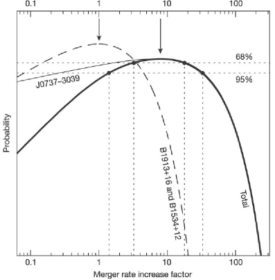
Figure 3: Probability density function (pdf) for the increase in the double–neutron–star merger rate resulting from the discovery of PSR J0737–3039. The dashed line represents the pdf corresponding to the old merger rate (before the discovery of PSR J0737–3039). The heavy solid line represents the pdf corresponding to the new merger rate (from new_NSNS ).

The remarkable weakness of PSR J0737-3039 radio signals, despite its relative nearness ($\sim 600$ pc) to Earth, further suggests that there might be a plethora of as yet undetected short-lived NS-NS binaries in the Galaxy. This is the dominant source of uncertainty in estimating NS-NS merger rates, which might accordingly be $\sim 10^{2}$ larger than estimated, as stressed in merger_rate4 , where it is argued that all other modeling uncertainties build up only to an uncertainty factor of the order of unity.

In order to translate the above event rates into observable event rates, one has to estimate the visibility distance of the MAGO detector. We define here the visibility distance as the distance of a source yielding SNR$=1$.

To determine the visibility distance of MAGO (and/or a MAGO array, or xilophone), one may adopt the std. (conservative) procedure appropriate for the case where detailed knowledge of the waveform is not available. One accordingly has to compare the squared sought signal characteristic amplitude,

$$h^{2}_{c}=\frac{2}{\pi^{2}r^{2}}\frac{dE}{df}$$

to the squared detector’s r.m.s. noise ampltude,

$$h^{2}_{n}=\frac{fS(f)}{\langle F^{2}\rangle}$$

so as to recast the signal to noise ratio into the form

$$\mathrm{SNR}=\left[\int d(\log f)\frac{h^{2}_{c}(f)}{h^{2}_{n}(f)}\right]^{1/2}$$

where $S(f)$ is the detector noise power spectral density (PSD), $F$ is the detector’s directivity function, $\langle\cdot\rangle$ denotes averaging over all directions, and $dE/df$ describes the spectral energy content of the sought signal. Based on reasonable assumptions about the transition from inspiral to merger, we might use for this latter the formula (in geometrized units)

$$\frac{dE}{df}\sim\displaystyle{\left\{\begin{array}[]{l}0.91M^{2}\times\left(4\mu/M\right)^{2},~{}~{}~{}f\in(f_{merge},f_{ring})\\ 0,~{}~{}~{}\mathrm{elsewhere}\end{array}\right.}$$

first proposed in Flanagan , where $f_{merge}\sim f^{(GW)}_{LSCO}\sim 4\times 10^{3}(M_{\odot}/M)$ Hz and $f_{ring}\sim 2.6\times 10^{4}(M_{\odot}/M)$ Hz is the quasi-normal mode ring-down frequency of the final collapsed object Flanagan .

For a medium-size MAGO ($S_{h}^{1/2}\sim 6\times 10^{-21}$ Hz^-1/2 @ $2$ KHz in a $350$ Hz bandwidth) the corresponding visibility distance (SNR$=1$) will be $\sim 0.2$ Mpc for a $M\sim 10M_{\odot}$ merger with a sharp cut–off at $M\sim 2M_{\odot}$. With a MAGO xylophone covering the 2–8 KHz band at the same PSD level, the mass range could be extended down to $M\sim 0.6M_{\odot}$. (see fig. 4).

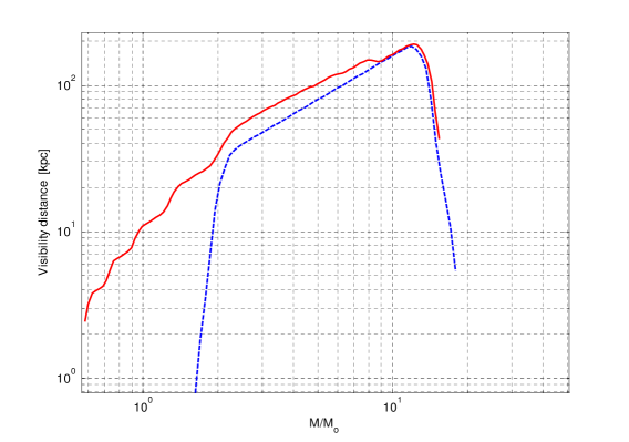
Figure 4: Visibility distance of one MAGO (dashed line) and of a xylophone of six MAGOs covering the 2–8 kHz frequency range (solid line) vs. total mass of the merger (in solar mass units).

III.2 Bursts

The characteristic noise amplitude of one MAGO is $h_{n}(f_{c})\sim 7\times 10^{-19}$ at the characteristic frequency $f_{c}\sim 2$ kHz. This accounts for the isotropic conversion into GW energy of $8\times 10^{-4}$ solar masses located at a distance of 8 kpc (SNR=1) (see fig. 5).

Recently pizzella a coincidence excess was found among the data of the resonant bars EXPLORER and NAUTILUS, when the detectors are favorably oriented with respect to the galactic disk. The observed coincidence corresponds to a conventional burst with amplitude $h_{c}\sim 2\times 10^{-18}$ and to the isotropic conversion into GW of $4\times 10^{-3}M_{\odot}$, with sources located in the Galactic Center. Still unknown phenomena other than GWs, though, cannot be ruled out as causes of the observed events pizzella . A possible way to distinguish GWs from other sources is the use of several, different, detectors with good sensitivity. From this point of view the use of a network of MAGOs could contribute in clarifying this subject.

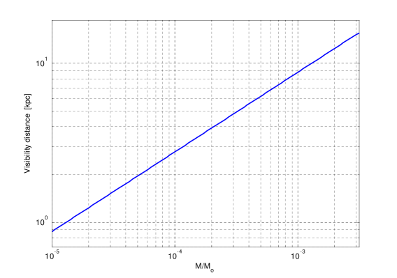
Figure 5: Visibility distance of one MAGO vs. burst energy (in solar mass units).

III.3 MACHO Binaries

The gravitational wave frequency corresponding to the last stable circular orbit, loosely marking the transition from inspiral to plunge in binary coalescence, is roughly Finn_vis :

$$f^{(GW)}_{LSCO}\sim 3976\frac{M_{\odot}}{M}~{}[\mathrm{Hz}]$$ (2)

for a (symmetric, non spinning, circular orbit) binary with total mass $M$.

The spectral window of MAGOs would thus be highly appropriate to observe gravitational waves from black-hole MACHO binaries MACHOs with a typical total mass of $0.6M_{\odot}\lesssim M\lesssim 2M_{\odot}$. It is speculated MACHOs2 that one half of the galactic halo mass (corresponding to $\sim 3\times 10^{11}M_{\odot}$) consists of MACHOs with a typical mass of $M\sim 0.3M_{\odot}$. Among these, $\sim 30\%$ should be bound in binary systems, formed at the same time ($10^{10}$ yr) the galaxy was born and uniformly distributed across the halo. The rate of MACHO binary coalescence could be of the order of $10$ events per year acu_Finn in the galactic halo.

A nice representation of current expectations for BH–MACHO binary inspiral (and merger) observable event rates has been recently given by J.C.N. de Araujo and co–workers MACHO_Brazil for the (advanced) Brazilian spherical antenna ”Mario Schenberg” as a function of the burst sensitivity, and is shown in fig. 6. The burst sensitivities $h$ in fig. 6 are readily translated into visibility distances $d$ by noting that $h(d_{1})/h(d_{2})=d_{2}/d_{1}$.

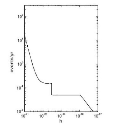
Figure 6: BH–MACHO binary inspiral (and merger) observable event rates for the (advanced) Brazilian spherical antenna ”Mario Schenberg” as a function of the burst sensitivity (from MACHO_Brazil ).

For visibility distances up to the Galaxy’s border ($d\sim 20$ Kpc) the event rate increases linearly up to $\sim 0.05$ yr^-1. This accounts for the linear segments on the right side of fig. 6. From the border of the Galaxy up to the outskirts of $M31$ and $M32$, at $d\sim 700$ Kpc, intergalactic BH–MACHOs might be visible. Their contribution, however, would be negligible under the assumption that they follow the distribution of dark matter. This corresponds to the plateau in figure 6. As the visibility distance overpasses $M31$ and $M32$, the event–rate contribution of these latter is added, corresponding to the step in fig. 6. For larger distances, beyond $1$ Mpc, the background BH–MACHOs contribution to the event rate becomes eventually dominant. The relevant event–rate is obtained using the coalescency rate computed in BHMACHO_Nakamura (leftmost region in fig. 6).

The visibility distance (SNR=1) for observing a coalescing $0.5M_{\odot}+0.5M_{\odot}$ MACHO binary with a MAGO ($S_{h}^{1/2}=6\times 10^{-21}$ between $1850$ Hz and $2150$ Hz) would be $\sim 18$ kpc. The maximum visibility distance for this detector is 25 kpc for observing a $0.9M_{\odot}+0.9M_{\odot}$ MACHO binary.

Furthermore, in view of MAGO’s relatively simple, lightweight and hopefully cheap features, one might think of building arrays of many MAGOs, either identical or differently tuned detectors (xylophone) whose response would allow to deduce the relevant source parameters (chirp-mass etc.). Fig. 7 shows the visibility distance of both six identical MAGOs as a function of the binary total mass.

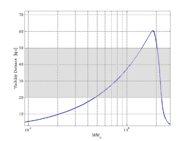
Figure 7: Visibility distance of an array of six identical MAGOs vs. the binary total mass. The typical distance of the galactic halo is also shown (gray area).

III.4 Submillisecond Pulsars

The existence of sub-millisecond pulsars has been speculated by various Authors. It is well known that the (lower) limiting spin period of a neutron star depends on the assumed equation of state, being $\sim 600\,\mu\mathrm{s}$ for the softest one breakup . Submillisecond pulsars, if any, could be strange (quark) stars quark as well. Known millisecond pulsars are believed to be ”recycled” neutron stars spun-up by accretion from the companion, in low-mass X-ray binary systems (LMXB) spinup . On the other hand, the so called gravitational radiation induced Rossby(r)-mode instabilities rmode are now believed to play a crucial role in setting an upper limit to the spin period Arras . As a matter of fact, the distribution of periods of all known pulsars drops off quite sharply at about $2$ msec. All sub-millisecond pulsar search campaigns made so far have been indeed negative submill1 , submill2 . Under such circumstances the possible direct observation of gravitational radiation from pulsars above $2$ KHz appears to be extremely difficult, though it cannot be completely ruled out.

III.5 Stochastic Background

The standard procedure to search for a stochastic background of gravitational waves (unresolved superpositions of gravitational wave signals of astrophysical or cosmological origin) is to cross-correlate (and suitably filter) the data of two (or more) detectors

Specific strategies for GW background detection using two bar detectors twobars , two spheres twoballs , two interferometers twoligos , a bar and an interferometer mixed have been discussed by various Authors, and are in current use to set upper limits on the gravitational wave background power spectral density on the basis of available data from operational gravitational wave antennas Whelan –Abbott .

We plan to develop a similar (straightforward) analysis for the special relevant cases of two MAGOs, one MAGO and one bar (or sphere), and one MAGO and one interferometer.

In view of the easy tunability of MAGOs at any frequency in the range between $10^{3}$ Hz and $10^{4}$ Hz and beyond, using MAGOs might be interesting for probing the otherwise unaccessible high frequency part of the sought stochastic gravitational wave spectrum.

IV Detector Layout

IV.1 Electromagnetic design

In order to build an efficient detector, a suitable cavity shape has to be chosen. According to some general considerations, a detector based on two coupled spherical cavites looks very promising (Fig. 1) rfsc01 . The choice of the spherical geometry is based on several factors. From the point of view of the electromagnetic design the spherical cell has the highest geometric factor $G$, thus it has the highest electromagnetic quality factor $\cal{Q}$, for a given surface resistance $R_{s}$ (${\cal{Q}}=G/R_{s}$). For the TE₀₁₁ mode of a sphere, the geometric factor has a value $G\approx 850\,\Omega$, while for standard elliptical radio-frequency cavities used in particle accelerators, the TM₀₁₀ mode has a value $G\approx 250\,\Omega$. Looking at the best reported values of surface resistance of superconducting accelerating cavities, which typically are in the $10^{-8}\,\Omega$ range, we can extrapolate that the electromagnetic quality factor of the TE₀₁₁ mode of a spherical superconducting cavity can be ${\cal{Q}}\approx 10^{10}-10^{11}$.

In the first generation of detectors, dedicated to the development of the experimental technique, the internal radius of the spherical cavity will be $r\approx 100$ mm, corresponding to a frequency of the TE₀₁₁ mode $\omega\approx 2$ GHz. The overall system mass and length will be $M\approx 5$ kg (with a wall thickness $w\approx 2$ mm) and $L\approx 0.5$ m. The choice of the wall thickness is made considering both practical and design constraints. On one hand, the wall thickness should be kept small enough to allow an easy fabrication while maintaining sufficient stiffness to withstand the external pressure once the cavity is evacuated. Furthermore, wall thickness was chosen to optimize the cavity cooling process, and to guarantee optimum stability against point–like thermal dissipation due to possible defects present on the cavity inner surface. On the other hand, wall thickness can be used to design a particular mechanical resonant frequency and it is obviously related to the mass of the detector, which plays an important role in the signal to noise ratio.

Since this type of detector is ideally suited to explore the high frequency region of the g.w. spectrum, we plan to build a tunable cavity with $4$ kHz$\leq\omega_{2}-\omega_{1}\leq 10$ kHz, which is outside the spectral region covered by the resonant and interferometric detectors, both existing and planned, and is still in a frequency region where interesting dynamical mechanisms producing g.w. emission are predicted schutz2003 ; grqc0109054 ; kokko2 .

The interaction between the g.w. and the detector is characterized by a transfer of energy and angular momentum. Since the helicity of the g.w. (the angular momentum along the direction of propagation) is $2$, the g.w. can induce a transition between the two levels provided their angular momenta differ by $2$; this can be achieved by putting the two cavities at right angle or by a suitable polarization of the electromagnetic field inside the resonator. The spherical cells can be easily deformed in order to induce the field polarization suitable for g.w. detection. The optimal field spatial distribution has the field axes in the two cavities which are orthogonal to each other (Fig. 8). Different spatial distributions of the e.m. field (e.g. with the field axes along the resonators’ axes) have a smaller effect or no effect at all.

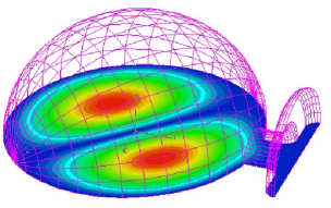
Figure 8: Electric field magnitude of the TE₀₁₁ mode. Note the alignment of the field axis

A tuning cell is inserted in the coupling tube between the two cavities, allowing to tune the coupling strength (i.e. the detection frequency) around the design value. The dependence of the detection frequency on the distance between the two coupled cells is shown in Fig. 9, while its dependence on the diameter of the tubes is shown in Fig. 10.

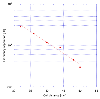
Figure 9: Detection frequency vs. coupled cells distance

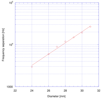
Figure 10: Detection frequency vs. coupling tubes diameter

One detector based on two spherical niobium cavities (with fixed coupling) has recently been built and tested at CERN. A second detector with variable coupling has also been built and is now being tested (Fig. 2).

The first test on the cavity with fixed coupling, showed a quality factor ${\cal{Q}}\geq 10^{10}$ (see Fig. 11). This corresponds to a surface resistance $R_{s}\approx 50$ n$\Omega$, a factor of ten higher than the best values reported for superconducting accelerating cavities. The obtained result is very satisfactory. In fact, the whole fabrication procedure (including surface treatments) is optimized for the elliptical cavity geometry used for high energy particle acceleration. Some development is still needed to tailor the technique to the spherical shape of our resonator and to obtain a surface quality comparable to that routinely obtained on elliptical cavities that would lead to a quality factor ${\cal{Q}}\approx 10^{11}$.

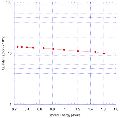
Figure 11: Quality factor vs. stored energy for the fixed–coupling cavity

IV.2 Mechanical design

From the mechanical point of view it is well known that a spherical shell has the highest interaction cross-section with a g.w. and that only the quadrupolar mechanical modes of the sphere do interact with a gravitational wave lobo . The mechanical design is highly simplified if a hollow spherical geometry is used. In this case the deformation of the sphere is given by the superposition of just one or two normal modes of vibration and thus can be easily modeled. In fact, the proposed detector acts essentially as an electro–mechanical transducer; the gravitational perturbation interacts with the mechanical structure of the resonator, deforming it. The e.m. field stored inside the resonator is affected by the time–varying boundary conditions and a small quantity of energy is transferred from an initially excited e.m. mode to the initially empty one. We emphasize that our detector is sensitive to the polarization of the incoming gravitational signal. Once the e.m. axis has been chosen inside the resonator, a g.w with polarization axes along the direction of the field, will drive the energy transfer between the two modes of the cavity with maximum efficiency. With standard choices for the axes and polar coordinates, the pattern function of the detector is given by $F_{\times}=-\cos(\theta)\sin(2\phi)$, and is equal to the pattern function of one mechanical mode of a spherical resonator.

IV.3 Status and results on the simulation of the mechanical modes

We have run an ANSYS mechanical simulation of our prototype over a wide frequency range ($0$–$7000$ Hz), finding approximately 180 resonant modes and we have compared these modes to the (analytical) modes of a spherical shell for identification.

We foresee to suspend the detector by a region near its center of mass, a region where the tuning system should also be implemented. For this reason, the model used for the simulation consists of half detector (single cell) fixed on the central pipe, near the whole detector center of mass. Let us focus on two frequency ranges: the modes below the quadrupole frequencies (ANSYS calculated $\nu_{quad}=3646$ Hz, theoretical frequency is $\nu_{quad}=3750$ Hz) and the modes above $\nu_{quad}$.

Below $\nu_{quad}$, we find a very limited number of modes ($\sim 16$), well separated in frequency. These modes are due to the movement of the pipes with respect to the cavity (bending, rotation and cantilever modes). Above $\nu_{quad}$ we find a great number of modes, only related to the cell. Fig. 12 shows the cumulative number of modes versus their frequency. The slope of the ANSYS calculation (blue dots) is very close to the slope of the analytical spherical modes (green cross), meaning that the number of the single cell modes found above $\nu_{quad}$ corresponds to the ideal sphere, although several mode shapes may be distorted due to the presence of the pipes.

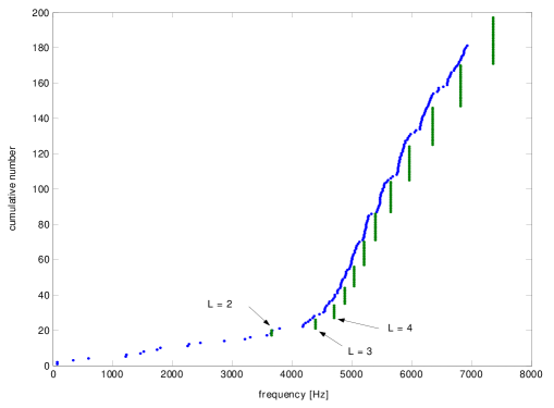
Figure 12: Spectrum of the mechanical normal modes of the small–scale detector in the range $0<f<7000$ Hz.

The frequency range around the quadrupolar mode of interest ($N$,$L$,$M$ = 1,2,2) gives us two main hints:

• The rightfulness of the detection mode, which is minimally perturbed by the pipes attached to the cavity and oscillates approximately at the wanted frequency;

• The presence of only quadrupolar modes in the range of interest.

The first quadrupolar mode resembles one of the fundamental quadrupole mode of a single, ideal sphere. The five quadrupolar modes are all near to each other, although the cavity pipes interference gives a discernible spread. A visual identification with the ideal spherical modes can be done for the $L=2$, $L=3$ and $L=4$ mode groups. Higher order modes, although somewhat similar to the ideal case, are in general less easy to identify.

IV.3.1 Role of other mechanical mode scarce

Consider now a detector tuned to an angular frequency $\Omega=\omega_{2}-\omega_{1}$ and let us focus on OMR operation, so that $\Omega>\omega_{mech}$. The signal, driven by the gravitational wave, comes from the quadrupolar modes (in particular, for a well oriented source, from the $N$,$L$,$M$ = 1,2,2 mode). That is, the gravitational wave couples to those modes, driving them at angular frequency $\Omega$. The thermal noise, which will surely come at least from the same quadrupoles, may in principle come from other mechanical modes. In particular, we seek deformations which contribute to the noise but are not affected by the signal (g.w.). For a mode to contribute to noise sources though, it must fulfill two stringent requirements:

• The coupling coefficient $C_{m}^{21}=\int_{S}\left(\mathbf{H}_{2}\cdot\mathbf{H}_{1}-\mathbf{E}_{2}\cdot\mathbf{E}_{1}\right)\mathbf{\xi}_{m}\cdot\,d\mathbf{S}$, between the electromagnetic modes and the mechanical mode must not be null;

• The mode frequency must be relatively near to the detection frequency.

The first requirement is the most important.

In the ideal, spherical case, the coupling coefficient $C_{m}^{21}$ is different from zero for the class of quadrupole modes alone. Other angular numbers exhibits a strictly zero coefficient due to symmetry mismatch between the electromagnetic field and the mechanical mode.

A clue for this behavior comes from the chosen electromagnetic mode angular dependence, which is $\propto\cos{(2\theta)}$ (it is not depending on $\phi$), while the radial component of the displacement is proportional to $\cos{(L\theta)}$. This calculation has been performed on an ideal, hollow sphere and using analytical expressions for the electromagnetic fields. We understand that these results must be checked against the more realistic deformations delivered by ANSYS, and our future efforts will surely tackle this problem. We are confident though that the general behavior will be consistent, since the preliminary analysis shows a considerable similarity between sphere modes and the ANSYS model.

V Suspension System

Like a resonant bar, the whole detector must be thoroughly insulated from the environment and the mechanical design of the insulation is therefore strongly bonded with the cryogenic design. In particular, the insulation for the direct LHe supply to the cavity (see section VI) may prove to be a formidable task. The mechanical insulation foreseen for this detector may be inspired by the already existing resonant bars suspension systems, although some major differences exist.

Since one of the feature of this detector is the tunability, the mechanical design should provide adequate insulation in the frequency range 4–20 KHz and a very rough estimation suggests a minimum value of $250$ dB of attenuation in the desired band (by comparison, Al bars suspension are estimated to provide $\approx 300$ dB of insulation). A sketch of the suspension system is shown in fig. 13.

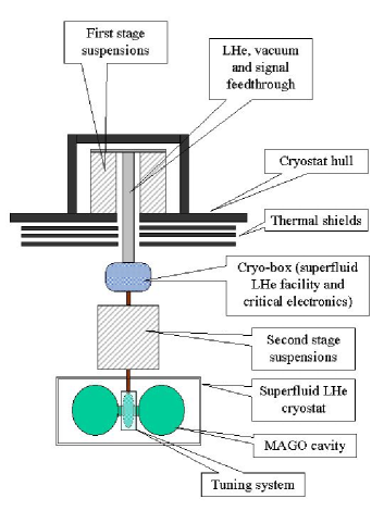
Figure 13: Sketch of the suspension system

The room temperature filter bank is attached to the outer cryostat hull and will provide a first decoupling to the environment. There follows a cryogenic box, a facility which will host some critical low-temperature electronic components and the source for the superfluid LHe, and finally the cryogenic filter bank, which should provide the required insulation. This second stage filter is connected to the innermost cryostat, which is a superfluid LHe container hosting the detector and its tuning system. The non trivial task of filtering out environmental acoustical noise on a wide frequency band can be more easily accomplished by optimizing the two filter banks on separate frequency ranges, for example, the first stage can be optimized for low frequencies. The effectiveness of the cold filter (second stage) can be weakened by the superfluid LHe feedthrough, which runs from the cryogenic box to the MAGO cavity cryostat. Although the superfluid LHe can be conveyed by means of a suitable capillary tube, acoustic vibrations in LHe, triggered in cryo-box for instance, require a deeper understanding and maybe a dedicated damping system. The mechanical insulation design is made more complex by the MAGO cavity plus the superfluid cryostat weight. Since their weight is of the order of some tens of kilos, it is comparable to the suspensions weight and therefore, the load on uppermost suspension element can be considerably different from the lowermost one. All these problems will be addressed in the following years, where a comprehensive cryogenic and mechanical design will constitute the main effort.

V.1 Seismic Noise

Preliminary seismic noise measures have been performed in our laboratory during working hours (day time). The measures were taken in a range from 10 to 9000 Hz, which should cover the sensitive region for the MAGO detector. By comparing the data to the expected level of the thermal noise we can estimate the required attenuation of the external environment noise to be (at least) of the order of 180–200 dB in the range 500 Hz–9 kHz, and 160 dB if we limit the frequency range to $f>4$ kHz.

V.1.1 Data taking

Seismic noise was acquired with a PCB 393B12 accelerometer connected to a Stanford research SR780 FFT analyzer. The accelerometer has a nominal frequency range of 0.05 to 4000 Hz and a sensitivity of 1019.4 mV/(m/s²). Although that particular accelerometer is not fit for measuring frequencies up to 9000 Hz, we have nevertheless taken the frequency range 10–9000 Hz in order to have a preliminary, order of magnitude measure of the environmental disturbances in the range of interest. We are justified in taking the high frequency measures because the accelerometer response has a rising characteristic with increasing frequency (ref. model 393B12 operating guide). It is thus expected that the high frequency portion of the seismic noise power spectral density might be overestimated. More accurate evaluation of the seismic noise in the high frequency range ($f>4000$ Hz) will be done as soon as our group is provided with a suitable accelerometer (for instance the PCB 307B).

The accelerometer was secured to a 25 kg lead brick, which allowed us to easily sample the vibrations along the three orthogonal directions in space, defining axis $z$ oriented perpendicular to the floor, whereas $x$ and $y$ parallel to the room walls. For each direction, a measure with the accelerometer switched off (null measure) was performed in order to take into account the SR780 FFT and cables intrinsic noise over the whole frequency range.

The sub–cooled liquid helium environment, needed for MAGO operation, is provided by means of a big mechanical pump, located next to the laboratory. When switched on, this pump emits an audible noise, and for this reason measures were taken with the pump both switched on and off.

The Volts measured as the output of the accelerometers were converted into the equivalent force acting on our detector. This allows direct comparison with the Langevin force spectral density and therefore yields immediately the required attenuation. Sticking to a conservative approach, we have assumed that the noises measured in the three directions equally couple to the detector.

V.1.2 Results

Figure 14 shows the total force spectral density (summed over $x$, $y$ and $z$) with the helium pump switched on and off. The contribution of the pump is relevant up to a frequency $f\sim 3$ kHz.

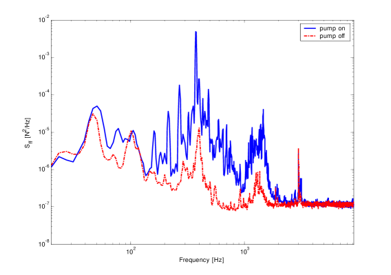
Figure 14: Total force spectral density measured in the ”quiet” condition (helium pump switched off, dotted line) and ”noisy” condition (helium pump switched on, continuous line).

If we require that the measured force spectral density be of the same order of the Langevin force spectral density $S_{ff}=4K_{b}TM\omega_{m}/Q_{m}$ , we immediately can calculate the approximate attenuation for the range of frequencies greater than a chosen cut off frequency $f>f_{0}$ (see fig. 15).

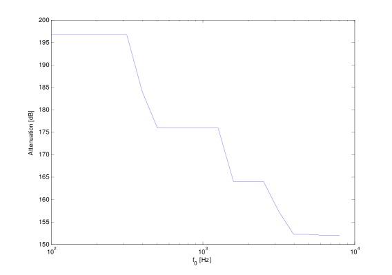
Figure 15: Minimum attenuation as function of the cut–off frequency $f_{0}$.

Although these measures are not conclusive, we expect the attenuation values proposed in this document to be a fairly good approximation. More accurate and reliable numbers could be provided with suitable test equipments and a setup nearer to a g.w. detector experiment. Note that the assumption of equal coupling between the vibrations in the three directions and the system may well be an overestimation of the real case. Further studies could therefore relax the attenuation requirements.

VI Cryogenics

Assuming the conservative value of 1 W/m² for the super–insulation radiation losses, the radiating heat load is $P_{rad}\approx 4$ W. Adding to this figure a couple of watts to account for the conduction losses in the cavity suspension (tie–rods), we obtain the value of $P_{tot}\approx 6$ W as an upper limit. These steady state losses have to be compared with the RF cryogenic losses of our detector.

Assuming, in operation, a peak surface magnetic field $H_{surf}=0.1$ T (half of the critical field of niobium) the stored energy in the cavity will be $U\approx 30$ J. We remark that $H_{surf}=0.1$ T corresponds (in an accelerating cavity) to 25 MV/m of accelerating field, a value routinely achieved in the cavities developed for the Tesla project. Given the geometric factor of our cavity, $G=$ 835 $\Omega$, and assuming a residual surface resistance of 5 n$\Omega$ (the surface resistance routinely obtained in the LEP–II cavities at 1.8 K), we can foresee a quality factor ${\mathcal{Q}}\approx 10^{11}$, corresponding to a dissipation of 4 W in the helium bath (@ $H_{surf}=0.1$ T).

The planned operating temperature of our system is 1.8 K to fully exploit the advantages of the RF superconductivity. At the chosen frequency of 2 GHz the surface resistance at 1.8 K is well saturated at the residual value, avoiding the change of surface resistance produced by the heating of the surface. The use of superfluid helium as refrigerant guarantees a very good thermal dissipation for the cavity, with an even temperature distribution along the cavity surface.

To further improve the heat exchange and reduce the effect of the helium boil–off we propose a scheme of refrigeration similar to the one foreseen for the LHC magnets and already used since the eighties for the refrigeration of high field magnets (e.g. TORE–II supra). The flow chart of the refrigerator is shown in figure 16.

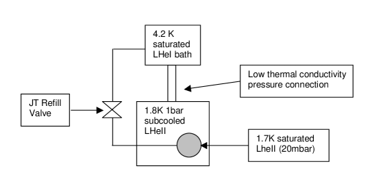
Figure 16: Flow chart of the subcooled superfluid helium refrigerator

This refrigeration scheme, using subcooled superfluid helium, at atmospheric pressure and 1.7–1.8 K, avoids all the problems related to the bubbles in the refrigerating bath, improves the Kapitza resistance at the helium–cavity wall interface and increases by 30% the peak transfer value to the helium bath. This refrigeration scheme will be the best solution also from the point of view of the mechanical noise induced on the detector by the LHe bath. The subcooled operation at 1.8 K and atmospheric pressure (compared with saturated helium at 1.8 K and 20 mbar), will eliminate the possibility of the bubble gas production. This effect of an abrupt reduction of the bath induced mechanical noise below the helium $\lambda$–point was already experienced on Weber type gravitational detectors fulvioricci .

To form a bubble of a certain size in subcooled helium we need not only to transfer to the helium bath the amount of heat corresponding to the heat of vaporization, but also the enthalpy needed to reach the normal boiling point of the gas at 4.2 K. Furthermore the Claudet–type refrigerator reduces to a minimum the refrigerator–bath interaction minimizing the mechanical noise coming from the pumps and from the saturated HeI bath. The sub–atmospheric HeII bath cools the main bath only by conduction via the heat exchanger HT, the refill of this bath is done trough the JT needle valve working on the liquid helium flow. The hydraulic impedance of this needle is quite high and damps any pressure fluctuation due to the pumping system. The 4.2 K bath is in hydraulic contact with the 1.8 K sub–cooled bath via the high impedance duct to reduce the heat input to the superfluid helium and allows to reduce the bath temperature well below the $\lambda$–point of the helium (2.19 K). To obtain this result we need a quite long and narrow hydraulic channel with a very high thermal impedance, but also the hydraulic impedance of the channel is high, decoupling the superfluid bath from the saturated (4.2 K) or nearly superfluid bath. In this way pressure fluctuations due to the He bath refilling or to turbulences, produced by thermo–acoustic oscillations of the saturated bath, will have a negligible effect on the superfluid bath.

Coming to the conclusions the proposed refrigeration scheme will greatly help in reducing the sensitivity of the proposed detector to the acoustic noise produced by the fluctuation of the helium bath wile giving us the more comfortable situation by the point of view of the RF performances.

VI.1 Refrigeration scheme and Noise Issues

The microwave power dissipation in the cavity walls is easily found by the quality factor definition

$$Q=\frac{\omega U}{P}$$ (3)

with $\omega$ angular frequency of the radio–frequency (RF) field, $U$ Electromagnetic energy stored in the resonator, and $P$ RF power lost in the cavity wall.

In our case (operating frequency $\omega\sim 2$ GHz) for a stored energy $U\sim 18$ J, corresponding to cavity operation at peak surface magnetic field $B_{peak}\sim 100$ mT (already achieved on the prototype cavity measurements), the power dissipation is $P\sim 20$ W at the design electromagnetic quality factor $Q=10^{10}$. The measured quality factor for the prototype MAGO cavity is $Q=5\times 10^{10}$ at the design field, giving a safety factor of five over the power dissipation level quoted in the proposal.

The RF power dissipation is fairly constant on more than 70% of the resonator surface; moreover the temperature dependence of the RF surface resistance of the niobium is highly non linear bardeen58 , the thermal conductivity of the superconductor is very poor, and the heat capacitance low (zemansky, , chapter 15). For those reasons (for the quoted quality factor and field) the resonator can only be cooled via an helium bath.

Localized thermal connections to an heat sink at low temperature, as the one used for cooling bars, lead to thermal runaway of the resonator over the critical temperature of the niobium, up to 20 to 30 K. Considerations on the thermal noise of the detector, and the temperature dependence of the RF surface resistance of superconductors suggest to operate the detector at the lowest possible temperature. Practical considerations on readily available refrigerators with cooling power exceeding 10 watt, restrict our choice to a refrigerator scheme using superfluid helium operating around $T=1.5$–$1.8$ K.

At the operating temperature of $T=1.8$ K the largest practical superfluid helium refrigerators, designed for the operation of superconducting cavities, have a cooling power in the multi kW range and superfluid helium refrigerators developed for superconducting magnet operation have $\sim 10$ kW of refrigerating power claudet88a . The world largest dilution refrigerator, the Compass refrigerator at CERN, has a maximum cooling power of 1 W at 0.3 K and 10 mW at 80 mK berglund . Finally, considerations of sec. VI.2.2 on the impact of the coolant fluid on the mechanical quality factor of the resonator, strongly suggest to use as coolant superfluid helium at $T\sim 1.6$–$1.5$ K.

VI.1.1 Refrigerator Scheme

The proposed refrigeration system is a pressurized superfluid helium bath operating at $T=1.5$–$1.7$ K and $P=10^{5}$ Pa, based on the original Claudet system developed at CEA for the TORE II Supra superconducting Tokamak claudet88b . A conceptual design of the refrigeration system is shown in fig. 17.

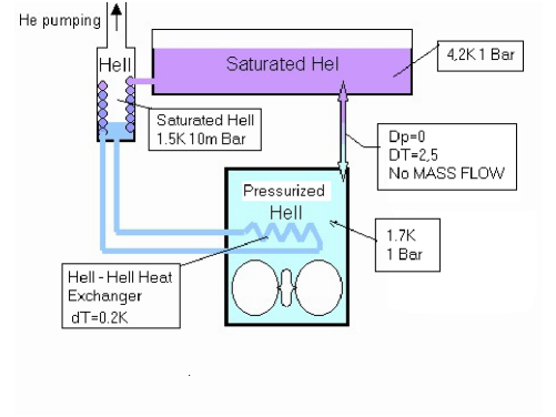
Figure 17: Pressurized Superfluid Helium (Claudet type) refrigerator.

The cavity is immersed in a pool of stagnant superfluid helium and is cooled by conduction (not convection) by the surrounding pressurized superfluid helium bath at $T=1.7$ K and $P=10^{5}$ Pa.

The operation of the cryostat is the following: the reservoir (housing the cavity) is filled with liquid superfluid helium at one bar. The superfluid helium in the reservoir is kept at $T=1.7$ K by the HeII–HeII heat exchanger cooled at 1.5 K by the saturated superfluid helium produced by pumping on the saturated HeII pot. The pressure on the reservoir is kept at one bar by the hydraulic connection (a narrow channel) with the saturated liquid helium (HeI) at one bar and 4.2 K. Inside this narrow channel lies the HeI–HeII interface with a temperature drop of 2.5 K, and no pressure drop because no liquid helium flow takes place in the channel.

The heat produced by the RF power dissipation on the cavity walls is transferred to the HeII–HeII heat exchanger by the large thermal conductivity of the superfluid helium. This large thermal conductivity, (together with the peculiar properties of the superfluid helium) keeps homogeneous the temperature of the refrigerant in the reservoir, preventing any convection in the liquid and the generation of any flow–induced noise in the reservoir. Moreover at the rated dissipation of 20 W, the power flow per unit area is roughly $10$ mW(cm)^-2, a factor of 100 lower than the value for the onset of bubble formation in the helium bath at the cavity surface. Roughly speaking, to produce bubbles in pressurized HeII one needs to transfer to the bath the extra energy needed to heat the liquid from 1.7 K to 4.2 K.

Both effects, tightly connected to the use of pressurized superfluid helium, will guarantee us against noise generation in the process of cavity refrigeration.

VI.1.2 Induced noise in the cavity reservoir

The proposed refrigeration scheme is quite safe in keeping to a minimum the noise generated from the thermal dissipation in the liquid helium bath. An additional source of acoustic noise is the pressure fluctuation in the helium reservoir.

Two main sources inducing acoustic waves in the helium are the pressure fluctuations on the saturated 4.2 K helium bath and pressure fluctuations induced by the pumping system on the saturated 1.5 K HeII pot feeding the HeII–HeII heat exchanger.

The pump–related pressure fluctuations on the HeII pot are decoupled from the pressurized HeII reservoir by the metallic wall of the heat exchanger. The two sections of the refrigeration system are only in thermal contact, but mechanically separated. Usually, the heat exchanger is a metallic box filled by the superfluid helium produced in the pot. Moreover the thermodynamic properties of the superfluid helium allow to relocate the saturated HeII pot far away and to feed the heat exchanger by mechanically decoupled lines (in the TORE Supra system the 1.5 K pot is roughly 10 meters apart from the heat exchanger) claudet88b .

The pressure fluctuation on the 4.2 K bath are also rejected by the system. The pressure connection between the pressurized superfluid reservoir and the saturated helium bath need to be kept as small as possible to improve the refrigerator efficiency.

We remind that no liquid helium flows trough the connections, and that the steady state heat input at the 4.2 K HeI–1.7 K HeII interface is produced by thermal conduction in the helium. This heat flow is proportional to the cross section of the interface: the smaller the channel, the better is the efficiency of the refrigerator. Usually [5] the pressure connection is a tiny tube of about 1 mm cross section or less. Pressure fluctuations in the saturated 4.2 K HeI bath are greatly reduced, at the superfluid helium side by the large hydraulic impedance of this channel.

The last source of noise in the helium bath is the background mechanical noise (seismic and man made) coupled to the liquid by the motion of the walls of the refrigerator. By this way the mechanical background noise can spoil the rejection of the mechanical–suspension attenuator bypassing the filter via the acoustic wave transmission of the liquid helium. To counter this effect we foresee the modification of the refrigerator outlined in fig. 18; the cavity helium II reservoir is hydraulically decoupled from the upper part of the pressurized HeII bath using an hydraulic low pass filter giving an attenuation of 200 dB at 4 KHz. The needed attenuation can be obtained using a 4 cell low pass filter with a cut–off frequency of $\sim 4$ Hz, producing an asymptotic attenuation of $\sim 60$ dB per cell at 4 kHz.

In this way all the mechanical noise, converted to acoustic wave in liquid helium, is confined in the upper reservoir. The upper reservoir is also the starting point of the last stage of the mechanical attenuator used to decouple the background mechanical noise from the active part of the detector (the resonant RF cavity) and can be (eventually) integrated with the mechanical filter.

The heat transport in the superfluid helium being given by thermal conduction, not by fluid convection, the only requirement on the hydraulic filter is to guarantee a mean cross section of the channel large enough to allow a temperature drop in the 0.1 K range (worst figure).

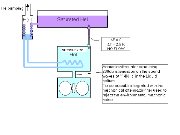
Figure 18: Modified refrigerator scheme including the hydraulic attenuator needed to decouple the detector from the mechanical noise converted to acoustic waves in the cooling bath.

VI.2 Mechanical dissipation in a liquid helium bath

The quality factor of a mechanical resonator is given by the ratio of the elastic energy stored in the mode of vibration and the power dissipated in one period:

$$Q=\omega\frac{U}{P_{diss}},$$ (4)

where $\omega$ is the resonant frequency. In vacuum, power can be dissipated only by the intrinsic losses of the resonator ($P_{intr}$) and the resulting intrinsic quality factor is defined as $Q_{0}=\omega U/P_{intr}$. For niobium at low temperature and few kHz, $Q_{0}\sim 10^{8}$.

If the resonator is immersed in a fluid, its oscillatory motion causes a periodic compression and rarefaction of the fluid near it, and thus produces sound waves. The energy carried away and dissipated by these waves is supplied from the kinetic energy of the body. Thus additional losses will be present and the quality factor will be given by:

$$Q=\omega\frac{U}{P_{intr}+P_{fluid}}$$ (5)

In a closed vessel only stationary sound waves can exist. For such waves three main dissipation mechanisms can be identified edmonds :

1. Power losses in the bulk of the fluid due to the classical processes of viscosity and thermal conduction:

   $$P_{bulk}=\frac{1}{2}\frac{\omega^{2}}{c^{2}}\left[\left(\frac{4}{3}\,\eta+\zeta\right)+\kappa\left(\frac{1}{c_{v}}-\frac{1}{c_{p}}\right)\right]\int_{V}u^{2}\,dV$$ (6)

2. Power losses in the viscous layer at the solid–fluid boundary, due to the tangential component of the fluid velocity at the boundary. The tangential fluid velocity should be zero at the wall, hence a tangential–velocity gradient must occur in the boundary layer of fluid, resulting in a viscous dissipation of energy:

   $$P_{visc}=\frac{1}{2}\left(\frac{\omega\rho_{0}\eta}{2}\right)^{1/2}\int_{S}(\mathbf{u}\cdot\mathbf{n})^{2}\,dS$$ (7)

3. Power losses in the thermal layer at the solid–fluid boundary. In a sound wave, in fact, not only the density and the pressure, but also the temperature, undergo periodic oscillations about their mean values. Near a solid wall, therefore, there is a periodically fluctuating temperature difference between the fluid and the wall, even if the mean fluid temperature is equal to the wall temperature. At the wall itself, however, the temperature of the wall and the adjoining fluid must be the same. As a result a temperature gradient is formed in a thin boundary layer of fluid. The presence of temperature gradients, however, results in the dissipation of energy by thermal conduction:

   $$P_{therm}=\frac{\rho_{0}^{2}c^{2}}{2p_{0}}\left(\frac{\omega\kappa}{2\rho_{0}c_{v}}\right)^{1/2}\frac{\gamma-1}{\gamma}\int_{S}u^{2}\,dS$$ (8)

Symbol	Property name
$\rho_{0}$	equilibrium density
$p_{0}$	equilibrium pressure
$c$	sound velocity
$u$	fluid velocity
$\eta$	shear viscosity
$\zeta$	kinematic viscosity
$\kappa$	thermal conductivity
$c_{v}$	specific heat at constant volume
$c_{p}$	specific heat at constant pressure
$\gamma$	specific heat ratio $c_{p}/c_{v}$

Table 1: Fluid properties and notation

The calculation of the total energy dissipated into the fluid requires the evaluation of the integrals over the fluid volume in eq. 6 and over the fluid–solid boundary in eq. 7 and eq. 8, which, in turn, depend on the details of the fluid velocity pattern. In the following section the calculation of the sound wave excited in a closed spherical vessel by an oscillating spherical shell is done.

VI.2.1 Forced fluid motion in a spherical vessel

The problem of the forced motion of a fluid in a closed (rigid) vessel can be analytically solved only in simple geometries. Here we shall focus on the problem of the calculation of the sound wave excited by an oscillating spherical shell of radius $a$ in a fluid which surrounds the shell and is enclosed in a spherical vessel of radius $R$ (see. fig. 19).

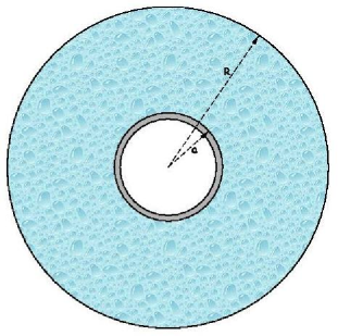
Figure 19: Sketch of the spherical shell (external radius $a$) enclosed in a concentric spherical vessel (radius $R$).

A sound wave is completely described by a scalar function $\phi(t,r,\theta,\phi)$ (the velocity potential) such that the velocity field is given by $\mathbf{u}=\mathbf{\nabla}\phi$. The mathematical problem can be casted in the following way: let us find the scalar function $\phi(t,r,\theta,\phi)$ which satisfies the wave equation (in spherical coordinates)

$$\nabla^{2}\phi-\frac{1}{c^{2}}\frac{\partial^{2}\phi}{\partial t^{2}}=0$$ (9)

and the boundary conditions:

$$(\mathbf{\nabla}\phi\cdot\mathbf{n})|_{a} = u_{0}f(\theta,\phi)$$ (10)

$$(\mathbf{\nabla}\phi\cdot\mathbf{n})|_{R} = 0$$ (11)

If we seek a solution of the wave equation for the velocity potential which is periodic in time, having the form: $\phi(t,r,\theta,\phi)=\phi_{0}(r,\theta,\phi)\exp{(-i\omega t)}$, then we find for $\phi_{0}$ the equation:

$$\nabla^{2}\phi_{0}+k^{2}\phi_{0}=0$$ (12)

where $k^{2}=(\omega/c)^{2}$. The most general solution of eq. 12 is given by the function

$$\phi_{0}=\sum_{l=0}^{\infty}\sum_{m=-l}^{l}R_{l}(r)Y_{l}^{m}(\theta,\phi)$$ (13)

where $Y_{l}^{m}(\theta,\phi)$ are the spherical harmonics, and $R_{l}(r)$ satisfies the Bessel equation

$$R_{l}^{\prime\prime}+\frac{2}{r}R_{l}^{\prime}+\left(k^{2}-\frac{n(n+1)}{r^{2}}\right)R_{l}=0$$ (14)

which has solutions:

$$R_{l}(r)=\frac{A_{l}J_{1}(l+\frac{1}{2},kr)+B_{l}J_{2}(l+\frac{1}{2},kr)}{\sqrt{r}}$$ (15)

where $J_{1}$ and $J_{2}$ are the Bessel functions of the first and second kind.

If we suppose that the vibrating spherical shell oscillates with quadrupolar pattern ($l=2$, $m=2$), so that the boundary condition at $r=a$ can be put in the form $(\mathbf{\nabla}\phi\cdot\mathbf{n})|_{a}=u_{0}Y_{2}^{2}(\theta,\phi)$ we get the following solution for the sound wave induced in the fluid:

$$\phi_{0}(r,\theta,\phi)=\frac{A_{2}J_{1}(\frac{5}{2},kr)+B_{2}J_{2}(\frac{5}{2},kr)}{\sqrt{r}}Y_{2}^{2}(\theta,\phi)$$ (16)

with the two constants $A_{2}$ and $B_{2}$ determined by the boundary conditions.

VI.2.2 Numerical estimates

Temperature	$T$	$1.5$ K
Pressure	$p_{0}$	$10^{5}$ Pa
Density	$\rho_{0}$	$1.47\times 10^{2}$ kg/(m3)
Shear viscosity	$\eta$	$1.5\times 10^{-6}$ kg/(m-sec)
Kinematic viscosity	$\zeta$	$1.5\times 10^{-5}$ kg/(m-sec)
Thermal conductivitya	$\kappa$	$0.1$ W/(m-K)
Specific heat (const. vol.)	$c_{v}$	$1150.3$ J/kg
Specific heat (const. press.)	$c_{p}$	$1151.1$ J/kg
Specific heat ratio ($c_{p}/c_{v}$)	$\gamma$	1.000695
First sound velocity	$c$	$242$ m/sec

Table 2: Physical properties of the liquid helium bath

Let us focus on a specific example. If we take the radius of the vibrating spherical shell $a=0.1$ m and the radius of the external vessel $R=0.3$ m, we get $Q\sim 10^{6}$, for a niobium sphere, oscillating at $f=4\times 10^{3}$ Hz (the frequency of the fundamental quadrupolar mode), in a bath of subcooled, superfluid helium at $T=1.5$ K and $P=10^{5}$ Pa. The physical properties used in the calculation are summarized in table 3.

External radius	$a$	$0.102$ m
Thickness	$w$	$2\times 10^{-3}$ m
Density	$\rho_{Nb}$	$8.6\times 10^{3}$ kg/(m3)
Mass	$M$	$2.2$ kg
Angular frequency	$\omega$	$2.5\times 10^{4}$ rad/sec
Intrinsic quality factor	$10^{8}$
Vessel radius	$R$	$0.3$ m
Helium volume	$V$	$0.1$ m3

Table 3: Characteristics of the small–scale system

For a large system ($a=0.6$ m, $R=1$ m), oscillating in the fundamental quadrupolar mode at $f=800$ Hz in a liquid helium bath with the same characteristics, we obtain $Q\sim 10^{7}$. The physical properties used in the calculation are summarized in table 4.

External radius	$a$	$0.6$ m
Thickness	$w$	$0.2$ m
Density	$\rho_{Nb}$	$8.6\times 10^{3}$ kg/(m3)
Mass	$M$	$5.5\times 10^{3}$ kg
Angular frequency	$\omega$	$5\times 10^{3}$ rad/sec
Intrinsic quality factor	$10^{8}$
Vessel radius	$R$	$1$ m
Helium volume	$V$	$3.3$ m3

Table 4: Characteristics of the large–scale system

Obviously, in addition to the mechanism of absorption which have already been considered, energy may also be lost from the sound field in the following ways:

1. by transmission of mechanical energy to the material of the vessel wall;

2. by subsequent radiation of energy from the outer surface of the vessel to the surrounding medium; This loss might be expected to acquire significance at resonant frequencies of the vessel;

3. by propagation of sound through the liquid helium tubing system.

These items need to be studied in detail on a realistic model of the whole cryogenic system and, at the end, will be the subject of experimental check.

VII Detection Electronics

The three main functions of rf control and measurement system of the experiment are:

1. The first task of the system is to lock the rf frequency of the master oscillator to the resonant frequency of the symmetric mode of the cavity and to keep constant the energy stored in the mode. The frequency lock of the master oscillator to the cavity mode is necessary to fill in energy in the fundamental mode of the cavity. The reduction of fluctuations of the stored energy to less than 100 ppm greatly reduces the possibility of ponderomotive effects due to the radiation pressure of the electromagnetic field on the cavity walls and helps to minimize the contribution of the mechanical perturbations of the resonator to the output noise. The frequency lock allows also to design a detection scheme insensitive to fluctuations of the resonant frequency of the two cavities forming our detector.

2. The second task is to increase the detector’s sensitivity by driving the coupled resonators purely in the symmetric mode and receiving only the rf power up–converted to the antisymmetric mode by the perturbation of the cavity walls. This goal can be obtained by rejecting the signal at the symmetric mode frequency taking advantage of the symmetries in the field distribution of the two modes. Our system, despite of some additional complexity, guarantees the following improvements over the one used in previous experiments:

   • a better rejection of the phase noise of the master oscillator obtained using the sharp resonance ($Q=10^{10}$) of the resonator as a filter;

   • a better insulation of the drive and detector ports obtained by using separate drive and detection arms of the rf system;

   • the possibility of an independent adjustment of the phase lag in the two arms giving a better magic–tee insulation at the operating frequencies;

   • a greater reliability for the frequency amplitude loop using the transmitted power, instead of the reflected, coming from the cavity.

3. The third task is the detection of the up–converted signal achieving the detector sensitivity limit set by the contribution of the noise sources bgpp2 . Slow pressure fluctuations on the cooling bath, hydrostatic pressure variations due to the changes in the helium level, pressure radiation, and so on, will change in the same way the resonant frequency of both modes. Using a fraction of the main oscillator power as local oscillator for the detection mixer, the detection system becomes insensitive to frequency drifts of both modes, allowing for a narrow band detection of the up–converted signal produced by the cavity wall modulation.

VII.1 The rf control loop

The RF signal generated by the master oscillator (HP4422B) is fed into the cavity through a TWT amplifier giving a saturated output of 20 Watt in the frequency range 2–4 GHz. The energy stored in the cavity is adjusted at the operating level by controlling the output of the master oscillator via the built–in variable attenuator.

The output signal is divided by a 3 dB power splitter. The $A$ output of the splitter is sent to the TWT amplifier, the $B$ output is sent, through the phase shifter (PS), to the local oscillator (LO) input of a rf mixer acting as a phase detector (PD). The output of the rf power amplifier is fed to the resonant cavity through a

double directional coupler, and a $180^{\rm o}$ hybrid ring acting as a magic–tee. The rf power enters the magic–tee via the sum arm, $\Sigma$, and is split in two signals of same amplitude and zero relative phase, coming out the tee co–linear arms 1 and 2.

The rf signal, reflected by the input ports of the cavity, enters the magic–tee through the co–linear arms. The two signals are added at the $\Sigma$ arm and sampled by the directional coupler to give information about the energy stored in cavity allowing for the measurement of the coupling factor, quality factor, stored energy. While driving the cavity on the symmetric mode no reflected signal is shown at the $\Delta$ port of the magic–tee where the signals coming from the co–linear arms are algebraically added to zero due to the $180^{\rm o}$ phase shift.

To get the maximum of the performances of the magic–tee we need to have equal reflected signals (phase and amplitude) at the cavity input ports. To preserve the signal integrity we use matched lines (in phase and amplitude) inside the cryostat. Because the phase shift is very sensitive to temperature inhomogeneities between the two cables and the phase difference between the two co–linear arms of the magic–tee gives a quite strong signal at the $\Delta$ port, we need to compensate for differential thermal contractions of the cables inside the cryostat, leading to phase unbalance in the feed lines. To do that we insert a phase shifter in one of the lines to compensate for differences and to reduce to a minimum the leakage of the unwanted modes on the two ports. As we will show in section VII.2, mode leakage of the symmetric mode to the $\Delta$ port sets a limit to the system sensitivity increasing the overall noise level of the detector.

Mode leakage of the antisymmetric mode to the $\Sigma$ port reduces the system sensitivity by reducing the signal level available for detection. The output ports of the cavity are coupled for a maximum output signal on the antisymmetric mode (detection mode) and the magic–tee is used to reject the rf power at the frequency of the symmetric mode. A fraction of the signal at the $\Sigma$ port is fed to the rf input of the phase detector PD via a low noise rf amplifier. The intermediate frequency (IF) output of the phase detector PD is fed back to the rf master oscillator to lock the output signal to the resonant frequency of the resonator. The total phase shift around the loop is set through the phase shifter PS, to have the maximum energy stored in the detector. A careful design of the servo loop amplifier (SLA) guarantees the stability of the system and the rejection of the residual noise of the master oscillator up to one MHz. The same fraction of the $\Sigma$ output of the output magic–tee is used to keep constant, to 100 ppm, the energy stored in the cavity feeding back an error signal to drive the electronically controlled output attenuator of the master oscillator.

Great deal of care is needed in tailoring the frequency response of both controls because the two loops can interact producing phase–amplitude oscillations in the rf fields stored in the cavities.

VII.2 Sensitivity enhancement using the mode symmetry

The two modes of the detector cavity have (as in the case of two coupled pendula) opposite symmetries of the fields.

Using two separate sets of ports to drive the cavity and to receive the up–converted signal at the frequency of the antisymmetric mode, the cavity acts as a very sharp filter (due to the high $Q$), with an high rejection of the noise coming from the master oscillator at the frequency of the up–converted signal. This already low residual noise, can be even more reduced in our scheme using two magic–tees to drive the cavity purely in the symmetric mode and to detect only the up–converted energy, rejecting the unwanted field components by an amount given by the magic–tee insulation.

In the case of an ideal magic–tee the mode rejection is infinite. If the cavity is driven purely in the symmetric mode no symmetric mode component is transmitted through the system and there will be no signal at the output port. In the ideal case this result is obtained also in the more simple scheme used by Melissinos and Reece rrm1 ; rrm2 , measuring the up–converted power coming out of the detector along the input lines.

Our scheme gives better sensitivity and performances in the real case. The first obvious gain is the sum of the $\Delta$ and $\Sigma$ port insulation of the two tees, plus the possibility of adjusting separately the input and output lines to get better mode rejection. In a commercial magic–tee the insulation is specified to be $\approx 25$ – $35$ dB over its own bandwidth. The reason for this quite low insulation is mainly due to the difficulty of balancing on a large range of frequency the phases of the signals coming from the two co–linear arms of the tee.

A phase unbalance as small as five degrees reduces the insulation from $\Delta$ to $\Sigma$ port to only 25 dB.

Our electronic scheme allows for an independent compensation of the magic–tee phase mismatch both at the feed frequency and at the detection frequency in a flexible way: the phase mismatch is compensated using a variable phase shifter at the input of one of the co–linear arms. The optimum phase at the input side results in a pure excitation of the symmetric (drive) mode, keeping the power at the frequency of the antisymmetric (detection) mode 70 dB below the level of the drive mode. Adjusting the phase at the output will couple only the antisymmetric mode component, rejecting the symmetric mode component by 70 dB. The total symmetric–antisymmetric mode rejection of the system is the sum of the attenuation we can obtain from the two $180^{\rm o}$ hybrids.

The input and output ports of the two cell cavity need to be critically coupled ($\beta$ = 1) to the rf source and to the rf detection system. In this way we have the optimum transfer of power to the symmetric mode (a maximum of stored energy) and to the antisymmetric mode (a maximum in the detector output). Because the frequency and field distribution of the two modes are quite close, the input and output ports are critically coupled to both modes. For that reason 50$\%$ of the symmetric mode signal is coupled to the idle $\Sigma$ port at the output magic–tee,

and symmetrically 50$\%$ of the antisymmetric mode signal is coupled to the idle $\Delta$ port at the input magic–tee. We remark that, since those two ports are not used in our detection scheme, it is necessary to reflect back into the cavity the energy flowing out of them. This task is achieved by a proper termination of the ports; a careful analysis showed that closing the ports with an open circuit completely decouples the input and output arms (optimum rejection of the symmetric mode) and maximizes the stored energy and the detector sensitivity.

At the $\Sigma$ port of the detection arm we insert a directional coupler to sample a tiny amount of the symmetric mode power coming from the cavity. This signal is fed into the frequency–amplitude servo loop used to lock the master oscillator to the cavity frequency and to keep constant the energy stored in the cavity.

VII.3 Detection of the converted signal

Having devised a means of suppressing the high level pump frequency signal, the remaining problem is to amplify and detect the low level parametric mode signal. The detection limit, hence overall sensitivity of the machine is now determined by the RF thermal noise level. In order to detect the low level signal it must be amplified and to do this without degrading the signal to noise ratio, a low noise amplifier is required. The lower the effective noise figure of the RF amplifier, the higher will be the sensitivity. In this case we can make use of the fact that the resonant cavities are operated at cryogenic temperatures and use a cryogenic low noise amplifier with lowest possible noise figure.

Since the late 1970s research has been conducted into the performance of GaAs FET and later GaAs HEMT RF amplifiers at cryogenic temperatures. The principle applications for this technology have been for radio astronomy receivers and for satellite ground station receivers. A typical receiver uses a 2 stage closed cycle Helium refrigerator reach a base temperature of around 15 K. HEMT amplifiers work well at this temperature if carefully design, but can also work down to liquid Helium temperatures. However, the additional benefit in noise temperature performance of operating at LHe compared to 15 K is not great and is mostly not justified when traded-off against of system complexity, when the equipment must operated in a radio astronomy telescope or a satellite ground station antenna. However, in this application, cooling to 4.5 K or 1.5K in liquid Helium is available in the same dewar as the superconducting coupled cavities.

The layout of the detection electronics is shown in fig. 20.

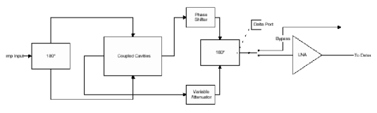
Figure 20: Electric circuit of the detector system

The signal converted to the antisymmetric mode by the interaction between the mechanical perturbation and the rf fields is coupled to the $\Delta$ port of the detection arm of the rf system and amplified by the low noise rf amplifier LNA.

The converted rf signal amplified by the LNA is fed to the rf input port (RF) of a low noise double balanced mixer M1; the local oscillator port (LO) of M1 is driven by the symmetric mode rf power (at angular frequency $\omega_{s}$). The LO input level is adjusted to minimize the noise contribution from the mixer. As shown in the previous section the input spectrum to the RF port of the mixer consists of two signals: the first at angular frequency $\omega_{s}$ coming from the rf leakage of the symmetric mode through the detection system; the second is the converted energy at angular frequency $\omega_{a}$. Both signals are down–converted by the M1 mixer giving to the IF port a DC signal proportional to the symmetric mode leakage and a signal at angular frequency $\Omega$ proportional to the antisymmetric mode excitation. The down–converted IF output is further amplified using a low noise audio preamplifier.

For the detection electronics of mechanically coupled interactions, at angular frequency $\Omega$, as gravitational waves, since the exact frequency and phase of the driving source is not known, we can’t perform a synchronous detection. We need to perform an auto–correlation of the detector output,

or to cross–correlate the outputs of two different detectors.

The outlined detection scheme gives the benefit of being insensitive to perturbations affecting in the same way the frequency of the two modes.

The first point to note in terms of the general architecture of the solution is that if a cryogenic amplifier is to be used within the same cryogenic dewar as the coupled cavities, then the phase shifter, variable attenuator and 180^o hybrid also need to be inside the dewar. If this is not the case then the noise temperature contribution of these components will dominate and there will be little, if any, benefit in having a cooled amplifier. As it is known that HEMT amplifiers can be produced for cryogenic operation, we shall first focus on the passive components. A consequence of placing the phase shifter and variable attenuator inside the cryogenic dewar is that they will have to be controllable by an electrical signal, rather than manually. For this reason the description below considers voltage controlled devices. In the interest of implementing a solution which is reasonably economic, the preferred approach will be to use commercial devices for the passive components, rather than developing special–to–type components. Many electronic components, particularly passive ones, will operate at cryogenic temperatures, even if not specified to do so by their manufacturers. Hence, the following focuses on the potential problems which will need to be investigated in order to qualify commercial components.

The 180^o hybrid is essentially a just a strip line device. The only concern about operation in cryogenic temperatures is due to differential thermal contraction of the materials of the component, particularly in the area of the connections between the strip line and coaxial I/O connectors. There may also be changes in dielectric properties of the substrate, which may affect the impedance of the I/O ports. Nevertheless strip line couplers have been used in many cryogenic applications without any problem, so we shall only validate this component with a simple test.

Voltage controlled phase shifter. The key element of the shift shifter is a varactor diode. Silicon and GaAs diodes are know to be capable of operation at cryogenic temperatures. However, particularly in the case of silicon, the electrical characteristics change significantly at cryogenic temperatures. Therefore, it is predicted that a phase shifter will still operate a cryogenic temperatures but its transfer characteristics will change significantly from the ambient temperature specifications. For this reason a particular aim will be to calibrate the device when operating at cryogenic temperatures. Another factor to note is that varactor diode phase shifters have limitations in operating power. Between 0 dBm and + 5dBm input power the varactor diodes begin to work as rectifiers. In any case, the pump energy in the cavity output ports is typically below 0dBm, but this should be confirmed.

Voltage controlled variable attenuator. The key element of a voltage variable attenuator is a diode and so the analysis given above for the phase shifter is also relevant for the variable attenuator.

Bypass Switch. The function of the bypass switch is to allow coarse tuning of the circuit for pump frequency suppression. Before the phasing is tuned the pump frequency signal may be large and could saturate the low noise amplifier. The bypass switch will allow for direct connection of a spectrum analyser outside the dewar for initial tuning. The bypass switch will be coaxial relay type.

VIII Response of the Detector

VIII.1 Signal

The interaction between the stored e.m. field and the time–varying boundary conditions depends on both how the boundary is deformed by the external perturbation and on the spatial distribution of the fields inside the resonator. Any field configuration inside the resonator can be expressed as the superposition of the electromagnetic normal modes slater : $\mathbf{E}(\mathbf{r},t)=\sum{\mathcal{E}}_{n}(t)\,\mathbf{E}_{n}(\mathbf{r})$; $\mathbf{H}(\mathbf{r},t)=\sum{\mathcal{H}}_{n}(t)\,\mathbf{H}_{n}(\mathbf{r})$, with ${\mathcal{E}}_{n}(t)\equiv\sqrt{\epsilon_{0}}\int\mathbf{E}\cdot\mathbf{E}_{n}\,dV$; ${\mathcal{H}}_{n}(t)\equiv\sqrt{\mu_{0}}\int\mathbf{H}\cdot\mathbf{H}_{n}\,dV$ and $\int\mathbf{H}_{n}\cdot\mathbf{H}_{m}\,dV=\int\mathbf{E}_{n}\cdot\mathbf{E}_{m}\,dV=\delta_{nm}$.

Similarly if $\mathbf{u}(\mathbf{r},t)$ denotes the displacement of the mass element of the walls at point $\mathbf{r}$ and time $t$, relative to its position at rest, the displacement of the walls can be written as the superposition of the mechanical normal modes $\bm{\xi}_{\alpha}(\mathbf{r})$ saulson : $\mathbf{u}(\mathbf{r},t)=\sum\bm{\xi}_{\alpha}(\mathbf{r})\,q_{\alpha}(t)$, with $\int\bm{\xi}_{\alpha}(\mathbf{r})\cdot\bm{\xi}_{\beta}(\mathbf{r})\rho(\mathbf{r})\,dV=M\delta_{\alpha\beta}$, where $M$ and $\rho$ are the mass and the density of the walls.

We want to study the energy transfer between two electromagnetic normal modes of a resonator whose boundary is perturbed by an external force when mode ”1” is highly excited by an external source at its eigenfrequency, ${\mathcal{H}}_{1}\approx A_{1}\cos(\omega_{1}t)$ and ${\mathcal{E}}_{1}\approx A_{1}\sin(\omega_{1}t)$, with constant amplitude $A_{1}$. We shall assume that only one mechanical mode couples to the external force. Including empirical damping terms, the equations of motion for the field amplitudes are given by:

$$\ddot{\cal H}_{2}+\frac{\omega_{2}}{\mathcal{Q}}\dot{\cal H}_{2}+\omega_{2}^{2}{\cal H}_{2}=-\frac{1}{2}\,\omega_{2}^{2}q_{m}C^{m}_{21}{\cal H}_{1}$$ (17)

$$\ddot{q}_{m}+\frac{\omega_{m}}{Q_{m}}\,\dot{q}_{m}+\omega_{m}^{2}q_{m}=\frac{f_{m}}{M}-\frac{1}{2}\frac{C^{m}_{21}}{M}\,{\mathcal{H}}_{2}{\mathcal{H}}_{1}^{*}$$ (18)

where $f_{m}(t)=\int\mathbf{f}(\mathbf{r},t)\cdot\bm{\xi}_{m}(\mathbf{r})\,dV$, and $\mathbf{f}(\mathbf{r},t)$ is the volume force density which acts on the walls. The time–independent coupling coefficient $C^{m}_{21}$ is given by (the superscript $m$ labels the mechanical normal mode, while the subscripts label the electromagnetic modes):

$$C^{m}_{21}=\int_{{S}}(\mathbf{H}_{2}\cdot\mathbf{H}_{1}-\mathbf{E}_{2}\cdot\mathbf{E}_{1})\,\bm{\xi}_{m}\cdot d\mathbf{S}\,.$$ (19)

The dependence of the coupling coefficient, and therefore of the energy transfer, both on the field spatial distribution and on the boundary deformation, has been checked using a resonator made up of two pill–box cavities, mounted end–to–end and coupled by a small circular aperture in their common endwall. The perturbation of the resonator’s boundary was induced by two piezoelectric crystals mounted in the center of the two circular endwalls. The TE₀₁₁ symmetric mode at $3$ GHz was excited by an external rf source and the piezos were driven by a synthesized oscillator tuned at the frequency corresponding to the symmetric–antisymmetric mode separation ($\approx 500$ kHz). The relative phase of the signals driving the two piezos could be set to $0$ degrees and to $180$ degrees with an external switch. Eq. 19 predicts for this field and for this boundary configuration $C^{m}_{21}=0$, for the in-phase excitation and $C^{m}_{21}=2$, for the excitation with $180$ degrees phase lag. These predictions are clearly confirmed by the data shown in Fig. 21.

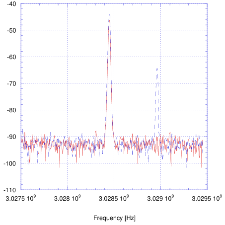
Figure 21: Power trasfer between the symmetric and the antisymmetric mode with in–phase piezo excitation (solid) and 180 degress out–of–phase excitation (dashed)

The explicit calculation of the coupling coefficient $C_{21}^{m}$ for an arbitrary deformation of the resonator volume can be done only by numerical methods. Analytic calculations showed that for an ideal spherical hollow resonator, excited in the fundamental quadrupolar mechanical mode and in the TE₀₁₁ electromagnetic mode, ${C_{21}^{m}}=1.9$. More detailed calculations, made on a realistic model of the coupled spheres, including the central coupling cell and the e.m. input and output ports, were made by finite element methods.

${\mathcal{H}}_{2}(t)$ is given by:

$${\mathcal{H}}_{2}(t)=\int_{0}^{\infty}K(\tau)f_{m}(t-\tau)\,d\tau=\frac{1}{2\pi}\int_{-\infty}^{+\infty}\widetilde{K}(\omega){\widetilde{f}}_{m}(\omega)\exp(i\omega t)\,d\omega\,;$$

$$K(\tau)=0\;{\mathrm{for}}\;\tau\leq 0\,.$$ (20)

The density of the external forces driving the motion of the system, i.e. the tides generated by the passing gravitational wave, are given by

$$f_{i}(\mathbf{r},t)=-\rho(\mathbf{r})R_{0i0j}(t)x^{j}\,,$$ (21)

where $\rho$ is the wall density, and $R_{0i0j}(t)$ are the components of the Riemann tensor evaluated in the center of mass of the solid. The components of the Riemann tensor can be expressed in terms of the adimensional amplitude of the g.w. $R_{0i0j}(t)=-1/2\,\ddot{a}_{ij}(t)$.

For a ”+” polarized plane g.w travelling along the $z$ axis the force density, in the proper reference frame attached to a detector lying in the $xy$ plane, has the form:

$$\mathbf{f}(\mathbf{r},t)=\frac{1}{2}\rho(\mathbf{r})\ddot{a}(t)\left[-x,y,0\right]\,,$$ (22)

with a similar expression for the ”$\times$” polarization. The generalized force, acting on the $m$ mechanical mode, then has the form

$$f_{m}(t)=-\frac{1}{2}\,\ddot{a}(t)\int_{Vol}\left[(\xi_{m})_{x}\,x-(\xi_{m})_{y}\,y\right]\rho(\mathbf{r})\,dV\,.$$ (23)

${\widetilde{f}}_{m}(\omega)$ is then given by:

$${\widetilde{f}}_{m}(\omega)=\frac{1}{2}\,M\omega^{2}{\mathcal{L}}\,{\widetilde{a}}(\omega)\,$$ (24)

having defined the detector’s effective length (for this mechanical mode and wave polarization):

$${\mathcal{L}}=\frac{1}{M}\int_{Vol}\left[(\xi_{m})_{x}\,x-(\xi_{m})_{y}\,y\right]\rho(\mathbf{r})\,dV\,$$ (25)

The function $\widetilde{K}(\omega)$ is found to be:

$$\widetilde{K}(\omega)=\frac{C^{m}_{21}\omega_{2}^{2}A_{1}/(2M)}{\left[\omega_{2}^{2}-(\omega+\omega_{1})^{2}+i\,\frac{\omega_{2}}{{\mathcal{Q}}}(\omega+\omega_{1})\right]\left[\omega_{m}^{2}-\omega^{2}+i\,\frac{\omega\omega_{m}}{Q_{m}}\right]-\frac{(C^{m}_{21}A_{1}\omega_{2})^{2}}{4M}}\,\exp(i\,\omega_{1}t)\,$$ (26)

The second term in the denominator of Eq. 26 is due to the back–action of the electromagnetic fields on the cavity walls. Its effect is particularly important when $\omega_{2}-\omega_{1}\approx\omega_{m}$. In this case optimum signal transfer does not correspond to the maximum field amplitude $A_{1}$ that can be stored in the initially excited mode (that is limited by the critical field of the superconductor, $H_{c}\approx 0.2$ T for niobium). Instead, optimum signal transfer is obtained from a lower value that has to be optimized according to the prevailing experimental conditions and detector characteristics. The dependence of the signal on the energy stored in the initially excited mode will be further discussed in Section VII.2 where the expected sensitivity of the detector in various experimental conditions is analyzed.

The average energy stored in mode number 2 is $U_{2}=1/2|{\mathcal{H}}_{2}(t)|^{2}$ and the power extracted from a cavity port coupled to an external load with a coupling coefficient $\beta_{2}$ is $P_{2}=\beta_{2}\,(\omega_{2}/{\mathcal{Q}})\,U_{2}$.

If $a(t)=h\alpha(t)$ with $\alpha(t)$ periodic at angular frequency $\Omega$, the expression of the output power from mode $2$ is given by $P_{2}={\mathcal{R}}(\Omega)\,h^{2}$, with

$${\mathcal{R}}(\Omega)=\frac{1}{4}\,\frac{\beta_{2}\omega_{2}}{{\mathcal{Q}}}\,\Omega^{4}M^{2}{\mathcal{L}}^{2}|\widetilde{K}(\Omega)|^{2}\,.$$ (27)

VIII.2 Noise

To study how the thermal fluctuations of the walls contribute to the output signal, we will start again from Eqs. 17–18, taking now the external force $f_{m}(t)$ as a stochastic force with constant power spectrum $S_{fm}=4Mk_{B}T\omega_{m}/Q_{m}$ papoulis . The output noise power spectral density is given by:

$$S_{PP}(\omega)=\frac{\beta_{2}\omega_{2}}{{\mathcal{Q}}}\,|\widetilde{K}(\omega)|^{2}S_{ff}$$ (28)

The thermal fluctuations of the electromagnetic field itself can be calculated in an analogus way. Starting again from Eqs. 17–18, we consider an external, stochastic force coupled to the magnetic field ${\mathcal{H}}_{2}(t)$, with constant power spectrum $S_{fe}=4kT/(\omega_{2}{\mathcal{Q}})$. The output noise spectral density is given by:

$$S_{{\mathcal{H}}{\mathcal{H}}}=\frac{\beta_{2}\omega_{2}}{{\mathcal{Q}}}\,|\widetilde{\chi}(\omega)|^{2}S_{fe}$$ (29)

with $\widetilde{\chi}(\omega)$ given by:

$$\widetilde{\chi}(\omega)=\frac{\omega_{2}^{2}\left(\omega_{m}^{2}-\omega^{2}+i\,\frac{\omega\omega_{m}}{Q_{m}}\right)}{\left[\omega_{2}^{2}-(\omega+\omega_{1})^{2}+i\,\frac{\omega_{2}}{{\mathcal{Q}}}(\omega+\omega_{1})\right]\left[\omega_{m}^{2}-\omega^{2}+i\,\frac{\omega\omega_{m}}{Q_{m}}\right]-\frac{(C^{m}_{21}A_{1}\omega_{2})^{2}}{4M}}\,.$$ (30)

We note that in the limit of vanishing coupling, $C^{m}_{21}\approx 0$, the contribution to the output noise of the walls vanishes, while the contribution of the electromagnetic field fluctuations tends to be like a simple harmonic oscillator of frequency $\omega_{2}$ and quality factor ${\mathcal{Q}}$.

Other noise sources must also be taken into account. To operate our device we have to feed microwave power into mode $1$, using an external rf source locked on mode $1$, at frequency $\omega_{1}$. The master oscillator phase noise is filtered through the resonator linewidth; the power spectral density has the following frequency dependence slater :

$$S_{MO}(\omega)=\frac{4\beta_{1}P_{i}/(\omega_{1}{\mathcal{Q}})}{\left(\frac{1}{{\mathcal{Q}}}\right)^{2}+\left(\frac{\omega+\omega_{1}}{\omega_{1}}-\frac{\omega_{1}}{\omega+\omega_{1}}\right)^{2}}$$ (31)

where $P_{i}$ is the power input level and $\beta_{1}$ is the coupling coefficient of mode $1$ to the output load. From the above equation we can estimate the microwave power noise spectral density at the detection frequency $\omega=\omega_{2}-\omega_{1}$:

$$S_{MO}(\omega_{2}-\omega_{1})\approx\beta_{1}\frac{P_{i}}{\omega_{1}{\mathcal{Q}}}\left(\frac{\omega_{2}}{\omega_{2}-\omega_{1}}\right)^{2}$$ (32)

This figure can be improved if the receiver discriminates the spatial field distribution of the e.m. field at frequency $\omega_{2}$, i.e. if it is sensitive only to the power excited in mode number $2$, rejecting all contributions coming from mode number $1$. In this way mode $1$ is decoupled from the output load and $\beta_{1}=0$. The experimental set–up, based on the use of two magic–tees which accomplishes this issue, is discussed in detail in rsi . Of course, the mode discrimination cannot be ideal, and some power leaking from mode $1$ to the detector’s output will be present. Nevertheless our previous work has demonstrated that with careful tuning of the detection electronics we can obtain $\beta_{1}\leq 10^{-14}$ rsi .

The input Johnson noise of the first amplifier in the detection electronics has to be added to the previous contributions to establish the overall noise spectral density. It can be described by the frequency independent spectral density papoulis :

$$S_{JJ}=k_{B}T(10^{(N/10)}-1)\equiv k_{B}T_{eq}$$ (33)

where $N$ is the noise figure of the amplifier (in dB) and $T$ the operating temperature. The equivalent temperature (or noise temperature) $T_{eq}$, is equal to the temperature (in Kelvin) of a 50 ohm termination at the input of an ideal noiseless amplifier with the same gain and generating the same output noise power.

Other noise sources (e.g. the seismic noise) are not considered in this paper.

We shall characterize the noise in our detector by a frequency dependent spectral density $S_{h}(\omega)$, with dimension Hz^-1 defined as

$$S_{h}(\omega)=\frac{S_{n}(\omega)}{{\mathcal{R}}(\omega)}$$ (34)

where $S_{n}=S_{PP}+S_{{\mathcal{H}}{\mathcal{H}}}+S_{MO}+S_{JJ}$, is the detector noise spectral density.

VIII.3 Sensitivity

Let us focus our attention on the system based on two spherical niobium cavities working at $\omega_{1}\approx\omega_{2}\approx 2$ GHz with a maximum stored energy in the initially excited symmetric mode of $U_{1}\approx 10$ J per cell (corresponding to a maximum surface magnetic field $H_{max}=0.1$ T, half the critical field of niobium). This is a small–scale system with an effective length of 0.1 m and a typical weight of 5 kg. The lowest quadrupolar mechanical mode is at $\omega_{m}\approx 4$ kHz. In the following, we shall consider an equivalent temperature of the detection electronics $T_{eq}=1$ K.

A possible design of the detector uses both the mechanical resonance of the structure, and the e.m. resonance. Due to the tuning system, the detection frequency can be made equal to the mechanical mode frequency $\omega_{m}\approx\omega_{2}-\omega_{1}$. The expected sensitivity of the detector for $\omega_{2}-\omega_{1}=\omega_{m}=4$ kHz is shown in figure 22, for a mechanical quality factor $Q_{m}=10^{3}$ (solid line) and $Q_{m}=10^{6}$ (dashed line). Note that, in the two cases, the optimum sensitivity is obtained with different values of stored energy. In both cases the stored energy has been optimized for maximum detector bandwidth. When the mechanical quality factor is higher ($Q_{m}=10^{6}$) the stored energy has to be maintained much under the maximum allowed value.

When $\omega_{2}-\omega_{1}=\omega_{m}$, the detector sensitivity is limited by the walls thermal motion. In this case, a lower $T_{eq}$ would increase the detection bandwidth.

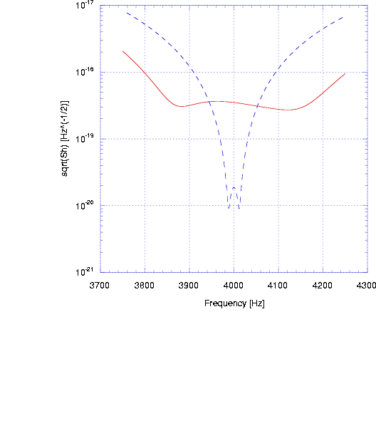
Figure 22: Calculated system sensitivity ($\omega_{m}\approx\omega_{2}-\omega_{1}\approx 4$ kHz, ${\mathcal{Q}}=10^{10}$, $T=1.8$ K, $T_{eq}=1$ K, and a) $Q_{m}=10^{3}$, stored energy $U\approx 10$ J per cavity (solid line); b) $Q_{m}=10^{6}$, stored energy $U\approx 0.1$ J per cavity (dashed line))

Since our detector is based on a double resonant system (the mechanical resonator and the electromagnetic resonator) it can be operated also for frequencies $\omega_{2}-\omega_{1}\neq\omega_{m}$. At frequencies $\omega_{2}-\omega_{1}\leq 1$ kHz the master oscillator phase noise will, in general, completely spoil the system sensitivity, while at frequencies $\omega_{2}-\omega_{1}\geq 10$ kHz the noise coming from the detection electronics will dominate. The expected sensitivity of the small–scale detector for $\omega_{2}-\omega_{1}=10$ kHz is shown in figure 23.

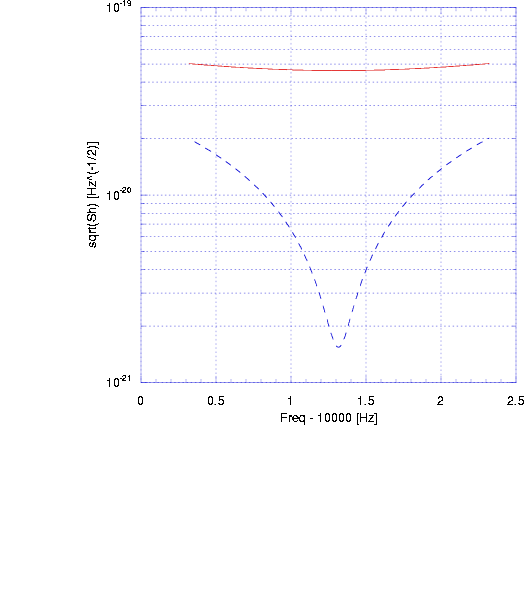
Figure 23: Calculated system sensitivity ($\omega_{m}\approx 4$ kHz, $\omega_{2}-\omega_{1}\approx 10$ kHz, ${\mathcal{Q}}=10^{10}$, $T=1.8$ K, $T_{eq}=1$ K, stored energy $U\approx 10$ J per cavity and a) $Q_{m}=10^{3}$ (solid line); b) $Q_{m}=10^{6}$ (dashed line))

In order to increase the expected sensitivity a large–scale system has to be developed. A possible design could be based on two spherical cavities working at $\omega_{1}\approx\omega_{2}\approx 500$ MHz, with $\omega_{m}\approx 1$ kHz. This system could have a maximum stored energy of $U_{1}\approx 1200$ J per cell, an effective length of 0.4 m and a typical weight of 2300 kg. With a reasonable choice of system parameters one could obtain the sensitivity shown in figure 24, for the double-resonance case ($\omega_{2}-\omega_{1}=\omega_{m}$). As in the previous (small–scale) case the energy store in the initially excite mode has been optimized for maximum bandwidth, and it has to be much less then the maximum allowed. Also in this case lowering $T_{eq}$ corresponds to an increase of the detection bandwidth.

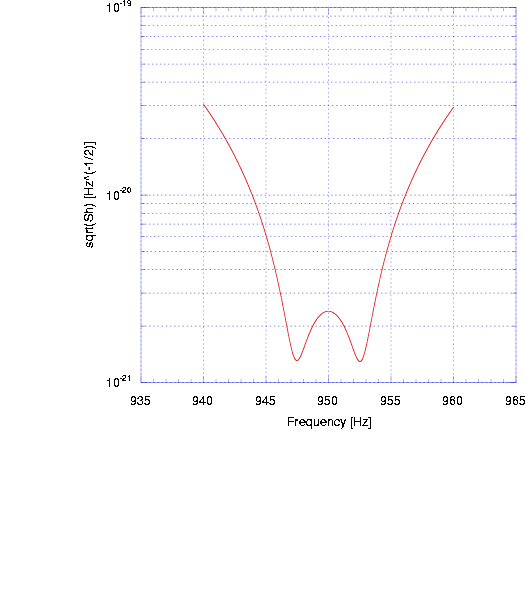
Figure 24: Calculated system sensitivity ($\omega_{m}\approx\omega_{2}-\omega_{1}\approx 1$ kHz, ${\mathcal{Q}}=10^{10}$, $Q_{m}=10^{6}$, $T=1.8$ K, $T_{eq}=1$ K, stored energy $U\approx 1$ J per cavity)

Obviously the large–scale system could also be used at higher frequencies; in this case a good sensitivity can be achieved in a narrow detection bandwidth (see Fig. 25).

It is worth noting that the narrow detection bandwidth is not an unavoidable drawback of the system. Actually its value is determined by the coupling coefficient of the antisymmetric mode at the $\Delta$ port of the output magic–tee, and can be adjusted changing this coupling. This corresponds to changing (lowering) the quality factor of the antisymmetric mode, leaving the quality factor of the symmetric mode unaffected. Of course an increased bandwidth corresponds to a lower sensitivity, since the latter is proportional to the antisymmetric mode quality factor. The possibility to increase the detection bandwidth is also interesting for other possible applications of this detection technique which is based on the parametric frequency conversion between two electromagnetic modes in a cavity (for example, in connection with recently proposed detectors based on the dual resonator concept dual1 ; dual2 ; dual3 ).

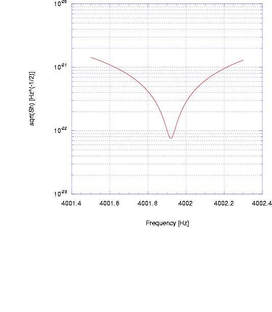
Figure 25: Calculated system sensitivity ($\omega_{m}\approx 1$ kHz, $\omega_{2}-\omega_{1}\approx 4$ kHz, ${\mathcal{Q}}=10^{10}$, $Q_{m}=10^{6}$, $T=1.8$ K, $T_{eq}=1$ K, stored energy $U\approx 1200$ J per cavity)

IX Data Analysis

Several aspects of MAGO data analysis need to be investigated.

The data-analysis for both single and multiple MAGOs will be akin of those used for acoustic detectors Finn , in view of the narrowband MAGO response.

Data analysis strategies for MAGOs operating above $f\sim 4\cdot 10^{3}$ Hz will be strictly non parametric, in view of the present lack of GW source/signal models in this frequency range.

Optimum MAGO tuning schedules for detecting unknown (sub)millisecond pulsars ms_PSR , ms_PSR1 will be obviously a most relevant issue to be investigated.

A ”xylophone” of MAGOs tuned in the range between $10^{3}$ Hz and $10^{4}$ Hz might be able to both detect and estimate the chirp-mass Finn1 of galactic light BH-MACHO binaries MACHO , which would produce a distinct signature in the xylophone output WG . The expected (optimistic) event-rate might be non negligible Finn .

Once MAGO prototypes will be up and running, a primary task will be to investigate the experimental noise PSD and transfer function, by comparison to their theoretical counterparts.

X Future Developments

The sensitivity of the device currently under test, consisting of a couple of nearly spherical niobium cells, 2 mm thick, whose total mass is approximately 4.5 kg, might be improved in several ways. Among these the most promising are:

• an increase of the mechanical quality factor of the structure;

• an increase of the electromagnetic quality factor of the superconducting cavities;

• a lower noise temperature of the detection electronics;

• the increase of the size (and mass) of the detector;

• the use of several detectors in an array or in a xylophone.

All these items are discussed in the following.

X.1 Increasing the mechanical quality factor

Although the $S/N$ ratio does depend on several parameters, we can state that if the noise power spectral density is limited by thermal noise, the minimum $S_{h}$ is proportional to the square root of the mechanical quality factor, $(Q_{m})^{1/2}$.

The mechanical quality factor depends both on the intrinsic mechanical energy dissipated in the material of the resonator and on the energy dissipated through the coupling to the external environment. The intrinsic quality factor of niobium at low temperature and few kHz is $Q_{m}\sim 10^{8}$. Since our detector is immersed in a bath of subcooled superfluid helium, improvements in $Q_{m}$ can be expected thanks to carefully designed liquid helium bath and suspension system.

The limit imposed by mechanical dissipation in the superfluid helium bath is $Q_{m}\sim 10^{6}$ for the present small–scale detector (see sec. VI.2).

This figure can be further improved for a larger detector ($M\gtrsim 10^{4}$ kg). In this case, the expected liquid–helium–limited mechanical quality factor should be $Q_{m}\sim 10^{7}$ (see sec. VI.2).

We remark that the above limits are essentially due to the will of using a well established refrigeration scheme for the superconducting cavity. In principle different schemes could be developed which do not make use of a bath of coolant in contact with the cavity (e.g. pulse tube refrigerators). Obviously this requires a consistent R&D effort which is not, for the time being, in the line of our proposal which is entirely based on already existing technologies.

X.2 Increasing the electrical quality factor

The gain in sensitivity due to the electrical quality factor, ${\mathcal{Q}}$, is less trivial to discuss. First of all a distinction should be made between the electromagnetic quality factor of the symmetric (pump) mode and of the antisymmetric (detection) mode. The quality factor of the pump mode, ${\mathcal{Q}}_{1}$, strongly affects the carrier (oscillator) phase noise and the energy stored in the cavity for a given input power. The quality factor of the detection mode, ${\mathcal{Q}}_{2}$, affects the shot noise power spectral density and the detection bandwidth.

For the sake of simplicity in our proposal these two quality factor were taken as equal: ${\mathcal{Q}}_{1}={\mathcal{Q}}_{2}={\mathcal{Q}}$. This is certainly a reasonable assumption as far as the intrinsic quality factor of the niobium spheres: ${\mathcal{Q}}_{0}=G/R_{s}$ is considered. In fact ${\mathcal{Q}}_{0}$ depends only on the geometrical shape of the resonator, on the electromagnetic resonant mode and on the surface quality. The overall (loaded) quality factor of a resonator, though, is given by ${\mathcal{Q}}={\mathcal{Q}}_{0}/(1+\beta)$, where $\beta$ is the coupling coefficient to the external load.

As a consequence, it is in general convenient to keep the quality factor of the pump mode ${\mathcal{Q}}_{1}$ as high as possible, in order to have the minimum power dissipation for a given energy stored in the detector (or the maximum stored energy for a given level of power dissipation) and the minimum carrier phase noise at the detection frequency. This requirement is fulfilled when $\beta_{1}\sim 1$ (critical coupling).

On the other hand, the value of the detection mode quality factor, ${\mathcal{Q}}_{2}$, is a parameter that has to be set to the optimum value (which depends on the specific experimental situation) by tuning the output coupling coefficient $\beta_{2}$. To be more specific, since shot noise and amplifier back–action noise are roughly proportional to $({\mathcal{Q}}_{2})^{-1/2}$, when either of these is the dominant noise contribution an higher ${\mathcal{Q}}_{2}$ gives better sensitivity (and, in general, a small detection bandwidth). On the contrary, when sensitivity is limited by other noise sources (e.g. thermal noise) it is convenient to lower ${\mathcal{Q}}_{2}$ (increasing $\beta_{2}$) to open the bandwidth.

Improvements in the intrinsic quality factor, ${\mathcal{Q}}_{0}$, can be expected thanks to specific Nb surface treatments that give a lower $R_{s}$. Quality factor values ${\mathcal{Q}}_{0}\gtrsim 10^{11}$ have already been measured on several prototypes of elliptical accelerating cavities ($R_{s}\sim 1$ nOhm) both bulk niobium safa , and sputtered niobium on copper sergio . Since those cavities were run on the TM₀₁₀ accelerating mode, we can expect ${\mathcal{Q}}_{0}\sim 10^{12}$ (on the TE₀₁₁ mode) with a comparable surface quality, due to the increased geometrical factor.

X.3 Increasing the performance of the detection electronics

A further headway can be foreseen using a low noise amplifier. The noise temperature of a cryogenic, commercially available, high–frequency amplifier (GaAs or InP HEMT device) is $T_{eq}=2$ K. Bearing in mind that we want to amplify an e.m. field at a frequency around $\omega/(2\pi)\sim 2$ GHz (much greater than the detection (g.w.) frequency $\Omega_{gw}=\omega_{2}-\omega_{1}$) one can easily see that the minimum (quantum limited) noise temperature of an amplifier is $T_{eq}=\hbar\omega/k_{B}\sim 0.1$ K.

This apparently high noise temperature though is not a drawback, since the parametric transducer operates the up–frequency conversion from low energy quanta $\hbar\Omega_{gw}\rightarrow\hbar\omega$ with no added noise. In this process the gain (in energy) is $\omega/\Omega_{gw}\sim 10^{6}$ (louisell2, , sec. 7.9–7.11).

In other words, the noise temperature seen at the input of the parametric up–converter is $T_{eq}\sim 0.1\times\Omega_{gw}/\omega\sim 10^{-7}$ K.

X.4 Increasing the size of the detector

Starting from the experience gathered with the existing small–scale prototype, a plausible detector (inner radius of the spherical cell $a=0.2$ m, thickness $w=5$ mm) could be designed and built.

Such detector might have the following parameters: overall mass $M\sim 44$ kg (approx. a ten–fold increase with respect to the present small–scale prototype), characteristic length $\mathcal{L}\sim 1$ m, working rf frequencies $\omega/(2\pi)\sim 1$ GHz, stored energy $U\sim 210$ J, detection frequency range $2$ kHz $\lesssim\Omega_{gw}/(2\pi)\lesssim 10$ kHz.

Being the detector tunable in frequency, we shall divide its use into two different working ranges: a Near Mechanical Resonance range (hereafter NMR) and an Off Mechanical Resonance range (OMR). NMR operation can only be used next to both quadrupolar mechanical resonances of the spherical shell (at frequencies $f_{1}\sim 2$ kHz and $f_{2}\sim 8$ kHz). The two ranges require quite different parameter sets and lead to optimized use of the detector, depending on the sources under investigation.

Fig. 26 and fig. 27 show system sensitivity calculated with $Q_{m}=10^{6}$ (limited by mechanical dissipation in liquid helium), ${\mathcal{Q}}_{0}=8.5\times 10^{11}$ and a nearly quantum limited electronics $T_{eq}=0.05$ K, in NMR and OMR mode. All other detector parameters are optimized for NMR and OMR operation. As expected, the use of $T_{eq}=0.05$ K for the noise temperature of the amplifier does not bring a dramatic increase in the peak performance of the system, whereas the bandwidth is strongly enhanced.

We remind that the bandwidth of the detector can be adjusted also by means of the electromagnetic coupling ($\beta_{2}$) as discussed in the previous section. Adjusting the electromagnetic coupling is of paramount importance because it allows trading maximum sensitivity versus bandwidth and is particularly useful when the maximum sensitivity is limited by thermal noise (NMR operation).

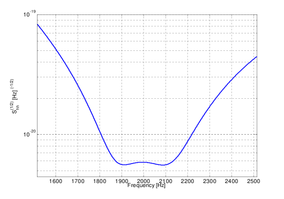
Figure 26: Near mechanical resonance PSD of one MAGO. Minimum $(S_{h})^{1/2}\sim 6\times 10^{-21}$ (Hz)^-1/2, bandwidth $\Delta f\sim 350$ Hz. Mechanical quality factor $Q_{m}=10^{6}$ (limited by losses in liquid helium), electrical intrinsic quality factor ${\mathcal{Q}}_{0}=8.5\times 10^{11}$ ($R_{s}=1$ nohm), amplifier equivalent temperature $T_{eq}=0.05$ K (quantum limit).

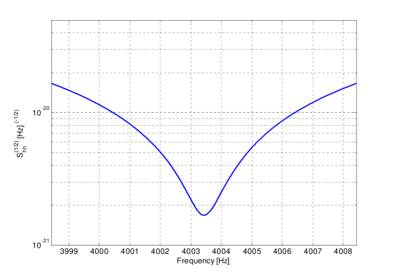
Figure 27: Off mechanical resonance PSD of one MAGO. Minimum $(S_{h})^{1/2}\sim 1.6\times 10^{-21}$ (Hz)^-1/2, bandwidth $\Delta f\sim 1$ Hz. Other parameters as in fig. 26.

X.5 Increasing the number of the detectors

A possibly nicer extension for the detector discussed in the previous section is given by multi–detector operation to achieve low false–alarm probabilities in coincidence operation. Furthermore, since MAGO can be designed to work at any chosen frequency in the range $10^{3}$–$10^{4}$ Hz with the same sensitivity, a ”xylophone” of MAGOs might be able to both detect and estimate the chirp mass of galactic light BH–MACHO binaries, which would produce a distinct signature in the xylophone output.

The expected (optimistic) event–rate might be not negligible (see section III.3).

Several authors have already pointed out the usefulness of array detectors, both for source localization and for improving the overall signal information (multimode transducer) frasca94 ; frasca96 ; frasca97 .

The SNR of $N$ optimally oriented detectors, sharing the same sensitivity band is approx. $N$ times the SNR of the single detector frasca94 . A set of 10 MAGOs would therefore have a peak $(S_{h})^{1/2}\sim 10^{-22}$ (Hz)^-1/2.

In building a MAGO coincidence network, several features of the small single detector add to the many known benefits of arrays:

• The expected cost and requirements confer a non negligible freedom in choosing the installation sites and financing;

• There is a greater freedom in the choice of the material;

• Short thermal cycle allow faster development phase and more flexible management of the instrument;

• High frequency operation is preferable from an instrumental point of view because many problems like vibration isolation, transducer optimization and amplifier matching are easier to solve;

• MAGO size makes it possible to more easily achieve optimal orientation among distant detectors. It makes also possible to host a local array in a reasonably limited area. This feature is particularly important in view of the detection of a stochastic background of GWs (see sec. III.5).

• Thanks to the frequency and bandwidth tuning ability, one could have a nearly complete overlap of the sensitivity, allowing narrow-band/high-sensitivity detection mode (OMR operation) not be a strong limitation. This feature might play a role in the detection of GW signals from binary mergers (see sec. III.1).

• High frequency signal sensitivity is apt to constructing high resolution images (see fig. 28).

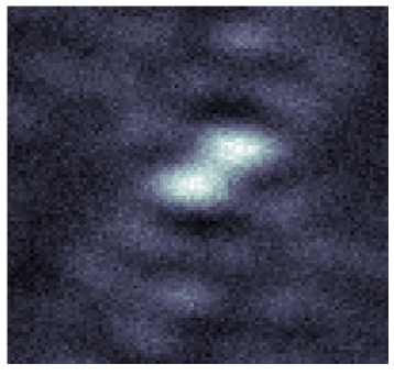
Figure 28: Reconstructed image (simulated) from a network of 10 MAGO detectors, with $SNR=0.5$ for the single detector. The angular distance between the two sources is $\Delta\theta=\Delta\phi=0.1\,{}^{\circ}$ and the shown portion of the sky is $1\,{}^{\circ}$ square.

References

-
(1)
http://www.roma1.infn.it/rog/
http://www.lnl.infn.it/ auriga/welcome.html
http://gravity.phys.lsu.edu/
http://www.gravity.pd.uwa.edu.au/. -
(2)
http://www.virgo.infn.it/
http://www.ligo.caltech.edu/
http://www.geo600.uni-hannover.de/
http://tamago.mtk.nao.ac.jp/tama.html
http://lisa.jpl.nasa.gov/. - (3) F. Pegoraro, L.A. Radicati, Ph. Bernard, and E. Picasso. Physics Letters, 68A(2):165–168, 1978.
- (4) F. Pegoraro, E. Picasso, and L.A. Radicati. Journal of Physics A, 11(10):1949–1962, 1978.
- (5) Ph. Bernard, G. Gemme, R. Parodi, and E. Picasso. Review of Scientific Instruments, 72(5):2428–2437, 2001. arXiv:gr-qc/0103006.
- (6) R. Ballantini, Ph. Bernard, E. Chiaveri, A. Chincarini, R. Losito, G. Gemme, R. Parodi, and E. Picasso. Classical and Quantum Gravity, 20(5):3505–3522, 2003.
- (7) A.J. Farmer and E.S. Phinney. astro-ph/0304393.
- (8) M.G. Haehnelt. Mon. Not. Roy. Astron. Soc., 269:199, 1994.
- (9) F.D. Ryan. Phys. Rev. D, 52:5707, 1995.
- (10) http://lisa.jpl.nasa.gov; http://sci.esa.int/home/lisa/.
- (11) V. Kalogera et al. Astrophys. J. Lett., 550, 2001.
- (12) A. Burrows and J. Hayes. Phys. Rev. Lett., 76:352, 1996.
- (13) B.J. Owen et al. Phys. Rev. D, 58:084020, 1998.
- (14) B. Allen and J.D. Romano. Phys. Rev. D, 59:102001, 1999.
- (15) http://vega.ess.sci.osaka-u.ac.jp/gwdaw/files/0401.pdf.
- (16) http://gravity.phys.lsu.edu/.
- (17) http://www.auriga.lnl.infn.it/.
- (18) http://www.roma1.infn.it/rog/explorer/explorer.
- (19) http://www.lnf.infn.it/esperimenti/rog/nautilus.
- (20) http://www.gravity.pd.uwa.edu.au.
- (21) L.S. Finn and S. Mukherjee. Phys. Rev. D, 63:062004, 2001.
- (22) S. M. Merkowitz and W. W. Johnson. Physical Review D, 51:2546, 1995.
- (23) http://www.minigrail.nl.
- (24) P. Astone et al. Nucl. Phys. Proc. Suppl., 70:461, 1999.
- (25) O.D. Aguiar et al. Class. Quantum Grav., 19:1949, 2002.
- (26) Ph. Bernard, A. Chincarini, G. Gemme, R. Parodi, and E. Picasso. In Proceedings of the Xth Workshop on Rf Superconductivity, Tsukuba, Japan, 2001. http://conference.kek.jp/SRF2001/pdf/PZ001.pdf.
- (27) B. Schutz. The case for broadband high frequency detectors. In Gravitational waves advanced detectors workshop (GWADW), Aspen, (CO), 2003.
- (28) K.D. Kokkotas and N. Andersson. Oscillation and instabilities of relativistic stars. In Recent developments in general relativity, Milan, Italy, 2002. Springer–Verlag. Proc. of the XIV Conference of general relativity and gravitational physics, Genoa, 2000.
- (29) K.D. Kokkotas. High frequency gravitational waves sources. Proc. of the Amaldi 5 International Conference on Gravitational Waves, Tirrenia, 2003.
- (30) J.A. Lobo. What can we learn about gw physics with an elastic spherical antenna? Physical Review D, 52:591, 1995.
- (31) P. Astone et al. Noise behaviour of the Explorer gravitational wave antenna during transition to the superfluid phase. Cryogenics, 32(7):668, 1992.
- (32) Ph. Bernard, G. Gemme, R. Parodi, and E. Picasso. Coupled microwave cavities for the detection of small harmonic displacements. Technical Report INFN/TC–98/17, INFN, 1998.
- (33) C.E. Reece, P.J. Reiner, and A.C. Melissinos. Observation of cm harmonic displacement using a 10 superconducting parametric converter. Physics Letters, 104A(6,7):341, 1984.
- (34) C.E. Reece, P.J. Reiner, and A.C. Melissinos. Parametric converters for detection of small harmonic displacements. Nuclear Instruments and Methods, A245:299–315, 1986.
- (35) J.C. Slater. Microwave Electronics. D. Van Nostrand Company, Inc., New York, 1950.
- (36) P.R. Saulson. Thermal noise in mechanical experiments. Physical Review D, 42(8):2437–2445, 1990.
- (37) A. Papoulis. Probability, Random Variables and Stochastic Processes. McGraw–Hill, New York, 1965.
- (38) M. Cerdonio et al. Wideband dual spere detector of gravitational waves. Physical Review Letters, 87:031101, 2001.
- (39) L. Conti et al. A wideband and sensitive gw detector for khz frequencies: The dual sphere. Classical and Quantum Gravity, 19:2013–2019, 2002.
- (40) M. Bonaldi et al. Selective readout and back-action reduction for wideband acoustic gravitational wave detectors. 2003. arXiv:gr-qc/0302012.
- (41) L.S. Finn. Gravitational radiation sources and signatures. arXiv:gr-qc/9903107, 1999.
- (42) J. Cordes and D.F. Chernoff. Astrophys J., 482:971, 1997.
- (43) L. Burderi et al. astro-ph/0109088, 2001.
- (44) L.S. Finn. Phys. Rev. D, 53:2878, 1996.
- (45) T. Nakamura et al. Astrophys . Lett., 487, 1997.
- (46) R.P. Croce et al. 2003.
- (47) W.H. Louisell. Coupled Mode and Parametric Electronics. John Wiley and Sons, New York, 1965.
- (48) H. Safa, Proc. X Workshop on RF Superconductivity, Tsukuba (Japan), 2001, paper MA008.
- (49) S. Calatroni, Proc. IX Workshop on RF Superconductivity, Santa Fe (NM, USA), 1999, paper MOA002.
- (50) W.H. Louisell, Radiation and Noise in Quantum Electronics, McGraw–Hill, New York, 1964.
- (51) S. Frasca, M.A. Papa, Proc. I Amaldi Conference on Gravitational Waves, Frascati, 1994.
- (52) S. Frasca, Proc. International Conference on Gravitational Waves, Cascina, 1996.
- (53) S. Frasca, Proc. II Amaldi Conference on Gravitational Waves, CERN, 1997.
- (54) S.A. Hughes, Phys. Rev. D66, 102001, 2002.
- (55) R. Oechslin et al., ArXiv:astro-ph/0401083, 2004.
- (56) V. Kalogera, ArXiv:astro-ph/9911532, 1999.
- (57) T. Damour et al., Phys.Rev. D67, 064028 2003.
- (58) E.S. Phinney, Astrophys. J. Lett., 380, L17, 1991.
- (59) C. Kim, V. Kalogera and D.R. Lorimer, Astrophys. J., 584(1), 985, 2003.
- (60) M. Burgay et al., Nature, 426, 531, dec. 2003.
- (61) V. Kalogera et al., Astrophys. J., 556, 340, 2001.
- (62) E.E. Flanagan, S. Hughes, Phys. Rev. D57, 4535, 1998.
- (63) P. Astone et al., Class. Quant. Grav. 19 5449, 2002.
- (64) L.S. Finn, Phys. Rev. D53, 2878, 1996.
- (65) T. Nakamura et al., Astrophys. J. 487, L139, 1997.
- (66) M.S. Turner et al., arXiv:astro-ph/9601168, 1996.
- (67) L.S. Finn, arXiv:gr-qc/9609027, 1996.
- (68) J.C.N. de Araujo et al., Class. Quantum Grav., 21, S521, 2004.
- (69) T. Nakamura et al., Astrophys. J., 487, L139, 1997.
- (70) G.B. Cook, S.L. Shapiro, S.A. Teukolsky, Astrophys. J., 423, L117, 1994.
- (71) D. Madsen, Phys. Rev. Lett., 81, 3311, 1998.
- (72) E.S. Phinney amd S.R. Kulkarni, Ann. Rev. Astron. Astroph., 32, 591, 1994
- (73) N. Andersson, Astrophys. J., 708, 1998.
- (74) Ph. Arras et al., arXiv:astro-ph/0202345, 2003.
- (75) R.T. Edwards et al., Astroph. J., 560, 365, 2001.
- (76) J. Han et al., arXiv:astro-ph/0310640v1, 2003.
- (77) N. Christensen, Phys. Rev. D46, 5250 ,1992.
- (78) J.A. Lobo and A. Montero, arXiv:gr-qc/0206062, 2002.
- (79) N. Cornish, arXiv:gr-qc/0106058, 2001.
- (80) P. Astone et al., Astron. & Astropjys., 351, 811, 1999.
- (81) M. Cerdonio, E. Coccia, A. Ortolam, S. Vitale, Phys. Rev, D55, 1741, 1997.
- (82) B. Allen and J.D. Romano, Phys. Rev. D59, 102001, 1999.
- (83) P. Astone, J.A. Lobo and B.F. Schutz, Class. Quantum Grav., 11, 2093, 1994.
- (84) J.T. Whelan et al., arXiv:gr-qc/0308045, 2002.
- (85) B. Abbott et al., arXiv:gr-qc/0312088, 2003.
- (86) P.D. Edmonds and J. Lamb, Proc. Phys. Soc. LXXI (I), 1957.
- (87) S.J. Putterman, Superfluid Hydrodynamics, North Holland, Amsterdam, 1974.
- (88) D.C. Mattis and J. Bardeen, Phys. Rev. 111 (2), 412–417, 1958.
- (89) M.W. Zemansky, Heat And Thermodynamics , McGraw–Hill, New York, 1968.
- (90) G. Claudet et al., Proc. ICEC 12, Southampton, 1988, pag. 497.
- (91) P. Berglund et al., Physica B, Volumes 284-288, Part 2, July 2000, Pages 2012–2013.
- (92) G. Claudet et al., Proc. ICEC 12, Southampton, 1988, pag. 511.