Quantum evolution of the Universe from $\tau=0$ in the constrained quasi-Heisenberg picture

Abstract

The Heisenberg picture of the minisuperspace model is considered. The suggested quantization scheme interprets all the observables including the Universe scale factor as the (quasi)Heisenberg operators. The operators arise as a result of the re-quantization of the Heisenberg operators that is required to obtain the hermitian theory. It is shown that the DeWitt constraint $H=0$ on the physical states of the Universe does not prevent a time-evolution of the (quasi)Heisenberg operators and their mean values. Mean value of an observable, which is singular in a classical theory, is also singular in a quantum case. The (quasi)Heisenberg operator equations are solved in an analytical form in a first order on the interaction constant for the quadratic inflationary potential. Operator solutions are used to evaluate the observables mean values and dispersions. A late stage of the inflation is considered numerically in the framework of the Wigner-Weyl phase-space formalism. It is found that the dispersions of the observables do not vanish at the inflation end.

1 Introduction

A focus of the article is the construction of the quantization scheme in which the observables (including Universe scale factor) are the time dependent operators. This allows to evaluate their mean values and dispersions.

A variety of the quantization schemes for the minisuperspace model can be roughly divided in two classes: imposing the constraint ”before quantization” [1] and ”after quantization”[2]. In the former the constraints are used to exclude the ”nonphysical” degrees of freedom. This allows then to construct the Hamiltonian acting in the reduced ”physical” phase space.

The last schemes prefer imposing the constraint ”after quantization”. This leads to the Wheeler-DeWitt equation on quantum states of the Universe [2, 3]. Our scheme can be considered among the last class because we use the Wheeler-DeWitt equation. However we supplement this equation with the system of the quasi-Heisenberg operators acting in the space of the solutions of this equation. Quantization rules for these operators are defined consistently with the choice of the hyperplane used for normalization of the solutions of the Wheeler-deWitt equation in the Klein-Gordon style.

In the simplest case of an isotropic and uniform Universe filled with a scalar field, the minisuperspace equation contains only two variables: the scale factor of Universe and the amplitude of the scalar field. There is no an explicit ”time” in the corresponding Wheeler-deWitt equation, whereas we are interested namely in the Universe evolution in time. This leads to various discussions about ”time disappearance” and interpretation of the wave function of Universe [4]. Possible solutions like to introduce time along the quasi-classical trajectories, or subdivide Universe into classical and quantum parts were offered [6]. Such point of view can not be satisfactory. Ideally, time does exist independently regardless of whether we consider Universe quantum or classically. That forces to consider the quantum evolution of Universe without any need in foreign ingredients [7, 10, 11, 12]. Let us remind that this situation is analogous to that in string theory, where the constraint $H=0$ also exists. Nevertheless this constraint does not prevent an evolution of the Heisenberg operators $\hat{X}(\sigma,\tau)$ along $\tau$ [13].

In fact the constraint $H=0$ (in a theory of the constrained systems $H$ is usually refereed as the super-Hamiltonian) tells nothing about whether the mean values of the Heisenberg operators evolve with time or not. This is defined by the normalization of the wave function. We can outline an issue in the following way. Let there is the wave function $\psi(a,x)$ dependent on two variables and obeying $\hat{H}\psi(a,x)=0$.

For evolution of some Heisenberg operator $\hat{H}$ we have

$$<A(\tau)>=<\psi|e^{i\hat{H}\tau}\hat{A}e^{-i\hat{H}\tau}|\psi>.$$ (1)

At first sight it seems that there is no evolution. However this is not the case. Really $e^{-i\hat{H}\tau}|\psi>=|\psi>$, but we cannot write $<\psi|e^{i\hat{H}\tau}=<\psi|$. The point is that the wave function can not be normalized in the ordinary way $\int\psi^{*}(a,x)\psi(a,x)dxda=1$ due to the constraint. In fact the function is unbounded along one of the variables. For instance, let this is $a$ variable. So if $H$ contains differential operator like $\frac{\partial^{2}}{\partial a^{2}}$, one cannot move $\frac{\partial^{2}}{\partial a^{2}}$ to the left by the habitual operation $<\psi|\frac{\partial^{2}}{\partial a^{2}}=<\frac{\partial^{2}}{\partial a^{2}}\psi|$ through the integration by parts. As a result, the assumption that $<\psi|\hat{H}=<\hat{H}\psi|=0$ is wrong.

Unfortunately this is an oversimplified picture. Reality was found to be more complicated. In the next section we show that the normalization of the wave function in the Klein-Gordon style permits evolution of the mean values of the Heisenberg operators. However, additional efforts are needed to obtain a genuine hermitian theory.

2 Quantization of a particle-clock

The problem of the quantum cosmology has many common features with those of the relativistic particle [1, 13, 14, 15]. The action for the relativistic particle can be defined as:

$$S=-m\int\sqrt{-\dot{x}_{\mu}^{2}}d\tau.$$ (2)

The equivalent form leading to Eq. (2) by means of variation of the lapse function $e(\tau)$ is

$$S=\frac{1}{2}\int(e^{-1}\dot{x}_{\mu}^{2}-e\,m^{2})d\tau,$$ (3)

where $(-,+,+,+)$ signature is used. One more equivalent form resulting in (3) due to varying $p_{\mu}$ looks as

$$S=\int\bigl{\{}p_{\mu}\dot{x}^{\mu}-e\left(\frac{p_{\mu}^{2}+m^{2}}{2}\right)\bigr{\}}d\tau.$$ (4)

Using the re-parameterization invariance [13, 14] we can choose the lapse function as $e=1/m$. One can see from the last equation that the Hamiltonian is equal to $H=\frac{p_{\mu}^{2}+m^{2}}{2m}$ and vanishes on the constraint surface $H=0$ after varying on $e$. The quantization procedure is based on the assumptions:

$$[\hat{p}^{\mu},\hat{x}^{\nu}]=-ig^{\mu\nu},~{}~{}~{}~{}\hat{p}^{\mu}=\{\hat{\varepsilon},\hat{\bm{p}}\}\equiv\{i\frac{\partial}{\partial t},-i\bm{\nabla}\}.$$

Then the constraint becomes the Klein-Gordon equation. The commutators of the position and four-momentum operators with the Hamiltonian result in the Heisenberg equation of motion:

$$\frac{d\hat{x}^{\mu}}{d\tau}=i[\hat{H},\hat{x}^{\mu}]=\frac{\hat{p}^{\mu}}{m},~{}~{}~{}~{}~{}~{}\frac{d\hat{p}^{\mu}}{d\tau}=0.$$ (5)

Evident solution of the motion equation is

$$\hat{x}^{\mu}(\tau)=x^{\mu}+\frac{p^{\mu}(0)}{m}\,\tau,~{}~{}~{}\hat{p}^{\mu}(\tau)=\hat{p}^{\mu}(0),$$

where $\hat{x}^{\mu}(0)=x^{\mu}\equiv\{t,\bm{r}\}$ and $\hat{p}^{\mu}(0)=\hat{p}^{\mu}$. Because before quantization we do not use any gauge fixing providing the time-dependent second class constraint [14], $\hat{t}(\tau)$ can be treated as an operator. We shall refer to $\hat{t}(\tau)$ as ”physical time” and to $\tau$ as ”proper time”. Whereas the physical time is operator, the proper time is some parameter ”always running forward” like time in the Newtonian physics.

One can check that the wave function satisfying the Klein-Gordon equation cannot be normalized through the integration over $d^{4}x$ [6]. However, it can be normalized through the time-like component of the conserved four-current:

$$<\psi|\psi>=-i\int\{\psi(\bm{r},t)\partial_{t}\psi^{*}(\bm{r},t)-(\partial_{t}\psi(\bm{r},t))\psi^{*}(\bm{r},t)\}d^{3}\bm{r}.$$

Normalized wave packets have the form:

$$\psi(x)=\int\frac{a(\bm{k})e^{-i\varepsilon(\bm{k})t+i\bm{k}\bm{r}}}{\sqrt{2\varepsilon(\bm{k})(2\pi)^{3}}}d^{3}\bm{k};~{}~{}~{}\int\mid a(\bm{k})\mid^{2}d^{3}\bm{k}=1,$$

where $\varepsilon^{2}(\bm{k})=\bm{k}^{2}+m^{2}$. To avoid an appearance of the states with the negative norm we have to choose only positive frequency solutions. For this wave packet the integration $\int\psi^{*}(x)\psi(x)d^{4}x$ does not converge. Hence the wave function is unbounded along the $t$-variable.

Let us define the mean value of some Heisenberg operator $\hat{A}(\tau)$ for the case of a free relativistic particle as

$$<\hat{A}(\tau)>=\frac{-i}{2}\int\biggl{(}\psi^{*}(\bm{r},t)\hat{A}(\bm{r},t,\hat{\varepsilon},\hat{\bm{p}},\tau)\partial_{t}\psi(\bm{r},t)$$

$$~{}~{}~{}~{}~{}~{}~{}~{}~{}~{}~{}~{}~{}~{}~{}~{}~{}~{}~{}~{}~{}~{}~{}~{}~{}~{}-(\partial_{t}\psi^{*}(\bm{r},t))\hat{A}(\bm{r},t,\hat{\varepsilon},\hat{\bm{p}},\tau)\psi(\bm{r},t)\biggr{)}d^{3}\bm{r}\biggr{|}_{t=0}+h.c.,$$ (6)

where $"h.c."$ means the hermitian conjugate value.

The definition (6) has the following properties:

1) It is consistent with the normalization of the wave function if we choose $\hat{A}$ to be equal to the unit operator.

2) It looks like as an expression for the mean value of the Heisenberg operator in the nonrelativistic picture when the operator acts on the wave function taken at the initial moment of time (note, that after integration over $d^{3}\bm{r}$ we have to set $t=0$).

3) It has a natural property $\frac{<\hat{A}(\tau)>}{d\tau}=<\frac{\hat{A}(\tau)}{d\tau}>$.

4) It gives zero for the physical time, when the proper time is equal to zero.

Figure 1: (a) Observer describing a particle motion by own clock, (b) Observer describing a particle motion by ”particle clock”.

Let us emphasize the difference between our quantization scheme for the relativistic particle and e.g. the quantization schemes (in the ADM style with the some gauge fixing or in the Foldy-Wouthauthen representation of the Klein-Gordon equation) where the time is not an operator. Let consider some observer with an ”exact” clock tracking a particle motion. The observer can measure, for instance, the particle coordinate and describe it by the operator $\hat{\bm{r}}(t)$ to take into account the quantum fluctuations. There remain only technical problems like to find the Hamiltonian translating $\hat{\bm{r}}(t)=e^{i\hat{H}t}\hat{\bm{r}}(0)e^{-i\hat{H}t}$ etc. Let consider another situation, namely the observer has no a clock but there is an exact ”clock” on the particle (e.g., this is the ”radioactive” particle emitting photons every equal time pieces in a reference system connected with the particle). The observer having no own clock is forced to measure time by the particle clock. The measured time is the fluctuating value described by the operator $\hat{t}(\tau)=\frac{\hat{\varepsilon}}{m}\tau$, because the particle energy $\varepsilon$ is the fluctuating quantity for the wave packet. Thus our quantization scheme describes namely the particle clock (i.e. the particle supplied with the clock) rather than the ”mute” particle.

After averaging, the Heisenberg equations of motion result in

$$<\hat{t}(\tau)>=<\hat{\varepsilon}>\frac{\tau}{m},~{}~{}<\hat{\bm{r}}(\tau)>=<{\bm{r}}>+<\hat{\bm{p}}>\frac{\tau}{m}.$$ (7)

One can see that the physical time is proportional to the proper time. It is interesting to calculate the dispersion of the physical time for the Gaussian wave packet $a(\bm{k})\sim e^{-\alpha\bm{k}^{2}}$ with the $\frac{1}{\alpha}>>m^{2}$. An evaluation of the mean values of $\hat{\varepsilon}=i\frac{\partial}{\partial t}$ and its square gives:

$$<\hat{\varepsilon}>=\frac{\int_{0}^{\infty}\varepsilon(k)e^{-\alpha k^{2}}k^{2}dk}{\int_{0}^{\infty}e^{-\alpha k^{2}}k^{2}dk}\approx\frac{2}{\sqrt{\pi\alpha}},~{}~{}<\hat{\varepsilon}^{2}>=\frac{\int_{0}^{\infty}\varepsilon^{2}(k)e^{-\alpha k^{2}}k^{2}dk}{\int_{0}^{\infty}e^{-\alpha k^{2}}k^{2}dk}\approx\frac{3}{2\alpha},$$

that results in

$$\frac{\sqrt{<\hat{t}^{2}>-<\hat{t}>^{2}}}{<\hat{t}>}=\frac{\sqrt{<\hat{\varepsilon}^{2}>-<\hat{\varepsilon}>^{2}}}{<\hat{\varepsilon}>}=\sqrt{\frac{3\pi}{8}-1}.$$

Thus, the ”particle-clock” is a bad clock when the particle is localized in the spatial region less than the Compton wave length. Let us imagine what occurs when the particle possessing the electric charge is placed in the electric field. Let there is a cloud of the particles with some initial dispersion of the energy placed in the electric field. The particles begin to accelerate in the electric field and thereby they receive the energies much larger than their initial energies. As a result the relative energy dispersion becomes negligible. Similar picture holds for the quantum case so that the relative accuracy of the ”particle-clock” increases.

Let us remind that in fact we have used here the covariant proper time formalism, which goes down to Fock [16] and Kramers [17]. This formalism is widely used for derivation of the Bargman-Michel-Telegdi equations for the particle spin motion in the external fields [18]. In this formalism we have to normalize the wave function through the Klein-Gordon scalar product instead of normalization through the integration over $d^{4}x$ (on the other side this permits the time-evolution despite of $\hat{H}\psi=0$). Absence of hermicity leads to the complex mean value of some observables. Although we are try to avoid a complexity by adding ”$h.c.$” quantity in Eq. (6) the negative dispersion appears when we evaluate, for instance, $<\hat{t}^{4}(\tau)>$ etc. Thus we have seen that the imposing constraint to the state vectors is not sufficient to obtain a ”good” theory in the framework of the covariant proper time formalism. In next section we shall propose solution for this problem.

3 Quantum cosmology

Let us start from the Einstein action of a gravity and the action for an one-component real scalar field:

$$S=\frac{1}{16\pi G}\int d^{4}x\sqrt{-g}R+\int d^{4}x\sqrt{-}g[\frac{1}{2}(\partial_{\mu}\phi)^{2}-V(\phi)],$$ (8)

where $R$ is the scalar curvature and $V$ is the matter potential which includes a possible cosmological constant effectively. We restrict our consideration to the homogeneous and isotropic metric:

$$ds^{2}=N^{2}(\tau)d\tau^{2}-a^{2}(\tau)d\sigma^{2}.$$ (9)

Here the lapse function $N$ represents the general time coordinate transformation freedom. For the restricted metric the total action becomes

$$S=\int N(\tau)\biggl{\{}\frac{3}{8\pi G}a\left({\mathcal{K}}-\frac{\dot{a}^{2}}{N^{2}(\tau)}\right)+\frac{1}{2}a^{3}\frac{\dot{\phi}^{2}}{N^{2}(\tau)}-a^{3}V(\phi)\biggr{\}}d\tau,$$

where $\mathcal{K}$ is the signature of the spatial curvature. This action can be obtained from the following expression by varying on $p_{a}$ and $p_{\phi}$

$$S=\int\biggl{\{}p_{\phi}\dot{\phi}+p_{a}\dot{a}-N(\tau)\biggl{(}-\frac{3a{\mathcal{K}}}{8\pi G}-\frac{8\pi G\,p_{a}^{2}}{12a}+\frac{p_{\phi}^{2}}{2a^{3}}+a^{3}V(\phi)\biggr{)}\biggr{\}}d\tau.$$

Varying on $N$ gives the primary constraint

$$H=-\frac{3a{\mathcal{K}}}{8\pi G}-\frac{8\pi G\,p_{a}^{2}}{12a}+\frac{p_{\phi}^{2}}{2a^{3}}+a^{3}V(\phi)=0.$$ (10)

After quantization $[\hat{a},\hat{p}_{a}]=-i$, $[\hat{\phi},\hat{p}_{\phi}]=i$ this constraint turns into the DeWitt equation $\hat{H}\psi(a,\phi)=0.$ Looking at the constraint equation a desire may appear to modernize or remove it [19]. Apparently this implies (both on classical and on quantum levels) existence of some preferred system of reference. Although there are some logically consistent theories implying preferred system of reference, for instance, the Logunov relativistic theory of gravity [20] giving an adequate description of the Universe expansion [21], we shall keep to the General Relativity here and retain the constraint.

Let us first consider the flat Universe (${\mathcal{K}}=0$) with $V(\phi)=0$ (corresponding Hamiltonian is $\hat{H}_{0}$).

Procedure, which is invariant under a general coordinate transformation consists in postulating the quantum Hamiltonian [24]

$$\hat{H}_{0}=\frac{1}{2}g^{-\frac{1}{4}}\hat{p}_{\mu}g^{\frac{1}{2}}\hat{g}^{\mu\nu}\hat{p}_{\nu}g^{-\frac{1}{4}},$$ (11)

where $\hat{p}_{\mu}=-ig^{-\frac{1}{4}}\,\frac{\partial}{\partial x^{\mu}}\,g^{\frac{1}{4}}=-i\left(\frac{\partial}{\partial x^{\mu}}+\frac{1}{4}(\frac{\partial\ln g}{\partial x^{\mu}})\right)$. For our choice of variables $x^{\mu}=\{a,\phi\}$, $p_{\mu}=\{-p_{a},p_{\phi}\}$ metric has the form (in the units $4\pi G/3=1$) $g^{\mu\nu}\ =\left(\begin{array}[]{cc}-\frac{1}{a}&\;0\\ &\\ \,\,0&\;\frac{1}{a^{3}}\end{array}\right),$ so that $g=a^{4}$, $\hat{p}_{a}=i\left(\frac{\partial}{\partial a}+\frac{1}{a}\right)$ and the Hamiltonian is

$$\hat{H}_{0}=-\frac{1}{4}\left(\hat{p}_{a}^{2}\frac{1}{a}+\frac{1}{a}\hat{p}_{a}^{2}\right)+\frac{\hat{p}_{\phi}^{2}}{2a^{3}}=\frac{1}{2a^{2}}\frac{\partial}{\partial a}a\frac{\partial}{\partial a}-\frac{1}{2a^{3}}\frac{\partial^{2}}{\partial\phi^{2}}.$$ (12)

Explicit expression for the wave function satisfying $\hat{H}_{0}\psi=0$ is

$$\psi_{k}(a,\phi)=a^{\pm i|k|}e^{ik\phi}.$$

Exactly as in the case of the Klein-Gordon equation we should choose only the positive frequency solutions [6]. Such wave function corresponds to the definite choice of the boundary condition for the minisuperspace: the wave function is formed by the modes bounded on $k$ and only ingoing in a singularity.

Thus the wave packet

$$\psi(a,\phi)=\int c(k)\frac{a^{-i|k|}}{\sqrt{4\pi|k|}}e^{ik\phi}dk$$ (13)

will be normalized by

$$ia\int\left(\frac{\partial\psi}{\partial a}\psi^{*}-\frac{\partial\psi^{*}}{\partial a}\psi\right)d\phi=\int c^{*}(k)c(k)dk=1.$$ (14)

The proper time evolution of the operators

$$\frac{d\hat{A}(\tau)}{d\tau}=i[\hat{H},\hat{A}]$$

results in

$$~{}{\hat{p}}_{\phi}^{\bm{\cdot}}(\tau)=0,~{}~{}{\hat{p}}_{\phi}(\tau)=const,~{}~{}(\hat{a}^{3}(\tau))^{\bm{\cdot}}=\frac{3}{2}\left(\hat{p}_{a}a+a\hat{p}_{a}\right),~{}~{}\frac{3}{2}(\hat{p}_{a}a+a\hat{p}_{a})^{\bm{\cdot}}=-9\hat{H}_{0}.$$ (15)

Set of equations for the Heisenberg operators and the constraint equation for the states would be considered as a tool to evaluate the mean values of observables. The obstacle is that the operators are hermite relatively an integration over $\sqrt{g}d^{n}x$, while due to constraint the states can not be normalized in such a way and are normalized in the Klein-Gordon style.

Our recept consists in enforcing the constraints on the equation of motion for the Heisenberg operators at $\tau=0$. First let us remind the Dirac quantization procedure [25] and return to the classical picture for this goal. According to Dirac, besides the primary constraint $\Phi_{1}=-\frac{p_{a}^{2}}{a}+\frac{p_{\phi}^{2}}{a^{3}}$ (see (10)), we have to set some additional gauge fixing (secondary) constraint, which can be chosen in our case as $\Phi_{2}=a-const$, because the hyperplane $a=const$ is chosen earlier for the normalization of the wave function in the Klein-Gordon style. In contrast to the usual formalism [1, 14, 26, 27]) we impose constraints $\Phi_{1}=0$ and $\Phi_{2}=0$, which have to be satisfied only at hyperplane $\tau=0$. Besides the ordinary Poisson brackets

$$\{A,B\}=\frac{\partial A}{\partial p_{\mu}}\frac{\partial B}{\partial x^{\mu}}-\frac{\partial A}{\partial x^{\mu}}\frac{\partial B}{\partial p_{\mu}},$$ (16)

the Dirac brackets are introduced

$$\{A,B\}_{D}=\{A,B\}-\{A,\Phi_{i}\}(C^{-1})_{ij}\{\Phi_{j},B\},$$ (17)

where $C$ is the nonsingular matrix with the elements $C_{ij}=\{\Phi_{i},\Phi_{j}\}$ and $C^{-1}$ is the inverse matrix. Quantization consists in the substitution of the commutators in the Dirac brackets and the replacement of the variables by the operators:

$$[\hat{\bm{\eta}},\hat{\bm{\eta}}^{\prime}]=-i\{\bm{\eta},\bm{\eta}^{\prime}\}_{D}\biggr{|}_{\bm{\eta}\rightarrow\hat{\bm{\eta}}}.$$ (18)

Here $\bm{\eta}$ implies the set of the canonical variables $p_{\mu},x^{\nu}$.

The Heisenberg equations of motion have to satisfy the constraints at initial moment $\tau=0$ and the operators obey the commutation relations obtained from the Dirac quantization procedure. Direct evaluation gives

$$[{\hat{p}}_{a}(0),{\hat{a}}(0)]=0,~{}~{}~{}{[\hat{p}_{\phi}(0),\hat{a}(0)]=0},$$

$${[{\hat{p}}_{\phi}(0),{\hat{\phi}}(0)]=-i},~{}{[{\hat{p}}_{a}(0),~{}\hat{\phi}(0)]=-i\frac{{\hat{p}}_{\phi}(0)}{{\hat{p}}_{a}(0){\hat{a}}^{2}(0)}}.$$ (19)

We have to solve the equations (15) with the given initial commutation relations. This changes the canonical commutation relations between the Heisenberg operators at $\tau\neq 0$. Therefore we shall call theirs as the quasi-Heisenberg operators. In fact we appeal to the structure of the classical theory and re-quantize the equations of motion.

One can see that the commutation relations (19) can be satisfied through

$$\hat{a}(0)=const=a,~{}~{}\hat{p}_{\phi}(0)=\hat{p}_{\phi},~{}~{}\hat{p}_{a}(0)=|\hat{p}_{\phi}|/a,~{}~{}\hat{\phi}(0)=\phi,$$ (20)

where $\hat{p}_{\phi}=-i\frac{\partial}{\partial\phi}$. Variable $a$ is $c$-number now because it commutes with all operators [27]. Solutions of the equations (15) are

$$\hat{p}_{\phi}(\tau)=\hat{p}_{\phi},~{}~{}~{}~{}\hat{\phi}(\tau)=\phi+\frac{\hat{p}_{\phi}}{3|\hat{p}_{\phi}|}\ln(a^{3}+3|\hat{p}_{\phi}|\tau)-\frac{\hat{p}_{\phi}}{|\hat{p}_{\phi}|}\ln\,a,$$

$$\hat{p}_{a}(\tau)=\frac{|\hat{p}_{\phi}|}{(a^{3}+3|\hat{p}_{\phi}|\tau)^{1/3}},~{}~{}~{}~{}\hat{a}^{3}(\tau)=a^{3}+3|\hat{p}_{\phi}|\tau,$$

We imply that these quasi-Heisenberg operators act in the Hilbert space with the Klein-Gordon scalar product.

Mean value of some operator $\hat{A}(\tau)$ can be defined as [29]:

$$<\hat{A}(\tau)>=ia\int\biggl{(}\psi^{*}(a,\phi)\hat{A}(\tau,\phi,\hat{p}_{\phi},a)\frac{\partial\psi(a,\phi)}{\partial a}~{}~{}~{}~{}~{}$$

$$-\frac{\partial\psi^{*}(a,\phi)}{\partial a}\hat{A}(\tau,\phi,\hat{p}_{\phi},a)\psi(a,\phi)\biggr{)}d\phi\biggr{|}_{a\rightarrow 0}.~{}~{}$$ (22)

However we shall use another definition:

$$<\hat{A}(\tau)>=i\,a\int\biggl{(}\psi^{*}(a,\phi)D^{\frac{1}{4}}\hat{A}(\tau)D^{-\frac{1}{4}}\frac{\partial}{\partial a}\psi(a,\phi)~{}~{}$$

$$-\frac{\partial}{\partial a}\psi^{*}(a,\phi)D^{-\frac{1}{4}}\hat{A}(\tau)D^{\frac{1}{4}}\psi(a,\phi)\biggr{)}d\phi\biggr{|}_{a\rightarrow 0},~{}~{}$$ (23)

where operator $D=-\frac{\partial^{2}}{\partial\phi^{2}}+2\,a^{6}V(\phi)$ (since $a\rightarrow 0$ the $V$-term can be omitted in the expression for $D$). The mean value (23) is particular case of that suggested in Ref. [30], where an one-particle picture of the Klein-Gordon equation in the Foldy-Wouthausen representation is considered. The advantage of this normalization can been seen in the momentum representation of $\phi$ variable, where $\hat{p}_{\phi}=k$ and $\hat{\phi}=i\frac{\partial}{\partial k}$. Eq. (22) gives

$$<\hat{A}(\tau)>=\frac{1}{2}\int{a}^{i|k|}\sqrt{|k|}c^{*}(k)\hat{A}(\tau,\hat{\phi},k,a)a^{-i|k|}{{c(k)}\over{\sqrt{|k|}}}dk$$

$$+\frac{1}{2}\int{a}^{i|k|}{{c^{*}(k)}\over{\sqrt{|k|}}}\hat{A}(\tau,\hat{\phi},k,a)a^{-i|k|}\sqrt{|k|}c(k)dk\biggr{|}_{a\rightarrow 0},~{}~{}$$

while Eq. (23) leads to

$$<\hat{A}(\tau)>=\int{a}^{i|k|}c^{*}(k)\hat{A}(\tau,\hat{\phi},k,a){a}^{-i|k|}c(k)dk\biggr{|}_{a\rightarrow 0},$$ (24)

which is similar to the ordinary quantum mechanics and certainly posses hermicity.

Evaluation of the mean value over the wave packet gives

$$<a^{3}(\tau)>=3\tau\int|k||c(k)|^{2}dk.$$ (25)

If we assume that there is no external ”physical time” in Universe (proper time $\tau$ hardly can be considered as the measurable observable), then we must take some quantity, for instance, $<a^{3}(\tau)>$ as the ”physical time”.

Next interesting quantity is the mean value of the scalar field $<\hat{\phi}(\tau)>$:

$$<\hat{\phi}(\tau)>_{a}=\int{a}^{i|k|}c^{*}(k)\left(i\frac{\partial}{\partial k}+\frac{k}{3|k|}\ln\left(a^{3}+3|k|\tau\right)-\frac{k}{|k|}\ln a\right)a^{-i|k|}c(k)dk$$

$$=\int\left(c^{*}(k)i\frac{\partial}{\partial k}c(k)+\frac{k}{3|k|}\ln\left(a^{3}+3|k|\tau\right)|c(k)|^{2}\right)dk.$$ (26)

Brackets $<\dots>_{a}$ with the index $a$ in (26) mean that we do not set $a$ equal to zero yet (compare with Eq. (24)). A remarkable property of Eq. (26) is that the term $-\frac{k}{|k|}\ln a$ cancels the term arising from the differentiation: $a^{i|k|}i\frac{\partial}{\partial k}a^{-i|k|}=\frac{k}{|k|}\ln a$. Thus we may get to $a\rightarrow 0$ and obtain

$$<\hat{\phi}(\tau)>=\int\left(\frac{k}{3|k|}\ln(3|k|\tau)|c(k)|^{2}+c^{*}(k)i\frac{\partial}{\partial k}c(k)\right)dk.$$ (27)

Cancellation of the terms divergent under $a\rightarrow 0$ in the mean values of the quasi-Heisenberg operators is a general feature of the theory, and give us possibility to evaluate, for instance,

$$<\hat{\phi}^{2}(\tau)>=\int\biggl{(}\frac{1}{9}\ln^{2}(3|k|\tau)|c(k)|^{2}-c^{*}(k)\frac{\partial^{2}}{\partial k^{2}}c(k)\biggr{)}dk.$$ (28)

One should not confuse the divergence at $a\rightarrow 0$ arising under evaluation of the mean values with the singularity at $\tau\rightarrow 0$. The mean values of operators, which are singular at $\tau\rightarrow 0$ in classical theory remain singular also in the quantum case. The way to avoid a singularity is to guess, that Universe was burn not from a point but from a ”seed” of $a_{0}$-”size”. Then in the expression for mean value we have to assume $a\rightarrow a_{0}$ instead of $a\rightarrow 0$. This puts a question about underling theory giving size of the seed.

One more kind of the infinity can be found in Eqs. (27), (28). For $c(k)$, which does not tend to zero at small $k$ the mean values of $\phi(\tau)$ and $\phi^{2}(\tau)$ diverge. This is a manifestation of the well known infrared divergency of the scalar field minimally coupled with gravity. Thus not all possible $c(k)$ are suitable for the construction of the wave packets.

Let us consider Hamiltonian, containing the cosmological constant $V_{0}$:

$$\hat{H}=\hat{H}_{0}+a^{3}V_{0}.$$ (29)

Explicit solution for the wave function $H\psi=0$ has the form

$$\psi_{k}(a,\phi)=\left(\frac{18}{V_{0}}\right)^{\frac{i|k|}{6}}\Gamma(1-\frac{i|k|}{3})J_{-\frac{i|k|}{3}}(\frac{\sqrt{2V_{0}}}{3}a^{3})e^{ik\phi},$$ (30)

where $\Gamma(z)$ is the Gamma function and $J_{\mu}(z)$ is the Bessel function. The wave function (30) tends to $a^{-i|k|}e^{ik\phi}(1+O(a^{6}))$ asymptotically under $a\rightarrow 0$. If we assume that the operators of all physical quantities are local on the $a$ variable or can be approximated by the local ones, then for an evaluation of the mean values we may always build the wave packet from the functions $a^{-i|k|}e^{ik\phi}$. This supply ideology of the usual nonrelativistic Heisenberg picture which says that all dynamics is contained in the Heisenberg operators and only knowledge of the wave function is required. The argumentation holds for any potential $V(\phi)$, because it contributes into the Hamiltonian as a term multiplied by $a^{3}$.

Equations of motion obtained from the Hamiltonian (29) are

$$(\hat{a}^{3}(\tau))^{\bm{\cdot}}=\frac{3}{2}(\hat{p}_{a}a+a\hat{p}_{a});$$ (31)

$$\frac{3}{2}(\hat{p}_{a}a+a\hat{p}_{a})^{\bm{\cdot}}=9V_{0}a^{3}-9\hat{H}_{0};$$ (32)

$$9(V_{0}a^{3}-\hat{H}_{0})^{\bm{\cdot}}=18V_{0}\frac{3}{2}(\hat{p}_{a}a+a\hat{p}_{a}).$$ (33)

The additional term $a^{3}V_{0}$ does not change relations (19) required for the re-quantization procedure. Only expression for $\hat{p}_{a}(0)$ changes in (20): $\hat{p}_{a}(0)=\sqrt{\frac{\hat{p}_{\phi}^{2}}{a^{2}}+2V_{0}a^{4}}$.

Finally we arrive to

$$\hat{a}^{3}(\tau)=a^{3}+3|\hat{p}_{\phi}|\frac{\sinh(\tau\sqrt{18V_{0}})}{\sqrt{18V_{0}}}+a^{3}(\cosh(\tau\sqrt{18V_{0}})-1).$$ (34)

Evaluation of the mean values according to Eq. (23) leads to

$$<\hat{a}^{3}(\tau)>=\frac{\sinh(3\,\sqrt{2V_{0}}\,\tau)}{\sqrt{2V_{0}}}\int|k||c(k)|^{2}dk,$$

$$<\hat{a}^{6}(\tau)>=\frac{\left({\sinh(3\,\sqrt{2V_{0}}\,\tau)}\right)^{2}}{2\,V_{0}}\int k^{2}|c(k)|^{2}dk.$$

This shows, that the dispersion $\frac{\sqrt{<\hat{a}^{6}>-<\hat{a}^{3}>^{2}}}{<\hat{a}^{3}>}$ does not depend on $\tau$, exactly as in the case of the free relativistic particle. Thus in this model the evolution of Universe remains quantum during all time. This results from the absence of any scale length (but not from an ambiguity of the wave function normalization; see, for instance, Ref. [32]). Such a length appears if we take $V(\phi)=\frac{m^{2}\phi^{2}}{2}$. One may suggest that the expansion of Universe remains quantum until the moment, when the scaling factor approaches the Compton wave length $1/m$. When $<a(\tau)>$ becomes greater than $1/m$ the expansion can be described classically. To see this explicitly we have to find the quasi-Heisenberg solutions with the above potential.

4 Operator equations for the quadratic inflationary potential

As it has been discussed the quantization procedure is reduced to the quantization of the equations of motion i.e. considering them as the operator equations, which have to be solved with the initial conditions satisfying to the constraint at $\tau=0$. For the Hamiltonian

$$H=-\frac{p_{a}^{2}}{2a}+\frac{p_{\phi}^{2}}{2a^{3}}+a^{3}g\frac{\phi^{2}}{2}$$ (35)

we have the equations

$$\ddot{a}=-\frac{3}{2}a\dot{\phi}^{2}-\frac{\dot{a}^{2}}{2a}+\frac{3}{2}ag\phi^{2},$$

$$\ddot{\phi}=-3\frac{\dot{a}}{a}\dot{\phi}-g\phi$$ (36)

and the constraint

$$-{\dot{a}^{2}}{a}+{\dot{\phi}^{2}}{a^{3}}+a^{3}g\phi^{2}=0.$$ (37)

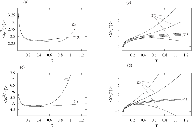
Figure 2: Mean values of the square of the scalar field and the logarithm of the Universe scale factor calculated in the zero (1) and first orders (2) on $g=1$, for the wave packet $c(k)=\frac{4}{\sqrt{3}}\left(\frac{2}{\pi}\right)^{1/4}k^{2}\,\exp(-k^{2})$ – Fig. (a), (b), and for the wave packet $c(k)=\left(\frac{2}{\pi}\right)^{1/4}\,\exp(-k^{2}-\frac{1}{k^{2}}+2)$ – Fig. (c), (d). Each of the triplets of the curves in Fig. (b), (d) corresponds to the $<\hat{\alpha}(\tau)>-\sqrt{D(\tau)}$ (lower), $<\hat{\alpha}(\tau)>$ (medial), $<\hat{\alpha}(\tau)>+\sqrt{D(\tau)}$ (upper), where $D=<\hat{\alpha}^{2}(\tau)>-<\hat{\alpha}(\tau)>^{2}$.

The point means the differentiation over $\tau$. After quantization Eqs. (36) lead to the equations for the quasi-Heisenberg operators, which have to be solved with the operator initial conditions

$$\hat{a}(0)\equiv a,~{}~{}~{}\hat{\phi}(0)\equiv\phi,~{}~{}~{}\hat{p}_{\phi}(0)\equiv-i\frac{\partial}{\partial\phi},~{}~{}~{}\dot{\hat{\phi}}(0)=\frac{\hat{p}_{\phi}(0)}{\hat{a}^{3}(0)}=\frac{1}{a^{3}}\left(-i\frac{\partial}{\partial\phi}\right),$$

$$\dot{\hat{a}}(0)=\hat{a}(0)\sqrt{\dot{\hat{\phi}}^{2}(0)+g{\hat{\phi}}^{2}(0)}=\sqrt{\frac{1}{a^{4}}\left(-i\frac{\partial}{\partial\phi}\right)^{2}+ga^{2}\phi^{2}}.$$ (38)

According to our ideology the operator constraint (37) is satisfied only at $\tau=0$. The ordinary problem of the operator ordering arises, because in the general case the quasi-Heisenberg operators are noncommutative. The problem becomes more transparent if we change the variable $\hat{\alpha}=\ln\hat{a}$:

$$\ddot{\hat{\alpha}}+\frac{3}{2}\dot{\hat{\alpha}}^{2}-\frac{3}{2}g\,\hat{\phi}^{2}+\frac{3}{2}{\dot{\hat{\phi}}}^{2}=0,$$

$${\ddot{\hat{\phi}}}+\frac{3}{2}\left(\dot{\hat{\alpha}}\dot{\hat{\phi}}+\dot{\hat{\phi}}\dot{\hat{\alpha}}\right)+g\hat{\phi}=0.$$ (39)

This system has to be solved with the initial conditions $\hat{\phi}(0)\equiv\phi$, $\hat{\alpha}(0)=lna$, $\hat{\dot{\phi}}(0)=\frac{1}{a^{3}}\left(-i\frac{\partial}{\partial\phi}\right)$, $\dot{\hat{\alpha}}(0)=\sqrt{g\phi^{2}+\frac{1}{a^{6}}\left(-i\frac{\partial}{\partial\phi}\right)^{2}}$. We have used the symmetric ordering in Eq. (39).

The operator equations under consideration can be solved within the framework of the perturbation theory in the first order on interaction constant. The solution in analytical form is given in Appendix. The calculations of the mean values based on (24) have been carried out with the two kinds of the wave packets: $c(k)=\frac{4}{\sqrt{3}}\left(\frac{2}{\pi}\right)^{1/4}k^{2}\,\exp(-k^{2})$ and $c(k)=e^{2}\left(\frac{2}{\pi}\right)^{1/4}\,\exp(-k^{2}-\frac{1}{k^{2}})$, which were normalized as $\int_{\infty}^{\infty}|c(k)|^{2}dk=1$. Because of the infrared divergency we must take only wave packets with vanishing $c(k)$ at $k\rightarrow 0$. The results of the calculations are shown in Figs. 2. The packets under consideration are symmetric thus the mean value of the scalar field vanishes. In the first order on $g$ we can consider only an early beginning of the inflation. At this stage the square of the the scalar field grows due to initial ”kinetic energy”. The logarithm of the scale factor grows linearly.

As it has been discussed in the previous section in the zero-order on $g$, the relative dispersion of $\hat{a}^{3}(\tau)$ does not depend on $\tau$ so that the dispersion of $\hat{\alpha}(\tau)=\ln\,\hat{a}(\tau)$ is constant. In the first order on $g$ we might expect that the dispersion of the scale factor should decrease and the quantum universe will approach to the classical one. However, we see an opposite picture: the dispersion of $\alpha$ grows with $\tau$. However, as it is suggested in Ref. [34] some mechanism of the classical world appearance has to exist.

5 Wigner-Weyl evolution of the minisuperspace

The analysis of the inflation at its late stages requires a numerical consideration of the operator equations that can be realized within the framework of the Weyl-Wigner phase-space formalism [29]. Let us remind that in this formalism every operator acting on $\varphi$ variable have the Weyl symbol: ${\mathcal{W}}[\hat{A}]=A(k,\phi)$. The simplest Weyl symbols reads: $\mathcal{W}[-i\frac{\partial}{\partial\phi}]=k$, ${\mathcal{W}[\phi]=\phi}$. Weyl symbol of the symmetrized product of operators has the form

$$W[\frac{1}{2}(\hat{A}\hat{B}+\hat{B}\hat{A})]=\cos\left(\frac{\hbar}{2}\frac{\partial}{\partial\phi_{1}}\frac{\partial}{\partial k_{2}}-\frac{\hbar}{2}\frac{\partial}{\partial\phi_{2}}\frac{\partial}{\partial k_{1}}\right)A(k_{1},\phi_{1})B(k_{2},\phi_{2})\biggr{|}_{k_{1}=k_{2}=k,\,\phi_{1}=\phi_{2}=\phi}\,,$$

where the Plank constant is restored only to point up to which order we will expand the cosine in the next. This has no direct physical meaning because the effects of the quantum mechanics are contained as in the Weyl symbols, so in the Wigner function, and the last one has no limit at $\hbar\rightarrow 0$ in the general case [29].

Let us consider the Weyl transformation of Eqs. (39) and expand the Weyl symmetrized product of operators up to second-order in $\hbar$. This results in:

$$\partial^{2}_{\tau}\alpha+\frac{3}{2}\biggl{(}(\partial_{\tau}\alpha)^{2}+\frac{\hbar^{2}}{4}(\partial_{k}\partial_{\phi}\partial_{\tau}\alpha)^{2}-\frac{\hbar^{2}}{4}(\partial^{2}_{\phi}\partial_{\tau}\alpha)(\partial^{2}_{k}\partial_{\tau}\alpha)\biggr{)}+\frac{3}{2}\biggl{(}(\partial_{\tau}\varphi)^{2}+\frac{\hbar^{2}}{4}(\partial_{k}\partial_{\phi}\partial_{\tau}\varphi)^{2}$$

$$-\frac{\hbar^{2}}{4}(\partial^{2}_{\phi}\partial_{\tau}\varphi)(\partial^{2}_{k}\partial_{\tau}\varphi)\biggr{)}-\frac{3}{2}g\biggl{(}\varphi^{2}+\frac{\hbar^{2}}{4}(\partial_{k}\partial_{\phi}\varphi)^{2}-\frac{\hbar^{2}}{4}(\partial^{2}_{\phi}\varphi)(\partial^{2}_{k}\varphi)\biggr{)}=0,$$

$$\partial^{2}_{\tau}\varphi+3\biggl{(}\partial_{\tau}\alpha\partial_{\tau}\varphi+\frac{\hbar^{2}}{4}(\partial_{k}\partial_{\phi}\partial_{\tau}\alpha)(\partial_{k}\partial_{\phi}\partial_{\tau}\varphi)-\frac{\hbar^{2}}{8}(\partial^{2}_{k}\partial_{\tau}\alpha)(\partial^{2}_{\phi}\partial_{\tau}\varphi)$$

$$~{}~{}~{}~{}~{}~{}~{}~{}~{}~{}~{}~{}~{}~{}~{}~{}~{}~{}~{}~{}~{}~{}~{}~{}~{}~{}~{}~{}~{}~{}~{}~{}~{}~{}~{}~{}~{}-\frac{\hbar^{2}}{8}(\partial^{2}_{\phi}\partial_{\tau}\alpha)(\partial^{2}_{k}\partial_{\tau}\varphi)\biggr{)}+g\varphi=0.$$ (40)

where $\alpha(k,\phi,\tau)$ and $\varphi(k,\phi,\tau)$ are the Weyl symbols of the operators $\hat{\alpha}(\tau)$ and $\hat{\phi}(\tau)$, respectively. These equations have to be solved with the initial conditions at $\tau=0$:

$$\alpha\left(k,\phi,0\right)=\ln\left(a\right),~{}~{}\partial_{\tau}\alpha\left(k,\phi,0\right)={\mathcal{W}}\left[\sqrt{-{\frac{{1}}{{a^{6}}}\frac{\partial^{2}}{\partial\phi^{2}}+g\phi^{2}}}\right],\hfill$$

$$\varphi\left(k,\tau,0\right)=\phi,~{}~{}~{}~{}\partial_{\tau}\varphi\left(k,\tau,0\right)=\frac{k}{{a^{3}}}.\hfill$$ (41)

Weyl symbol of the square root [33] can be expressed as

$${\mathcal{W}}\left[\sqrt{-{\frac{{1}}{{a^{6}}}\frac{\partial^{2}}{\partial\phi^{2}}+g\phi^{2}}}\right]=\frac{g^{1/4}}{\pi^{1/2}a^{3/2}}\int_{0}^{\infty}t^{-1/2}\exp\left(-\frac{g\,a^{6}\phi^{2}+k^{2}}{\sqrt{g}\,a^{3}}\tanh(t)\right)$$

$$\times\mbox{sech}(t)\left(\frac{g\,a^{6}\phi^{2}+k^{2}}{\sqrt{g}\,a^{3}}\mbox{sech}(t)^{2}+\tanh(t)\right)dt,$$ (42)

but since the mean values are calculated in the limit $a\rightarrow 0$, we can take simply $\partial_{\tau}\alpha\left(k,\phi,0\right)=\frac{|k|}{a^{3}}$ (this will not change the mean values).

State of the Universe in this approach is described by the Wigner function $\wp(k,\phi)$, which is constructed on the basis of definition (23). That gives:

$$\wp\left({k,\phi}\right)=ia\int{\left[{\left|{-\frac{{\partial^{2}}}{{\partial\phi^{2}}}}\right|^{-\frac{1}{4}}\psi^{*}\left({\phi+\frac{u}{2}}\right)}\right]\left[{\left|{-\frac{{\partial^{2}}}{{\partial\phi^{2}}}}\right|^{\frac{1}{4}}\frac{{\partial\psi\left({\phi-\frac{u}{2}}\right)}}{{\partial a}}}\right]e^{iku}du}-\hfill$$

$$ia\int{\left[{\left|{-\frac{{\partial^{2}}}{{\partial\phi^{2}}}}\right|^{\frac{1}{4}}\frac{{\partial\psi^{*}\left({\phi+\frac{u}{2}}\right)}}{{\partial a}}}\right]\left[{\left|{-\frac{{\partial^{2}}}{{\partial\phi^{2}}}}\right|^{-\frac{1}{4}}\psi\left({\phi-\frac{u}{2}}\right)}\right]e^{iku}du,}\hfill$$ (43)

or in the momentum representation of the wave function corresponding to Eq. (13):

$$\wp(k,\phi)=\frac{1}{\pi}\int c^{*}(2k-q)c(q)a^{-i|q|+i|2k-q|}e^{2i(q-k)\phi}dq.$$ (44)

As a result of $a\rightarrow 0$, both Weyl symbols and Wigner function diverge. In particular, when $a\rightarrow 0$ the Wigner function becomes more and more oscillating. However the divergences cancel each other in the expectation values constructed in the ordinary way. For instance, expectation values of $\alpha$ and its square are:

$$\left\langle\alpha(\tau)\right\rangle=\int{dkd\phi\,\alpha(k,\phi,\tau)\wp\left({k,\phi}\right)}|_{a\rightarrow 0}\,,$$

$$\left\langle\alpha^{2}(\tau)\right\rangle=\int dkd\phi\left(\alpha^{2}+\frac{\hbar^{2}}{4}(\partial_{k}\partial_{\phi}\alpha)^{2}-\frac{\hbar^{2}}{4}(\partial^{2}_{\phi}\alpha)(\partial^{2}_{k}\alpha)\right)\wp({k,\phi})\biggr{|}_{a\rightarrow 0}.$$

An example of the Wigner function for the wave package with $c\left(k\right)=\frac{4}{{\sqrt{3}}}\left({\frac{2}{\pi}}\right)^{\frac{1}{4}}k^{2}\exp\left({-k^{2}}\right)$ is shown in Fig. 3.

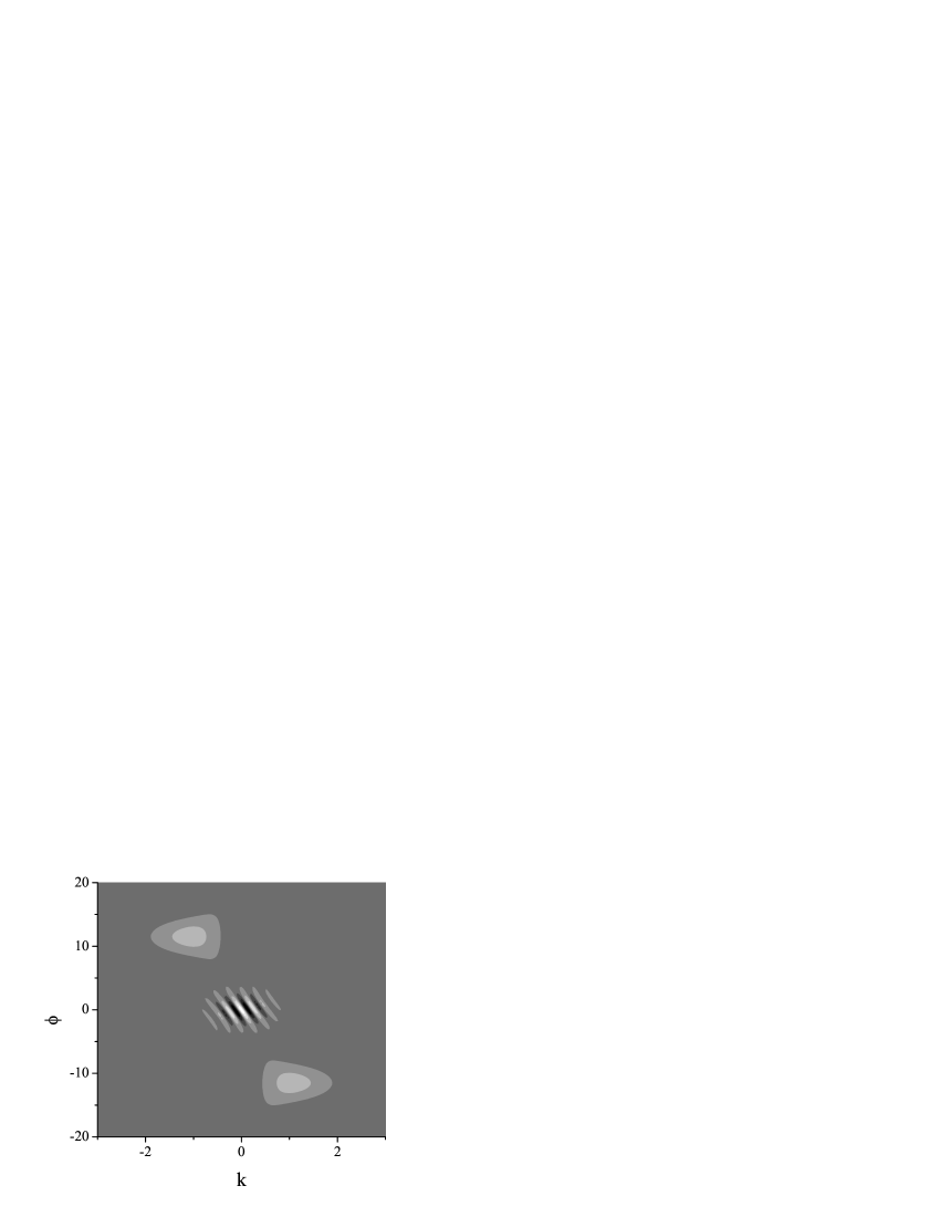
Figure 3: Contour-plot of the Wigner function of universe at $a=10^{-5}$.

As a result of numerical solution of Eqs. (40), we have obtained the evolution of the operators expectation values and their dispersions. Some results are shown in Figs. (4-6). We have considered three wave packages providing suppression of the infrared (and certainly ultraviolet) divergence. For our rather illustrative calculations, the ”cuts off” of the wave packets are chosen of order unity i.e. at the Plankian level. In principal, the ”cuts off” have to be consistent with the sub-Planskian physics eliminating divergences at fundamental level. In other words we describe Planskian physis here, but all sub-Planskian physics should be contained in the functions of $c(k)$.

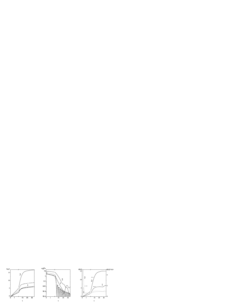
Figure 4: Evolution of $\left\langle\alpha\right\rangle,\,\left\langle{\varphi^{2}}\right\rangle$, dispersion $\sigma\left(\alpha\right)=\sqrt{\left\langle{\alpha^{2}}\right\rangle-\left\langle\alpha\right\rangle^{2}}$ (black curves) and relative dispersion $\sigma\left(\alpha\right)/\left\langle\alpha\right\rangle$ (gray curves) for $c\left(k\right)=\frac{4}{{\sqrt{3}}}\left({\frac{2}{\pi}}\right)^{\frac{1}{4}}k^{2}\exp\left({-k^{2}}\right)$. $\hbar=0$ (1), 1 (2). For comparison we give the classical evolution with the same initial conditions (initial $k$ is 0 (dashed) and $\sqrt{\left\langle{k^{2}}\right\rangle}$ (dotted), initial $\phi=$$\sqrt{\left\langle{\phi^{2}}\right\rangle}$). $a=10^{-4}$.

It is of interest to compare the evolution numerically obtained for the arbitrary coupling parameter $g$ with that obtained from the analytical operator evaluation in the first-order expansion on $g$ (see previous Section). We consider two different cases for Eqs. (40): i) $\hbar=0$ (quasi-classical evolution) and ii) $\hbar=1$ (quantum corrections; note, that in the previous sections we didn’t use any expansion on $\hbar$).

In addition to results of previous Section, we can see the deceleration of the initial exponential expansion of the universe and the transition to the post-inflationary scenario. In the quasi-classical case the evolution of expectations can be considered as a good approximation to the classical scenario (curves 1 and dashed (or dotted) curves, respectively). However, the inflaton oscillations are smeared in the quasi-classical case due to presence of the modes with different $k$. Choice of the more ”cold” wave package, i.e. the package with the suppressed high-frequency modes, enhances the inflation (Fig. 5). Some enhancement of inflation results also from the removing of the low-frequency components from the wave package (Fig. 6).

The quantum corrections (second-order in $\hbar$) essentially affect the evolution at the initial stage. As it was demonstrated in previous Section, there is the stage when the scalar field rolls away the minimum of potential due to kinetic energy of the wave package (some analog exists also in the classical case, see dotted curves in Fig. 4). As a result, the inflation intensifies. However, in any case the inflation comes to the end.

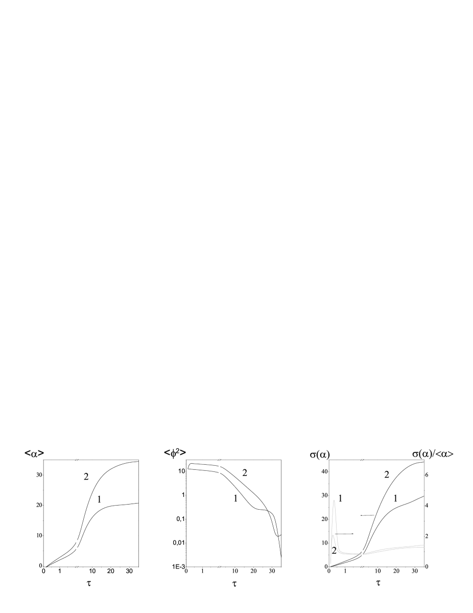
Figure 5: As in Fig. 4 but for $c\left(k\right)=\frac{20}{{\sqrt{3}}}\left({\frac{10}{\pi}}\right)^{\frac{1}{4}}k^{2}\exp\left({-5k^{2}}\right)$.

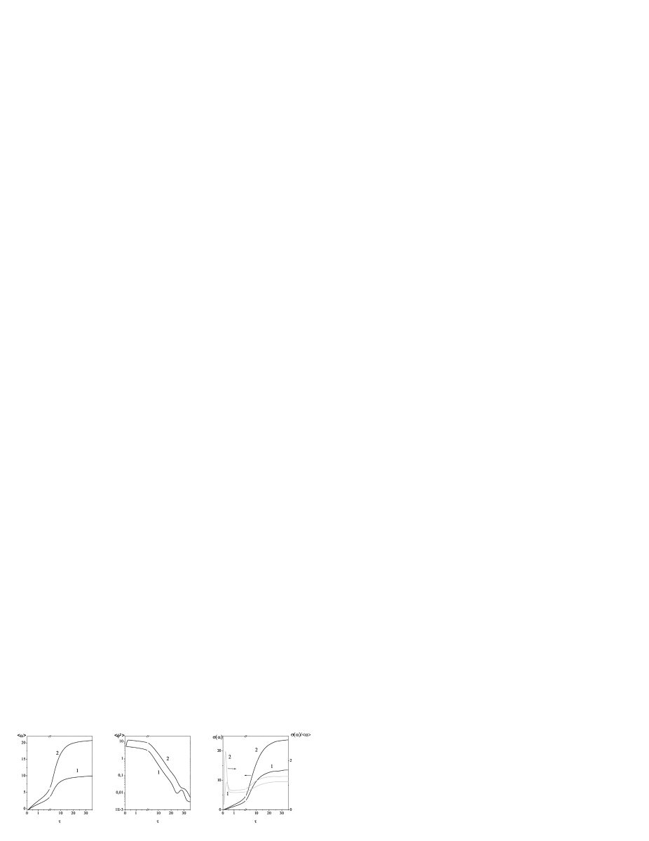
Figure 6: As in Fig. 4 but for $c\left(k\right)=e^{2}\left({\frac{2}{\pi}}\right)^{\frac{1}{4}}\exp\left({-k^{2}-1/k^{2}}\right)$.

It is important, that in all cases the relative dispersion reaches some maximum and then decreases. However, the relative dispersion does not vanish but approaches some asymptotical value, which does not differ essentially for the different wave packages. It is astonishing that the asymptotical relative dispersion is similar in quasi-classical and in quantum-corrected cases. This suggests that some mechanism of the classical world appearance is required. Such mechanism is absent in our simplest model. We surmise that this can be some decoherence produced by the additional degrees of freedom.

6 Conclusion

Quantum evolution of the Universe originated from the some fluctuation of the scalar field (wave packet) has been considered.

Re-quantization procedure for the Heisenberg operators has been introduced to compensate the loss of hermicity arising from the unboundedness of the Universe wave function along $a$ variable.

Mean values of the operators corresponding to the observables, which are singular at $\tau\rightarrow 0$ on a classical level, remains singular also in a quantum case.

If the scale like the mass of the scalar field is not introduced, the evolution of Universe remains quantum eternally in the sense that the relative dispersion of the scale factor does not decrease with the increasing $\tau$.

We have solved the equations for the quasi-Heisenberg operators in the first order on $g$ for the inflation potential $V(\phi)=g\frac{\phi^{2}}{2}$. In the first order on $g$ the dispersion of the logarithm of the scale factor increases with the increasing $\tau$.

Numerical calculations on the basis of the Weyl-Wigner phase-space formalism have demonstrated the exit from the inflation with the approaching of the relative dispersion to some constant but essentially non-zero value. This value does not depend noticeably on the universe’s wave package.

We are forced to establish that we fail to come to ”classical” Universe (i.e. the Universe with small dispersions) from the quantum state possing large dispersions. Certainly we can take the state possessing small dispersion and thus obtain the ”classical” Universe, but it is not so interesting. More interesting is to find some peculiar mechanism of the classical world appearance.

Appendix A Solution of the equations for the quasi-Heisenberg operators in the first order on $g$

Here we listed the solution of the operator equations for the quasi-Heisenberg operators in the first order on $g$. Evaluation is done in the momentum representation of the $\phi$ variable, where the initial conditions have the form: $\hat{\alpha}(0)=ln\,a$, $\hat{\dot{\phi}}(0)=\frac{k}{a^{3}}$, $\hat{\phi}(0)\equiv\hat{\phi}=\left(i\frac{\partial}{\partial k}\right)$, $\dot{\hat{\alpha}}(0)=\sqrt{g\hat{\phi}^{2}+\frac{k^{2}}{a^{6}}}=\sqrt{g\left(i\frac{\partial}{\partial k}\right)^{2}+\frac{k^{2}}{a^{6}}}$. In the first order on $g$ the square root can be extracted giving

$$\dot{\hat{\alpha}}(0)\approx\frac{|k|}{a^{3}}+\frac{g}{8}a^{3}\left(\frac{1}{|k|}\hat{\phi}^{2}+2\hat{\phi}\frac{1}{|k|}\hat{\phi}+\phi^{2}\frac{1}{|k|}\right).$$ (45)

The solutions of (39) have been obtained in the framework of the perturbation theory using a computer algebra and have the form:

$$\hat{\phi}(\tau)=\hat{\phi}+\frac{k}{3|k|}\ln\left(\frac{a^{3}+3|k|\tau}{a^{3}}\right)+g\left(\frac{F_{2}\,\hat{\phi}^{2}+2\hat{\phi}F_{2}\,\hat{\phi}+\hat{\phi}^{2}\,F_{2}}{4}+\frac{F_{1}\,\hat{\phi}+\hat{\phi}\,F_{1}}{2}+F_{0}\right)$$

$$\hat{\alpha}(\tau)=\frac{1}{3}\ln\left(a^{3}+3|k|\tau\right)+g\left(\frac{D_{2}\,\hat{\phi}^{2}+2\hat{\phi}D_{2}\,\hat{\phi}+\hat{\phi}^{2}\,D_{2}}{4}+\frac{D_{1}\,\hat{\phi}+\hat{\phi}\,D_{1}}{2}+D_{0}\right),$$ (46)

where functions $F_{2},D_{2},F_{1},\dots$ are

$$F_{2}(k,\tau,a)=\frac{3\,a^{6}\,{\sqrt{k^{2}}}\,{\tau}^{2}-6\,a^{3}\,k^{2}\,{\tau}^{3}-9\,{\left(k^{2}\right)}^{\frac{3}{2}}\,{\tau}^{4}}{-4\,a^{6}\,k+36\,k^{3}\,{\tau}^{2}};$$

$$F_{1}(k,\tau,a)=\frac{1}{-108\,a^{6}\,k^{3}+972\,k^{5}\,{\tau}^{2}}\biggl{(}-6\,a^{9}\,k\,{\sqrt{k^{2}}}\,\tau+27\,a^{6}\,k^{3}\,{\tau}^{2}-18\,a^{3}\,k^{3}\,{\sqrt{k^{2}}}\,{\tau}^{3}-27\,k^{5}\,{\tau}^{4}$$

$$-2\,a^{6}\,k\,\left(a^{6}-9\,k^{2}\,{\tau}^{2}\right)\,\ln(a^{6})+2\,a^{6}\,{\sqrt{k^{2}}}\,\left(-a^{6}+9\,k^{2}\,{\tau}^{2}\right)\,\ln(1-\frac{3\,k\,\tau}{a^{3}})+2\,a^{12}\,{\sqrt{k^{2}}}\,\ln(1+\frac{3\,k\,\tau}{a^{3}})$$

$$-18\,a^{6}\,{\left(k^{2}\right)}^{\frac{3}{2}}\,{\tau}^{2}\,\ln(1+\frac{3\,k\,\tau}{a^{3}})-2\,a^{12}\,k\,\ln(1+\frac{3\,{\sqrt{k^{2}}}\,\tau}{a^{3}})+12\,a^{9}\,k\,{\sqrt{k^{2}}}\,\tau\,\ln(1+\frac{3\,{\sqrt{k^{2}}}\,\tau}{a^{3}})$$

$$+36\,a^{6}\,k^{3}\,{\tau}^{2}\,\ln(1+\frac{3\,{\sqrt{k^{2}}}\,\tau}{a^{3}})-108\,a^{3}\,k^{3}\,{\sqrt{k^{2}}}\,{\tau}^{3}\,\ln(1+\frac{3\,{\sqrt{k^{2}}}\,\tau}{a^{3}})-162\,k^{5}\,{\tau}^{4}\,\ln(1+\frac{3\,{\sqrt{k^{2}}}\,\tau}{a^{3}})$$

$$+2\,a^{12}\,k\,\ln(a^{6}-9\,k^{2}\,{\tau}^{2})-18\,a^{6}\,k^{3}\,{\tau}^{2}\,\ln(a^{6}-9\,k^{2}\,{\tau}^{2})\biggr{)};$$

$$F_{0}(k,\tau,a)=\frac{1}{1944\,k^{3}\,\left(-a^{6}+9\,k^{2}\,{\tau}^{2}\right)}\biggr{(}-6\,a^{9}\,k^{2}\,\tau-81\,a^{6}\,{\left(k^{2}\right)}^{\frac{3}{2}}\,{\tau}^{2}+198\,a^{3}\,k^{4}\,{\tau}^{3}+297\,k^{4}\,{\sqrt{k^{2}}}\,{\tau}^{4}+\bigl{(}-8\,a^{12}\,{\sqrt{k^{2}}}$$

$$+72\,a^{6}\,{\left(k^{2}\right)}^{\frac{3}{2}}\,{\tau}^{2}\bigr{)}\,\ln(a^{6})+\left(-8\,a^{12}\,k+72\,a^{6}\,k^{3}\,{\tau}^{2}\right)\,\ln(1-\frac{3\,k\,\tau}{a^{3}})+\left(8\,a^{12}\,k-72\,a^{6}\,k^{3}\,{\tau}^{2}\right)\,\ln(1+\frac{3\,k\,\tau}{a^{3}})+$$

$$\bigl{(}-14\,a^{12}\,{\sqrt{k^{2}}}+12\,a^{9}\,k^{2}\,\tau+144\,a^{6}\,{\left(k^{2}\right)}^{\frac{3}{2}}\,{\tau}^{2}-108\,a^{3}\,k^{4}\,{\tau}^{3}-162\,k^{4}\,{\sqrt{k^{2}}}\,{\tau}^{4}\biggr{)}\,\ln(1+\frac{3\,{\sqrt{k^{2}}}\,\tau}{a^{3}})-6\,\bigl{(}-a^{6}+9\,k^{2}\,{\tau}^{2}\bigr{)}$$

$$\times\bigl{(}a^{6}\,{\sqrt{k^{2}}}+6\,a^{3}\,k^{2}\,\tau+9\,{\left(k^{2}\right)}^{\frac{3}{2}}\,{\tau}^{2}\bigr{)}\,{\ln(1+\frac{3\,{\sqrt{k^{2}}}\,\tau}{a^{3}})}^{2}+8\,a^{12}\,{\sqrt{k^{2}}}\,\ln(a^{6}-9\,k^{2}\,{\tau}^{2})-72\,a^{6}\,{\left(k^{2}\right)}^{\frac{3}{2}}\,{\tau}^{2}\,\ln(a^{6}-9\,k^{2}\,{\tau}^{2})\biggl{)}$$

$$+\frac{a^{3}}{216\,k^{6}}\biggr{(}-2\,a^{3}\,k\,{\sqrt{k^{2}}}-18\,k^{3}\,\tau-\frac{a^{12}\,k^{2}}{{\left(a^{3}-3\,k\,\tau\right)}^{3}}+\frac{a^{12}\,k\,{\sqrt{k^{2}}}}{{\left(a^{3}-3\,k\,\tau\right)}^{3}}+\frac{3\,a^{9}\,k^{2}}{{\left(a^{3}-3\,k\,\tau\right)}^{2}}-\frac{3\,a^{9}\,k\,{\sqrt{k^{2}}}}{{\left(a^{3}-3\,k\,\tau\right)}^{2}}-6\,a^{6-\frac{3\,{\sqrt{k^{2}}}}{k}}\,k^{2}$$

$$\times{\left(a^{3}-3\,k\,\tau\right)}^{-1+\frac{{\sqrt{k^{2}}}}{k}}+3\,a^{6-\frac{3\,{\sqrt{k^{2}}}}{k}}\,k\,{\sqrt{k^{2}}}\,{\left(a^{3}-3\,k\,\tau\right)}^{-1+\frac{{\sqrt{k^{2}}}}{k}}+18\,a^{3-\frac{3\,{\sqrt{k^{2}}}}{k}}\,k^{3}\,\tau\,{\left(a^{3}-3\,k\,\tau\right)}^{-1+\frac{{\sqrt{k^{2}}}}{k}}+\frac{a^{12}\,k^{2}}{{\left(a^{3}+3\,k\,\tau\right)}^{3}}$$

$$+\frac{a^{12}\,k\,{\sqrt{k^{2}}}}{{\left(a^{3}+3\,k\,\tau\right)}^{3}}-\frac{3\,a^{9}\,k^{2}}{{\left(a^{3}+3\,k\,\tau\right)}^{2}}-\frac{3\,a^{9}\,k\,{\sqrt{k^{2}}}}{{\left(a^{3}+3\,k\,\tau\right)}^{2}}+\frac{6\,a^{6+\frac{3\,{\sqrt{k^{2}}}}{k}}\,k^{2}}{{\left(a^{3}+3\,k\,\tau\right)}^{\frac{k+{\sqrt{k^{2}}}}{k}}}+\frac{3\,a^{6+\frac{3\,{\sqrt{k^{2}}}}{k}}\,k\,{\sqrt{k^{2}}}}{{\left(a^{3}+3\,k\,\tau\right)}^{\frac{k+{\sqrt{k^{2}}}}{k}}}+\frac{18\,a^{\frac{3\,\left(k+{\sqrt{k^{2}}}\right)}{k}}\,k^{3}\,\tau}{{\left(a^{3}+3\,k\,\tau\right)}^{\frac{k+{\sqrt{k^{2}}}}{k}}}$$

$$+\frac{9\,a^{\frac{3\,\left(k+{\sqrt{k^{2}}}\right)}{k}}\,{\left(k^{2}\right)}^{\frac{3}{2}}\,\tau}{{\left(a^{3}+3\,k\,\tau\right)}^{\frac{k+{\sqrt{k^{2}}}}{k}}}-9\,{\left(k^{2}\right)}^{\frac{3}{2}}\,\tau\,{\left(1-\frac{3\,k\,\tau}{a^{3}}\right)}^{-1+\frac{{\sqrt{k^{2}}}}{k}}-18\,a^{3}\,k\,{\sqrt{k^{2}}}\,\ln(a)+3\,a^{3}\,k\,\left(-k+{\sqrt{k^{2}}}\right)\,\ln(a^{3}-3\,k\,\tau)$$

$$+3\,a^{3}\,k^{2}\,\ln(a^{3}+3\,k\,\tau)+3\,a^{3}\,k\,{\sqrt{k^{2}}}\,\ln(a^{3}+3\,k\,\tau)\biggl{)};$$

$$D_{2}(k,\tau,a)=\frac{a^{9}\,{\sqrt{k^{2}}}\,\tau-6\,a^{3}\,{\left(k^{2}\right)}^{\frac{3}{2}}\,{\tau}^{3}-9\,k^{4}\,{\tau}^{4}}{2\,a^{6}\,k^{2}-18\,k^{4}\,{\tau}^{2}};$$

$$D_{1}(k,\tau,a)=\frac{1}{972\,k^{3}\,\left(-a^{6}+9\,k^{2}\,{\tau}^{2}\right)}\biggl{(}108\,a^{9}\,k^{2}\,\tau+486\,a^{6}\,{\left(k^{2}\right)}^{\frac{3}{2}}\,{\tau}^{2}-1620\,a^{3}\,k^{4}\,{\tau}^{3}-2430\,k^{4}\,{\sqrt{k^{2}}}\,{\tau}^{4}$$

$$-36\,a^{12}\,{\sqrt{k^{2}}}\,\ln(1+\frac{3\,{\sqrt{k^{2}}}\,\tau}{a^{3}})-216\,a^{9}\,k^{2}\,\tau\,\ln(1+\frac{3\,{\sqrt{k^{2}}}\,\tau}{a^{3}})+1944\,a^{3}\,k^{4}\,{\tau}^{3}\,\ln(1+\frac{3\,{\sqrt{k^{2}}}\,\tau}{a^{3}})$$

$$+2916\,k^{4}\,{\sqrt{k^{2}}}\,{\tau}^{4}\,\ln(1+\frac{3\,{\sqrt{k^{2}}}\,\tau}{a^{3}})\biggr{)};$$

$$D_{0}(k,\tau,a)=\frac{1}{972\,k^{3}\,\left(-a^{6}+9\,k^{2}\,{\tau}^{2}\right)}\biggl{(}-30\,a^{9}\,k\,{\sqrt{k^{2}}}\,\tau-81\,a^{6}\,k^{3}\,{\tau}^{2}+342\,a^{3}\,k^{3}\,{\sqrt{k^{2}}}\,{\tau}^{3}+513\,k^{5}\,{\tau}^{4}$$

$$+10\,a^{12}\,k\,\ln(1+\frac{3\,{\sqrt{k^{2}}}\,\tau}{a^{3}})+60\,a^{9}\,k\,{\sqrt{k^{2}}}\,\tau\,\ln(1+\frac{3\,{\sqrt{k^{2}}}\,\tau}{a^{3}})-540\,a^{3}\,k^{3}\,{\sqrt{k^{2}}}\,{\tau}^{3}\,\ln(1+\frac{3\,{\sqrt{k^{2}}}\,\tau}{a^{3}})$$

$$-810\,k^{5}\,{\tau}^{4}\,\ln(1+\frac{3\,{\sqrt{k^{2}}}\,\tau}{a^{3}})-6\,a^{12}\,k\,{\ln(1+\frac{3\,{\sqrt{k^{2}}}\,\tau}{a^{3}})}^{2}-36\,a^{9}\,k\,{\sqrt{k^{2}}}\,\tau\,{\ln(1+\frac{3\,{\sqrt{k^{2}}}\,\tau}{a^{3}})}^{2}+$$

$$324\,a^{3}\,k^{3}\,{\sqrt{k^{2}}}\,{\tau}^{3}\,{\ln(1+\frac{3\,{\sqrt{k^{2}}}\,\tau}{a^{3}})}^{2}+486\,k^{5}\,{\tau}^{4}\,{\ln(1+\frac{3\,{\sqrt{k^{2}}}\,\tau}{a^{3}})}^{2}\biggr{)}+\frac{a^{6}}{216\,k^{6}}\biggr{(}-8\,k^{2}$$

$$+\frac{a^{9}\,k^{2}}{{\left(a^{3}-3\,k\,\tau\right)}^{3}}-\frac{a^{9}\,k\,{\sqrt{k^{2}}}}{{\left(a^{3}-3\,k\,\tau\right)}^{3}}-\frac{3\,a^{6}\,k^{2}}{{\left(a^{3}-3\,k\,\tau\right)}^{2}}+\frac{3\,a^{6}\,k\,{\sqrt{k^{2}}}}{{\left(a^{3}-3\,k\,\tau\right)}^{2}}+6\,a^{3-\frac{3\,{\sqrt{k^{2}}}}{k}}\,k^{2}\,{\left(a^{3}-3\,k\,\tau\right)}^{-1+\frac{{\sqrt{k^{2}}}}{k}}$$

$$-\frac{18\,k^{3}\,\tau\,{\left(a^{3}-3\,k\,\tau\right)}^{-1+\frac{{\sqrt{k^{2}}}}{k}}}{a^{\frac{3\,{\sqrt{k^{2}}}}{k}}}+\frac{9\,{\left(k^{2}\right)}^{\frac{3}{2}}\,\tau\,{\left(a^{3}-3\,k\,\tau\right)}^{-1+\frac{{\sqrt{k^{2}}}}{k}}}{a^{\frac{3\,{\sqrt{k^{2}}}}{k}}}+\frac{a^{9}\,k^{2}}{{\left(a^{3}+3\,k\,\tau\right)}^{3}}+\frac{a^{9}\,k\,{\sqrt{k^{2}}}}{{\left(a^{3}+3\,k\,\tau\right)}^{3}}$$

$$-\frac{3\,a^{6}\,k^{2}}{{\left(a^{3}+3\,k\,\tau\right)}^{2}}-\frac{3\,a^{6}\,k\,{\sqrt{k^{2}}}}{{\left(a^{3}+3\,k\,\tau\right)}^{2}}+\frac{6\,a^{\frac{3\,\left(k+{\sqrt{k^{2}}}\right)}{k}}\,k^{2}}{{\left(a^{3}+3\,k\,\tau\right)}^{\frac{k+{\sqrt{k^{2}}}}{k}}}+\frac{3\,a^{\frac{3\,\left(k+{\sqrt{k^{2}}}\right)}{k}}\,k\,{\sqrt{k^{2}}}}{{\left(a^{3}+3\,k\,\tau\right)}^{\frac{k+{\sqrt{k^{2}}}}{k}}}+\frac{18\,a^{\frac{3\,{\sqrt{k^{2}}}}{k}}\,k^{3}\,\tau}{{\left(a^{3}+3\,k\,\tau\right)}^{\frac{k+{\sqrt{k^{2}}}}{k}}}$$

$$+\frac{9\,a^{\frac{3\,{\sqrt{k^{2}}}}{k}}\,{\left(k^{2}\right)}^{\frac{3}{2}}\,\tau}{{\left(a^{3}+3\,k\,\tau\right)}^{\frac{k+{\sqrt{k^{2}}}}{k}}}-3\,k\,{\sqrt{k^{2}}}\,{\left(1-\frac{3\,k\,\tau}{a^{3}}\right)}^{-1+\frac{{\sqrt{k^{2}}}}{k}}-18\,k^{2}\,\ln(a)+3\,k\,\left(k-{\sqrt{k^{2}}}\right)\,\ln(a^{3}-3\,k\,\tau)$$

$$+3\,k^{2}\,\ln(a^{3}+3\,k\,\tau)+3\,k\,{\sqrt{k^{2}}}\,\ln(a^{3}+3\,k\,\tau)\biggl{)}.$$

The output has been generated from MATHEMATICA; $\sqrt{k^{2}}$ means $|k|$.

References

References

- [1] Henneaux M and Teitelboim C 1975 Quantization of Gauge Systems (Princeton: Univ. Press, New Jersey, 1991)
- [2] Wheeler J A 1968 in: Battelle Recontres eds. B. DeWitt and J. A. Wheeler (New York:Benjamin)
- [3] DeWitt B S 1967 Phys. Rev.D 160 1113
- [4] Isham C J 1992 Preprint gr-qc/9210011
- [5] [] Halliwell J J 2002 Preprint gr-qc/0208018
- [6] Vilenkin A 1989 Phys. Rev.D 39 1116
- [7] Guendelman E and Kaganovich A 1994 Mod. Phys. Lett. A9 1141
- [8] [] Guendelman E and Kaganovich A 1993 Int. J.Mod. Phys. D2 221
- [9] [] (Preprint gr-qc/0302063)
- [10] Kheyfets A and Miller W A 1995 Phys. Rev.D 51 493
- [11] Gentle A P, George N D, Kheyfets A and Miller W A 2003 Preprint gr-qc/0302051
- [12] Weinstein M and Akhoury R Preprint hep-th/0312249
- [13] Kaku M 1988 Introduction to superstrings (Berlin: Springer-Verlag)
- [14] Fülöp G, Gitman D M and Tyutin I V 1999 Int. J. Theor. Phys. 38 1941
- [15] Hosoya A and Morikawa M 1989 Phys. Rev.D 39 1123
- [16] Fock V A 1937 Phys. Zs. Sowjetunion 12 404
- [17] Kramers H A 1938 Quantentheorie des Elektrons und der Strahlung (Leibzig: Akad. Verlag)
- [18] Yamasaki H 1968 Progr. Theor. Phys. 39 372
- [19] Lasukov V V 2002 Izvestia Vuzov, ser. fiz. 5 88 [in Russian]
- [20] Logunov A A 1998 Relativistic Theory of Gravity (Nova Sc. Publication)
- [21] Kalashnikov V L 2001 Spacetime and Substance 2, 75
- [22] [] (Preprint gr-qc/0103023)
- [23] [] Kalashnikov V L 2001 Preprint gr-qc/0109060
- [24] DeWitt B S 1957 Rev. Mod. Phys. 29 377
- [25] Dirac P A M 1964 Lectures on Quantum Mechanics (New York: Yeshiva Univ. Press)
- [26] Gitman D M and Tyutin I V 1991 Quantization of Fields with Constraints (Berlin: Springer-Verlag)
- [27] Klauder J R and Shabanov S V 1998 Nucl. Phys. 511 713
- [28] [] (Preprint hep-th/9702102)
- [29] de Groot S R and Suttorp L G 1972 Foundations of Electrodynamics (Amsterdam: Noth Holland Pub. Co.)
- [30] Mostafazadeh A 2004 Annals Phys. 309 1
- [31] [] (Preprint gr-qc/0306003)
- [32] Habib S 1990 Phys. Rev.D 42 2566
- [33] Fishman L, de Hoop M V and van Stralen M J N 2000 J. Math. Phys. 41 4881
- [34] Habib S and Laflamme R 1990 Phys. Rev.D 42 4056