Testing the Newton Law at Long Distances

Abstract

Experimental tests of Newton law put stringent constraints on potential deviations from standard theory with ranges from the millimeter to the size of planetary orbits. Windows however remain open for short range deviations, below the millimeter, as well as long range ones, of the order of or larger than the size of the solar system. We discuss here the relation between long range tests of the Newton law and the anomaly recorded on Pioneer 10/11 probes.

I Introduction

The validity of Newton force law has been tested at distances ranging from the millimeter in laboratory experimentsAdelberger03 to the size of planetary orbits.Fischbach98 But windows remain open for violations of the inverse square law at short ranges, below the millimeter, as well as long ones, of the order of or larger than the size of the solar system. This is also true for tests of general relativity which tightly constrain potential violations in the solar systemWill01 but let open space for deviations at small or large scales.

The accuracy of short range tests has recently shown impressive progress, for gravity experiments pushed to smaller distancesHoyle ; Long ; Chiaverini as well as for Casimir force experiments.Lamoreaux ; Mohideen ; Ederth ; Chan ; Bressi ; Decca In both cases, the agreement between theory and experiment is good. For Casimir experiments, it reaches an accuracy near the 1% level, after having accounted for the effects of imperfect reflection of the metallic mirrors used in the experiments.Bordag01 ; Lambrecht02 The agreement can then be translated into constraints on potential violations of Newton force law at ranges from nanometer to millimeter.Decca03 ; Chen04

On the other hand, long range tests of the Newton law are performed by monitoring the motions of planets or probes in the solar system. The tests bearing on the third Kepler law or the precession of the perihelion of planetsTalmadge88 confirm the validity of general relativity.Coy03 The accuracy is especially good for ranges of the order of the Earth-MoonWilliams96 or Sun-Mars distances (see for example Refs. 20, 21, 22, 23). However, the Doppler data recorded on the Pioneer 10/11 probes show an anomaly when compared with calculations based on general relativity.Anderson98 The anomaly may be represented as an anomalous acceleration directed towards the Sun with a roughly constant amplitude.Anderson02 It has not been explained to date though a number of mechanisms have been considered to this aim (see the discussions and references in Refs. 26, 27, 28, 29).

At even larger scales, the rotation curves of galaxies show a conflict with general relativity as soon as the source of gravity is identified with the matter detected by electromagnetic means. Due to the excellent agreement of gravity tests with general relativity,  this anomaly is commonly accounted for by introducing “dark matter” components designed to fit the rotation curves while keeping the gravity laws untouched. As long as dark matter components are not detected by other means, the anomaly can as well be ascribed to modifications of gravity at galactic scales.Goldman04 ; Mannheim97 ; Milgrom02 ; Sanders02 ; Aguirre01ff Similar statements apply for the observation of an accelerated expansion through the relation between redshifts and luminosities for supernovae. This observation can be given alternative descriptions in terms either of “dark energy” or of modified gravity at cosmic scales.Carroll04 Note that modifications of gravity are expected to be produced by vacuum induced effectsSakharov or by effective gravity at low energy deduced from unification models.Dvali03 ; Reuter04 An important requirement to be met by any such modification of gravity is that it is compatible with observations on galactic or cosmic scales while still matching the strict bounds set by gravity tests in the solar system.

The Pioneer anomaly may be a central piece of information in this context by pointing at some anomalous behaviour of gravity at scales of the order of the size of the solar system. In the following, we focus our attention on the key question of compatibility of the Pioneer anomaly with other gravity tests. After having briefly recalled the observations, we consider the idea that the anomaly could be explained simply from a long-range deviation from the Newton potential, for example with a Yukawa form. We show that this explanation cannot be upheld against the data known for planetary tests of Newton law. More precisely, if the anomalous acceleration is ascribed to a Yukawa deviation from Newton law, the deviation is so large that it cannot remain unnoticed on the motions of outer planets, primarily Mars. This conclusion was already drawnAndersonYukawa but it is written here under a form allowing us to put emphasis on the challenge raised by the incompatibility. The present paper also prepares discussions of a modification of Einstein theory of gravity to be presented elsewhere.JaekelTBP

II Pioneer Anomaly

The anomaly is recorded on radio tracking data from the Pioneer 10/11 probes during their travel to the outer parts of the solar system. At distances $r$ from the Sun between 20 and 70 astronomical units ($\mathrm{AU}$), the Doppler data have shown a deviation from calculations based on general relativity. The anomaly is observed as a linear variation with time of the Doppler residuals, that is the differences of the observed Doppler velocity from the modelled Doppler velocity (see Fig. 8 of Ref. 25). It may be represented as an anomalous acceleration directed towards the Sun with a roughly constant amplitude on the range of distances over which it has been detected

$$a_{P}\simeq 8\times 10^{-10}{\rm m}{\rm s}^{-2}\qquad,\qquad 20~{}\mathrm{AU}<r<70~{}\mathrm{AU}.$$ (1)

The anomaly can also be represented as a clock acceleration with the striking feature that its value $a_{P}/c\simeq 3\times 10^{-18}{\rm s}{\rm s}^{-2}$ is nearly equal to the Hubble frequency with a value $H\sim 80{\rm km}{\rm s}^{-1}\mathrm{Mpc}^{-1}$ for the Hubble constant.Anderson02

Though a number of mechanisms have been considered to this aim,Anderson02b ; Anderson03 ; Nieto04 ; Turyshev04 no satisfactory explanation of the anomalous signal has been found to date. Potential systematic effects do not seem to be able to reach the magnitude of the observed anomaly. Present knowledge of the outer part of the solar system does apparently preclude interpretations in terms of gravity or drag effects of ordinary matter. The inability of explaining the anomaly with conventional physics has given rise to a growing number of new theoretical explanations. It has also motivated proposals for new missions designed to study the anomaly and try to understand its origin (see the references in Refs. 26, 27, 28, 29).

The importance of the Pioneer anomaly for fundamental physics and space navigation certainly justifies it to be submitted to further scrutiny. On the theoretical side, the incompatibility of the Pioneer anomaly with other gravity tests appears to be a key question. We now discuss this question by considering the possibility that the anomaly could be explained from a long-range deviation from the Newton potential. To this aim, we use the common model of a Newton potential modified through the addition of a Yukawa perturbation.Fischbach98

III Yukawa Modification of Newton Law

Throughout the paper, the potential energy $V$ is written as the product of the mass energy of the probe by a dimensionless potential $V\left(r\right)\equiv mc^{2}\Phi\left(r\right)$. The latter is the sum of the Newton potential and of a Yukawa correction

$$\Phi\left(r\right)=-\frac{G_{\infty}M}{rc^{2}}\left(1+\alpha_{\infty}e^{-\frac{r}{\lambda}}\right),$$ (2)

$G_{\infty}$ is the effective Newton constant at large distances and $M$ the mass of the Sun; $\lambda$ is the range of the Yukawa potential and $\alpha_{\infty}$ its amplitude measured with respect to $G_{\infty}$. The influence of the Yukawa perturbation disappears at the long distance limit $r\gg\lambda$  but it is significant otherwise. In particular, it gives rise to a potential linear in the distance $r$ in the domain $r\ll\lambda$ and, then, to a constant anomalous acceleration (see the next section). In the general case, the acceleration may be written as

$$A\left(r\right)\equiv-c^{2}\frac{\partial\Phi}{\partial r}=-\frac{G_{\infty}M}{r^{2}}\left[1+\alpha_{\infty}e^{-\frac{r}{\lambda}}\left(1+\frac{r}{\lambda}\right)\right].$$ (3)

The anomalous acceleration contained in this expression could account for the Pioneer anomaly, if the range $\lambda$ is larger than $70~{}\mathrm{AU}$. But the value of the correction would thus be too large to remain unnoticed on planetary tests. In the following, we will put this incompatibility under a more precise form.

Before going along this discussion, we rewrite the modified potential (2) in terms of a running gravitational constant. To this aim, we write the Laplacian of its two components which obey respectively a Poisson equation (massless field propagation) and a Yukawa equation (massive field propagation)

$$\Delta\left(-\frac{1}{r}\right)=4\pi\delta(\mathbf{x})\qquad,\qquad\left(\Delta-\frac{1}{\lambda^{2}}\right)\left(-\frac{e^{-\frac{r}{\lambda}}}{r}\right)=4\pi\delta(\mathbf{x}).$$ (4)

The right hand sides represent point sources with $\delta(\mathbf{x})$ the Dirac distribution for 3-dimensional space position $\mathbf{x}$. This equation leads to an expression of $\Phi$ in Fourier space as a function of the spatial part $\mathbf{k}$ of the wavevector

$$-\mathbf{k}^{2}\Phi\left[\mathbf{k}\right]=4\pi\frac{G_{\infty}M}{c^{2}}\left(1+\alpha_{\infty}\frac{\mathbf{k}^{2}}{\mathbf{k}^{2}+\frac{1}{\lambda^{2}}}\right).$$ (5)

This expression may equivalently be written in terms of a running constant which replaces the Newton constant in the Poisson law

$$-\mathbf{k}^{2}\Phi\left[\mathbf{k}\right]\equiv 4\pi\frac{\widetilde{G}\left[\mathbf{k}\right]M}{c^{2}}\qquad,\qquad\widetilde{G}\left[\mathbf{k}\right]=G_{\infty}\left(1+\alpha_{\infty}\frac{\mathbf{k}^{2}}{\mathbf{k}^{2}+\frac{1}{\lambda^{2}}}\right).$$ (6)

The running constant $\widetilde{G}\left[\mathbf{k}\right]$ has been defined as the function of momentum and it goes from the value $G_{\infty}$ for small values of $\mathbf{k}\lambda$ to the value $G_{\infty}\left(1+\alpha_{\infty}\right)$ for large values of $\mathbf{k}\lambda$. Note that $\widetilde{G}\left(r\right)$, which can be defined from $\widetilde{G}\left[\mathbf{k}\right]$ through an inverse Fourier transform, obeys $\Delta\Phi\left(r\right)=4\pi\frac{\widetilde{G}\left(r\right)M}{c^{2}}$ (but not $\Phi\left(r\right)=-\frac{\widetilde{G}\left(r\right)M}{rc^{2}}$).

IV Long Range Limit

In the following, we will consider with a particular attention the long range limit, that is the domain $r\ll\lambda$ which could provide us with an explanation of the nearly constant value of the anomalous acceleration. To this purpose, we introduce an expansion of the modified potential (2) better adapted to this domain

$$\Phi\left(r\right)=-\frac{GM}{rc^{2}}+\delta\Phi\left(r\right)\qquad,\qquad\delta\Phi\left(r\right)=\frac{GM\alpha}{rc^{2}}\left(1-e^{-\frac{r}{\lambda}}\right).$$ (7)

The gravitational constant and Yukawa amplitude have been redefined

$$G\equiv G_{\infty}\left(1+\alpha_{\infty}\right)\qquad,\qquad G\alpha\equiv G_{\infty}\alpha_{\infty}\qquad,\qquad\alpha=\frac{\alpha_{\infty}}{1+\alpha_{\infty}}.$$ (8)

Note that $G$ is the effective gravitational constant in the domain $r\ll\lambda$. A power expansion of (7) in terms of $r/\lambda$ leads to

$$\delta\Phi\left(r\right)\simeq\frac{GM\alpha}{c^{2}\lambda}\left[1-\frac{r}{2\lambda}+O\left(\frac{r^{2}}{\lambda^{2}}\right)\right].$$ (9)

The first term is constant and has no effect while the second one produces a constant anomalous acceleration.

In general, the anomalous acceleration can be defined from (3) as

$$A\left(r\right)=-\frac{GM}{r^{2}}+\delta A\left(r\right)\qquad,\qquad\delta A\left(r\right)=\frac{GM\alpha}{r^{2}}\left[1-e^{-\frac{r}{\lambda}}\left(1+\frac{r}{\lambda}\right)\right].$$ (10)

It is then expanded in the domain $r\ll\lambda$ as

$$\delta A\left(r\right)\simeq\frac{GM\alpha}{\lambda^{2}}\left[\frac{1}{2}-\frac{r}{3\lambda}+O\left(\frac{r^{2}}{\lambda^{2}}\right)\right].$$ (11)

As already stated, the anomalous acceleration $\delta A$ is essentially a constant in this domain.  Should we identify it with the anomalous acceleration observed on the Pioneer probes, we would obtain an interpretation of the Pioneer anomaly. The sign convention is such that $\delta A<0$ is needed to fit the observed anomaly. Note that the constant value of $\delta A$ depends only on the combination $\alpha/\lambda^{2}$ of the two parameters entering the Yukawa potential. Hence, there is a degeneracy in the choice of these two parameters which can be characterized by the relation

$$\frac{\alpha}{\lambda^{2}}=-\frac{1}{\Lambda^{2}}\qquad,\qquad\Lambda=\sqrt{\frac{GM}{2a_{P}}}\simeq 6300\mathrm{AU}\simeq 10^{15}{\rm m}.$$ (12)

$\Lambda$ is the distance from the Sun at which the Newton acceleration is twice the Pioneer anomalous acceleration. When plotted on a $\left(\lambda,\alpha\right)$ diagram with log-log coordinates, the relation (12) defines a straight line with a slope 2. Note that only points with $\lambda>70~{}\mathrm{AU}$ fit a constant anomalous acceleration on the range of distances probed by Pioneer 10/11. Now the half-line thus defined $\left(70~{}\mathrm{AU}<\lambda,\alpha=-\frac{\lambda^{2}}{\Lambda^{2}}\right)$ is excluded by existing planetary tests of Newton law.Fischbach98 The point is illustrated on Fig. 1 which shows recently updated constraints drawn from the analysis of the motions of planets and probes in the solar system:Coy03 the values $\left(\lambda,\alpha\right)$ fitting the anomaly are clearly in the forbidden domain. This conflict will be written directly in terms of the anomalous acceleration $\delta A$ in the next sections.

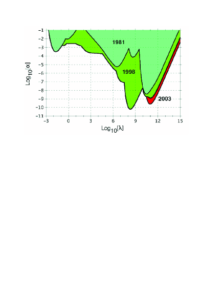
Figure 1: Constraints on a Yukawa modification of Newton law. The colored domains represent, on a log-log plot, the excluded values for amplitude $\alpha$ as a function of the range $\lambda$ (measured in m). Courtesy of the authors of Ref. 18.

The discussion can also be translated into terms bearing on the running constant. To this aim, we rewrite (6) under a form better adapted to the domain $\mathbf{k}\lambda\gg 1$ (which corresponds to $r\ll\lambda$)

$$\widetilde{G}\left[\mathbf{k}\right]=G+\delta\widetilde{G}\left[\mathbf{k}\right]\qquad,\qquad\delta\widetilde{G}\left[\mathbf{k}\right]=-\frac{G\alpha}{\mathbf{k}^{2}\lambda^{2}+1}.$$ (13)

We then expand the anomalous part in this domain

$$\delta\widetilde{G}\left[\mathbf{k}\right]=-\frac{G\alpha}{\mathbf{k}^{2}\lambda^{2}}\left[1+O\left(\frac{1}{\mathbf{k}^{2}\lambda^{2}}\right)\right].$$ (14)

As the constant anomalous acceleration $\delta A$ in (11) with which it is directly associated, the anomalous term $\delta\widetilde{G}\left[\mathbf{k}\right]$ is proportional to the combination $\alpha/\lambda^{2}$. Note that Eqs. (9), (11) and (14), valid in the domain $r\ll\lambda$ (or equivalently $\mathbf{k}\lambda\gg 1$), are sufficient for the purpose of our discussions. At the same time, they have been derived from Eqs. (2), (3) and (6) which are better behaved at the limit of large distances $r\gg\lambda$ (or equivalently $\mathbf{k}\lambda\ll 1$).

V Planetary Tests

Tests of the Newton law bearing either on the third Kepler law or on the precession of the perihelion of planets are known to confirm the validity of general relativity with a good accuracy. We now make the significance of this statement more explicit by writing directly in terms of the anomalous acceleration $\delta A$ the constraints drawn from these tests. Since we study gravity in the outer solar system, we use the Newton theory with the Sun described as a motionless point source. The motion of the probe mass takes place in the central potential (2) and we can write the conservation of energy $E$ and angular momentum $J$

$$\frac{E}{mc^{2}} = \frac{\upsilon_{r}^{2}+\upsilon_{\varphi}^{2}}{2c^{2}}+\Phi\left(r\right)\qquad,\qquad\frac{J}{m}=r\upsilon_{\varphi}$$

$$\upsilon_{r} = \frac{dr}{dt}\qquad,\qquad\upsilon_{\varphi}=r\frac{d\varphi}{dt},$$ (15)

$r$ is the distance from the Sun, $t$ the time coordinate and $\varphi$ the azimutal angle; the trajectory has been assumed to stay in the plane $\theta={\frac{\pi}{2}}$. When eliminating time, we obtain the equation of motion as

$$\frac{d^{2}u}{d\varphi^{2}}+u=-\frac{m^{2}}{J^{2}}r^{2}A\left(r\right)\qquad,\qquad u\equiv\frac{1}{r}.$$ (16)

Note that $r^{2}A\left(r\right)$ can be replaced by $c^{2}\frac{\partial\Phi}{\partial u}$ when $\Phi$ is the potential expressed in terms of the variable $u$.

Using the standard Newton law for the potential ($\alpha=0$), the right hand side in (16) is a constant and the Kepler ellipse is recovered

$$u=\frac{1+e\mathrm{\cos}\varphi}{p}\qquad,\qquad p\equiv a\left(1-e^{2}\right)=\frac{J^{2}}{GMm^{2}}\qquad,\qquad E=-\frac{GMm}{2a}.$$ (17)

The orbital frequency $\omega=\frac{2\pi}{T}$, with $T$ the orbital period, is given by the third Kepler law $\omega^{2}a^{3}=GM$ or, equivalently, by an expression directly drawn from (16)

$$\left[u\right]_{\mathrm{st}}=-\frac{m^{2}}{J^{2}}\left[r^{2}A\right]_{\mathrm{st}}=\frac{GMm^{2}}{J^{2}}.$$ (18)

Here $\left[u\right]_{\mathrm{st}}$ and $\left[r^{2}A\right]_{\mathrm{st}}$ are the values obtained for $u$ and $r^{2}A$ in standard theory.

With the modified Newton law ($\alpha\neq 0$), there is a correction to the third Kepler law (18). If we evaluate it on circular orbits ($e=0$), we obtain in a linear approximation with respect to the small perturbation

$$\frac{u}{\left[u\right]_{\mathrm{st}}}=\frac{r^{2}A}{\left[r^{2}A\right]_{\mathrm{st}}}=1-\frac{r^{2}\delta A\left(r\right)}{GM}.$$ (19)

Consider now a planet, say Mars, for which the elements $a$ or $p$ describing the orbit have been measured through optical means, that is independently of the measurement of the orbital period.Talmadge88 The result obtained for Mars can then be compared with the reference value fixed by the orbit of Earth by forming the ratio $u_{\mathrm{Mars}}/u_{\mathrm{Earth}}$ whose difference to unity now depends on the variation of (19) from Earth to Mars. Defining the relative accuracy $\varepsilon\equiv\left|\delta a/a\right|$ on the element $a$ of Mars as it is measured in AU, we deduce that an anomalous acceleration could be noticed under the condition

$$\varepsilon<\left|\left[\frac{a^{2}\delta A\left(a\right)}{GM}\right]_{\mathrm{Earth}}-\left[\frac{a^{2}\delta A\left(a\right)}{GM}\right]_{\mathrm{Mars}}\right|.$$ (20)

Using (3), this condition is read as a minimum value for the amplitude

$$\frac{\alpha}{\varepsilon}>\frac{1}{\left|\left[\left(1+\frac{a}{\lambda}\right)e^{-\frac{a}{\lambda}}\right]_{\mathrm{Mars}}-\left[\left(1+\frac{a}{\lambda}\right)e^{-\frac{a}{\lambda}}\right]_{\mathrm{Earth}}\right|}.$$ (21)

The curve showing the frontier of the domain is plotted on Fig. 2 with $\log_{10}-\log_{10}$ scales. The range $\lambda$ as well as the radii are measured in AU ($a=1$ for Earth and $1.5$ for Mars). The long range asymptote on the curve corresponds to a fixed value for $\alpha/\lambda^{2}$ and, therefore, for the anomalous acceleration $\delta A$. This point will be discussed in more detail below.

                 

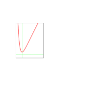
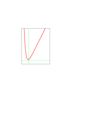
Figure 2: Sensitivity of a Kepler test (left hand part) and precession test (right hand part). The full lines delineate the exclusion domain (above the curve) for the value of the reduced amplitude $\alpha/\varepsilon$ (definitions of $\varepsilon$ given in the text) as a function of $\lambda$ (measured in AU). The logarithms go from -2 to +6 on the horizontal scale and from -1 to +9 on the vertical scale with the zeros indicated by thin lines.

Precise planetary tests are also performed by following the precession of the perihelion of planets.Talmadge88 ; Fischbach98 For simplicity, we evaluate it for an orbit with a low eccentricity $e\ll 1$ in a linear approximation with respect to the small perturbation. In this case, the variable $u$ undergoes a small sinusoidal variation around a constant $1/p\simeq 1/a$ (see Eq. 17). The equation of motion (16) can thus be replaced by an approximation corresponding to the linearization of the associated variation of $r^{2}A\left(r\right)$

$$\frac{d^{2}u}{d\varphi^{2}}+\left(1-2\delta\kappa\right)\left(u-\frac{1}{P}\right)=0$$

$$\delta\kappa=\frac{1}{2}\frac{m^{2}}{J^{2}}\left[r^{2}\frac{\mathrm{d}}{\mathrm{d}r}\left(r^{2}A\left(r\right)\right)\right]_{r=a}=\frac{\alpha a^{2}}{2\lambda^{2}}e^{-\frac{a}{\lambda}}.$$ (22)

The parameter $1/p$ has been replaced by a modified value $1/P$ but this does not matter for our present purpose. What is important for the evaluation of the precession is the modification of the coefficient in front of $u$. It implies that the perihelion (maximum value of $u$) is recovered when $\varphi$ has ran over $2\pi\left(1+\delta\kappa\right)$ rather than the standard value $2\pi$. Defining the relative accuracy $\varepsilon=\left|\delta\varphi/2\pi\right|$ for a test of the precession, we obtain the following relation for the anomaly to be detectable

$$\varepsilon<\alpha\left[\frac{a^{2}}{2\lambda^{2}}e^{-\frac{a}{\lambda}}\right]_{\mathrm{Mars}}.$$ (23)

The frontier of the exclusion domain is drawn as the right hand plot on Fig. 2. It has roughly the same shape as the left hand plot and, in particular, the long range asymptote on the curve corresponds again to a fixed value for $\alpha/\lambda^{2}$.

VI Discussion

As already stated, the Yukawa correction of the Newton law would produce a constant anomalous acceleration over the range of distances probed by Pioneer 10/11 provided the Yukawa range is large enough $\lambda>70~{}\mathrm{AU}$. This means that the tests performed on planets or probes in the solar system correspond to the limit of long ranges $r\ll\lambda$. As shown in the preceding section, this also means that they test a single combination $\alpha/\lambda^{2}$ of the two parameters entering the expression of the Yukawa correction. This entails that it is possible to write the constraints directly in terms of this anomalous acceleration $\delta A$.

This fact is especially clear for the Kepler test since the condition (20) can be rewritten

$$\varepsilon<\left|\frac{\delta A\left(a_{\mathrm{Mars}}\right)}{A\left(a_{\mathrm{Mars}}\right)}-\frac{\delta A\left(a_{\mathrm{Earth}}\right)}{A\left(a_{\mathrm{Earth}}\right)}\right|.$$ (24)

Now $\delta A\left(a\right)$ has essentially the same value at $a=a_{\mathrm{Mars}}$ and $a=a_{\mathrm{Earth}}$ as well as at any distance smaller than the Yukawa range. If we simply denote this constant anomalous acceleration as $\delta A$, we deduce that a test with a relative accuracy $\varepsilon$ is immediately translated into a bound on $\delta A$

$$\left|\delta A\right|<\varepsilon\left|\frac{A_{\mathrm{Earth}}A_{\mathrm{Mars}}}{A_{\mathrm{Earth}}-A_{\mathrm{Mars}}}\right|.$$ (25)

ConsideringAndersonYukawa that the distance to Mars has been tested with an accuracy of the order of 12m, we obtain $\varepsilon\sim 10^{-10}$. Inserting the values of $A_{\mathrm{Mars}}\sim 2.6\times 10^{-3}{\rm m}{\rm s}^{-2}$ and $A_{\mathrm{Earth}}\sim 5.\,9\times 10^{-3}{\rm m}{\rm s}^{-2}$, we deduce that $\delta A$ should remain smaller than $5\times 10^{-13}{\rm m}{\rm s}^{-2}$. This is certainly much smaller than the value (1) needed to explain the Pioneer anomaly.

For the perihelion test, the accuracy (23) can be rewritten in the long range limit $r\ll\lambda$ as

$$\left|\frac{\delta\varphi}{2\pi}\right|=\left|\frac{\delta A\left(a_{\mathrm{Mars}}\right)}{A\left(a_{\mathrm{Mars}}\right)}\right|.$$ (26)

It follows that a test with an accuracy $\left|\delta\varphi\right|$ is again translated into a bound on $\delta A$

$$\left|\delta A\right|<\left|\frac{\delta\varphi}{2\pi}\right|\left|A_{\mathrm{Mars}}\right|.$$ (27)

Both results (25) and (27) constrain the value of $\left|\delta A\right|$ that is also the combination $\alpha/\lambda^{2}$ of the two Yukawa parameters. One can therefore extract the best bound on $\left|\delta A\right|$ from the long range asymptote on the diagram $\left(\lambda,\alpha\right)$ of Fig. 1. This diagram collects the most recent planetary dataCoy03 and it leads to the following bound

$$\delta A\lesssim 3\times 10^{-13}{\rm m}{\rm s}^{-2}.$$ (28)

We can now sum up the present paper as discarding the possibility that the Pioneer anomaly could be explained from a long-range Yukawa deviation from the Newton potential. This conclusionAndersonYukawa has been written directly in terms of the anomalous acceleration $\delta A$ which appears in such a modification of Newton law. The value needed to fit the Pioneer anomaly is in fact more than 1000 times too large to remain unnoticed on tests of the Kepler law or of the precession of perihelions. The discrepancy illustrates the challenge to be met when trying to analyze the Pioneer anomaly in the same framework as other tests of gravity.JaekelTBP

References

- (1) E. G. Adelberger, B. R. Heckel and A. E. Nelson, Ann. Rev. Nucl. Part. Sci. 53, 77 (2003) [hep-ph/0307284] and references in.
- (2) E. Fischbach and C. Talmadge, The Search for Non Newtonian Gravity (AIP Press/Springer Verlag, New York, 1998) and references in.
- (3) C. M. Will, Living Reviews in Relativity 4, 4 (2001) and references in.
- (4) C. D. Hoyle et al, Phys. Rev. Lett. 86, 1418 (2001); Phys. Rev. D70, 042004 (2004).
- (5) J. Long et al, Nature 421, 922 (2003).
- (6) J. Chiaverini et al, Phys. Rev. Lett. 90, 151101 (2003).
- (7) S. K. Lamoreaux, Phys. Rev. Lett. 78, 5 (1997).
- (8) U. Mohideen and A. Roy, Phys. Rev. Lett. 81, 4549 (1998); B. W. Harris, F. Chen and U. Mohideen, Phys. Rev. A62, 052109 (2000).
- (9) T. Ederth, Phys. Rev. A62, 062104 (2000).
- (10) H. B. Chan et al, Science 291 1941 (2001); Phys. Rev. Lett. 87, 211801 (2001).
- (11) G. Bressi et al, Phys. Rev. Lett. 88, 041804 (2002).
- (12) R. S. Decca et al, Phys. Rev. Lett. 91, 050402 (2003).
- (13) M. Bordag, U. Mohideen and V. M. Mostepanenko, Phys. Rep. 353, 1 (2001).
- (14) A. Lambrecht and S. Reynaud, in Poincaré Seminar 2002, ed. B. Duplantier and V. Rivasseau (Birkhaüser Verlag, Basel, 2003), p. 109.
- (15) R. S. Decca et al, Phys. Rev. D68, 116003 (2003).
- (16) F. Chen et al, Phys. Rev. A69, 022117 (2004).
- (17) C. Talmadge et al, Phys. Rev. Lett. 61, 1159 (1988).
- (18) J. Coy, E. Fischbach, R. Hellings, C. Talmadge and E. M. Standish, private communication (2003).
- (19) J. G. Williams, X. X. Newhall and J. O. Dickey, Phys. Rev. D53, 6730 (1996).
- (20) R. D. Reasenberg et al, Astrophys. J. 234, L219 (1979).
- (21) R. Hellings et al, Phys. Rev. Lett. 51, 1609 (1983).
- (22) J. D. Anderson et al, Astrophys. J. 459, 365 (1996).
- (23) N. I. Kolosnitsyn and V. N. Melnikov, gr-qc/0302048.
- (24) J. D. Anderson et al, Phys. Rev. Lett. 81, 2858 (1998).
- (25) J. D. Anderson et al, Phys. Rev. D65, 082004 (2002).
- (26) J. D. Anderson, M. M. Nieto and S. G. Turyshev, Int. J. Mod. Phys. D11, 1545 (2002).
- (27) J. D. Anderson et al, Mod. Phys. Lett. A17, 875 (2003).
- (28) M. M. Nieto and S. G. Turyshev, Class. Quantum Grav. 21, 4005 (2004).
- (29) S. G. Turyshev, M. M. Nieto and J. D. Anderson, gr-qc/0409117.
- (30) T. Goldman, J. Pérez-Mercader, F. Cooper and M. M. Nieto, gr-qc/9210005.
- (31) P. D. Mannheim, Astrophys. J. 479, 659 (1997).
- (32) M. Milgrom, New Astr. Rev. 46, 741 (2002).
- (33) R. H. Sanders and S. S. McGaugh, astro-ph/0204521.
- (34) A. Aguirre et al, Class. Quantum Grav. 18, R223 (2001); A. Aguirre, astro-ph/0310572.
- (35) S. M. Carroll et al, Phys. Rev. D70, 043528 (2004).
- (36) A. D. Sakharov, Doklady Akad. Nauk 177, 70 (1967) [Sov. Phys. Doklady 12, 1040 (1968)]; R. J. Adler, Rev. Mod. Phys. 54, 729 (1982).
- (37) G. Dvali, A. Gruzinov and M. Zaldarriaga, Phys. Rev. D68, 024012 (2003).
- (38) M. Reuter and H. Weyer, hep-th/0410119.
- (39) See the section XI-B in Ref. 25.
- (40) M.-T. Jaekel and S. Reynaud, gr-qc/0410148.