Observable form of pulses emitted from relativistic collapsing objects

Abstract

In this work, we discuss observable characteristics of the radiation emitted from a surface of a collapsing object. We study a simplified model in which a radiation of massless particles has a sharp in time profile and it happens at the surface at the same moment of comoving time. Since the radiating surface has finite size the observed radiation will occur during some finite time. Its redshift and bending angle are affected by the strong gravitational field. We obtain a simple expression for the observed flux of the radiation as a function of time. To find an explicit expression for the flux we develop an analytical approximation for the bending angle and time delay for null rays emitted by a collapsing surface. In the case of the bending angle this approximation is an improved version of the earlier proposed Beloborodov-Leahy-approximation. For rays emitted at $R>2R_{g}$ the accuracy of the proposed improved approximations for the bending angle and time delay is of order (or less) than 2-3$\%$. By using this approximation we obtain an approximate analytical expression for the observed flux and study its properties.

I Introduction

Neutron stars and black holes are compact relativistic objects. Light propagating in the vicinity of such objects is affected by a strong gravitational field. For the description of the photon propagation under these conditions the general relativity is required. This is evident for black holes where the gravitational potential at the horizon (in the $c^{2}$ units) is of order of 1. Though a value of the gravitational potential at a surface ($R_{NS}\sim 8M_{\odot}$) of neutron stars ($M_{NS}\sim 1.5M_{\odot}$) lp1 is smaller and is of order of $\sim 0.2$, it was demonstrated recently that general relativistic effects might be important for understanding the features of the radiation coming from these objects pfc -bel . In particular, one of the explanations of X-ray bursts is connected with possible explosions of the matter which is accumulated on the surface of a neutron star entering in a binary system as a result of “sucking” the matter from a usual-star companion. It was shown (see ll , mr , clm ) that the profile of the X-ray-curve observed by a distant observer can be explained only if the effects of general relativity are taken into account. In particular, according to the general relativity, because of the gravitational bending of light rays, a distant observer can see a part of the opposite side of the neutron star which is invisible in a flat spacetime. The radiation emitted from this part gives an important contribution and has a visible impact on the form of the signal from the X-ray burst.

The effects of the general relativity also modify considerably light curves for continuous in time radiation from the surface of a collapsing star as seen by a distant observer. These effects were studied in detail by Ames and Thorne at , Jaffe jaffe and Lake lr . In this study main attention was focused on the details connected with light emitted near (unstable) circular photon orbits at $3r_{g}/2$, where $r_{g}$ is a gravitational radius of a collapsing star. In such considerations there were usually adopted a number of simplifying assumptions, such as: (1) Spherical geometry; (2) Dust-like (pressure free) equation of state; (3) Radiation comes only from the (free-falling) surface of the star; and (4) It is continuous in time.

In this paper we would like to discuss a slightly different set up, when the assumption (4) is violated. Namely we assume that the radiation emitted from the surface of a collapsing spherically symmetric stellar object has a profile of a sharp in time pulse. Such radiation may occur in different situations. For example, suppose a neutron star or a proto-neutron star looses its stability as a result of the accretion of matter onto it or due to the softening of equation of state kaon at the center which is supposed to be already several times higher than the nuclear density . During the collapse, the matter density of a compact object is growing and the whole system evolves into the much higher density than the normal nuclear density sha –nsc , beyond which new hadronic phase transitions might take place schafer . One might expect a possible sharp-in-time emission of massless particles (photons and neutrino) during such phase transition vro .

Since at the moment there are a lot of theoretical uncertainties in the estimations and detailed description of these processes, we shall study a simplified (toy) model. Namely we assume that a radiation of massless particles has a sharp in time pulse profile and it happens at the surface at the same instant of time (from a point of view of a comoving observer). The time required for the radiation to reach a distant observer depends on the position of a radiative region on the collapsing surface. For this reason the pulse emission results in a continuous flux received by the observer during some finite interval of time. During this interval the flux as well as the redshift factor changes. In principle, knowing the redshift and light curves allows one to obtain direct information about the collapsing body at the moment when the radiation occurs. We shall demonstrate that if the emission occurs at the moment when the radius of a collapsing body is $R>4.5M$, the observed characteristics of the pulse radiation with a very high accuracy can be written in an explicit form in terms of elementary functions. We shall use this result to study how different (gravitational redshift, Doppler and focusing) effects affect the form of redshift and light curves.

In section 2 we consider null rays emitted from a surface of a spherical collapsing object. The equations of motion of the freely collapsing surface and for rays propagating in the surrounding Schwarzschild geometry are well known. In order to fix the notations we collect the required formulas in section 2 in the form they are used in the further sections. The time of arrival of null rays emitted by a collapsing surface and their bending angle are given by elliptic integrals. In section 3, we propose an explicit analytic expressions which approximate these quantities with very high accuracy. For rays emitted at $R>2R_{g}$ this accuracy is of order (or less) than 2-3$\%$. This approximation is used to obtain the expressions for the intensity and flux for a short flash observed by a distant observer (section 4). The results of numerical calculations of the redshift, bending angle and light curves are given in section 5. In section 6, the results are summarized and discussed.

II Basic Equations

II.1 Freely-falling spherical surface

We consider a photon emitted from a collapsing spherical surface and propagating to the observer at infinity in the background of Schwarzschild metric

$$ds^{2}=-fdt^{2}+f^{-1}dr^{2}+r^{2}d\Omega\,,$$ (1)

$$f=f(r)=1-2M/r\,,$$ (2)

where $M$ is the mass of the collapsing object. We adopt the natural units, $c=G=\hbar=1$. In at and sha the motion of a spherical surface during the gravitational collapse was discussed under assumption that the dynamical role of the pressure can be neglected. We also use the dust-like equation of state so that a solution for the interior of the collapsing object is a well known Tolman solution tolmann , while the surface follows a radial geodesic in the Schwarzchild geometry os .

Denote by $\tau$ the proper time as measured by an observer comoving with the collapsing surface. We suppose that the collapse starts at $\tau=0$ and the initial surface radius is $R_{0}$. Then, in the parametric form (using the conformal time parameter $\eta$), the equation of motion of the surface is

$$R = \frac{R_{0}}{2}(1+\cos\eta),$$ (3)

$$\tau = \sqrt{\frac{R_{0}^{3}}{8M}}(\eta+\sin\eta)\,\,.$$ (4)

In the same parametric form the Schwarzschild time $t^{(e)}$ corresponding to the proper time $\tau$ at the surface is

$$t^{(e)} = 2M\ln\left|\frac{\sqrt{R_{0}/2M-1}+\tan(\eta/2)}{\sqrt{R_{0}/2M-1}-\tan(\eta/2)}\right|$$ (5)

$$+2M\sqrt{R_{0}/2M-1}[\eta+\frac{R_{0}}{4M}(\eta+\sin\eta)]\,.$$

We assumed that $t^{(e)}(\tau=0)=0$.

We denote

$$v_{i}=f^{-1}(R)\frac{dR}{dt}\,.$$ (6)

This quantity has the meaning of the invariant radial velocity. Then in a general case the four-velocity of the collapsing surface is

$$v^{\mu}=(dt^{(e)}/d\tau,dR/d\tau,0,0)\,,$$ (7)

where

$${dt^{(e)}\over d\tau}={1\over\sqrt{f(R)}\sqrt{1-v_{i}^{2}}}\,,$$ (8)

$${dR\over d\tau}=v_{i}f(R){dt^{(e)}\over d\tau}={\sqrt{f(R)}v_{i}\over\sqrt{1-v_{i}^{2}}}\,.$$ (9)

Using eq.(3) and (5), we obtain the following expression for the velocity $v_{i}$ of a freely falling surface with the initial radius $R_{0}$ at the moment when its radius is $R$

$$v_{i}=-\sqrt{\frac{2M}{R}}\frac{\sqrt{1-R/R_{0}}}{\sqrt{1-2M/R_{0}}}\,.$$ (10)

We also have

$${dt^{(e)}\over d\tau}={\sqrt{1-2M/R_{0}}\over 1-2M/R}\,,$$ (11)

$${dR\over d\tau}=-\sqrt{2M/R}\sqrt{1-R/R_{0}}\,.$$ (12)

II.2 Propagation of null rays emitted from the surface

Consider a photon emitted from the surface. Its trajectory lies in the plane. Without loss of generality we assume that it coincides with a plane of the fixed coordinate $\phi$, so that the vector of the 4-momentum of the photon is

$$p^{\mu} = (p^{t},p^{r},p^{\theta},0)\,.$$ (13)

Because of the symmetry of the Schwarzschild metric, $E=-p_{t}$ (the energy at infinity) and $L=p_{\theta}$ (the angular momentum) are constants of motion. Instead of the angular momentum $L$ we shall use the impact parameter

$$l=L/E\,.$$ (14)

The radial momentum $p^{r}$ is

$$p^{r}=\sigma EZ\,,$$ (15)

where

$$Z=Z(l,r)=\sqrt{1-l^{2}f(r)/r^{2}}\,.$$ (16)

Here and later $\sigma$ denotes a sign function which takes the values $+$ and $-$ for a forward ($p^{r}>0$) and backward ($p^{r}<0$) emission, respectively.

There is an upper limit for the impact parameter, $l_{max}$, for a photon which being emitted from a surface of radius $R$ reaches the infinity:

$$l_{max}=\frac{R}{\sqrt{f(R)}}.$$ (17)

Suppose a null ray emitted by a collapsing surface reaches the infinity at $\theta=0$ and has the impact parameter $l$. Then the emission angle, $\beta$, as measured by an observer comoving with the surface, is defined by the relation

$$\cos\beta_{\sigma}(l,R)=\frac{\sigma Z(l,R)-v_{i}}{1-\sigma v_{i}Z(l,R)}\,.$$ (18)

We consider only the light emitted with $\beta\leq\pi/2$. A tangentially emitted photon with respect to a comoving observer($\beta=\pi/2$), for a collapsing surface ($v_{i}<0$), is possible only for a backward emission. The corresponding impact parameter $l=l_{T}$ is determined by the condition

$$Z=-v_{i}\,.$$ (19)

Solving this equation one obtains

$$l_{T}=\frac{R}{\sqrt{1-2M/R_{0}}}\,.$$ (20)

For $R=3\sqrt{3}\sqrt{1-2M/R_{0}}M$ the parameter $l_{T}$ is equal to $3\sqrt{3}$, the value corresponding to the (unstable) circular photon orbit. To escape delicacies connected with more complicated behavior of the photons near this orbit we assume that $R>3\sqrt{3}\sqrt{1-2M/R_{0}}M$. In this case for a photon which reaches the infinity the possible ranges of an impact parameter are $0\leq l\leq l_{max}$ and $l_{T}\leq l\leq l_{max}$ for a forward and backward emission, respectively. A discussion of the allowed ranges of the impact parameter for the smaller radius up to $R\sim 2M$, can be found in at and jaffe .

II.3 Redshift

Let $p_{\mu}^{(e)}$ be 4-momentum of a photon emitted by a collapsing surface which has 4-velocity $v^{(e)\mu}$. Then $\nu^{(e)}=-p_{\mu}^{(e)}v^{(e)\mu}$ is the frequency of the photon as measured by a comoving to the surface observer. Since an observer at infinity is at rest, its 4-velocity is $v^{(o)\mu}=\delta^{\mu}_{0}$ and the observed frequency of the photon is $\nu^{(o)}=-p_{\mu}^{(o)}v^{(o)\mu}$, where $p_{\mu}^{(o)}$ is the 4-momentum of the photon at infinity. For a given ray, the redshift factor $\Phi$ is defined as the ratio of the emitted frequency $\nu^{(e)}$ to the observed at infinity frequency $\nu^{(o)}$

$$\Phi={\nu^{(e)}\over\nu^{(o)}}\,.$$ (21)

For a ray with the impact parameter $l$ emitted from the surface of the radius $R$ one has

$$\Phi_{\sigma}(l,R)={1-\sigma v_{i}Z(l,R)\over\sqrt{f}\sqrt{1-v_{i}^{2}}}\,.$$ (22)

For a freely falling surface we get

$$\Phi_{\sigma}(l,R)=\frac{\sqrt{1-2M/R_{0}}}{1-2M/R}$$ (23)

$$\times\left[1+\sigma\sqrt{\frac{(2M/R)(1-R/R_{0})}{1-2M/R_{0}}}Z(l,R)~{}\right].$$

II.4 Bending angle

We use the freedom in the choice of spherical coordinates to put the angle $\theta$ in the direction to an observer at infinity to be equal to zero, $\theta^{(o)}=0$. Consider a null ray emitted by the collapsing surface when its radius is $R$ and which reaches the distant observer. Suppose its impact parameter is $l$. Then such a ray is emitted by the collapsing surface from the region at the angle $\theta^{(e)}$. For forward emission this bending angle is

$$\theta_{+}^{(e)}=\Theta(l,R)\,,$$ (24)

$$\Theta(l,R)=l\int^{\infty}_{R}\frac{dr}{r^{2}Z(l,r)}\,.$$ (25)

For a backward-emission a photon before it reaches the infinity should pass through a turning point, $r_{t}<R$, which is determined by $Z(l,r_{t})=0$, or

$$r_{t}^{2}/(1-2M/r_{t}) = l^{2}.$$ (26)

One can see that, for $l=l_{max}=R^{2}/(1-2M/R)$, $r_{t}=R$ as expected. Then we get

$$\theta_{-}^{(e)}=2\Theta(l,r_{t})-\Theta(l,R)\,.$$ (27)

II.5 Arrival time

Consider a null ray with the impact parameter $l$ emitted from the collapsing surface at the moment $\tau$ when it has the radius $R(\tau)$. Denote by $t_{\pm}^{(o)}$ the time when it reaches a distant observer at radius $r^{(o)}$ for the forward/backward ray. One has

$$t^{(o)}_{+}(l,\tau)=t^{(e)}(\tau)+\int^{r_{0}}_{R(\tau)}\frac{dr}{f(r)Z(l,r)},$$ (28)

$$t^{(o)}_{-}(l,\tau)=t^{(e)}(\tau)+2\int^{r_{0}}_{r_{t}}\frac{dr}{f(r)Z(l,r)}-\int^{r_{0}}_{R(\tau)}\frac{dr}{f(r)Z(l,r)}.$$ (30)

It is evident that $t^{(o)}\to\infty$ when $r_{0}\to\infty$. For this reason it is more convenient to consider a finite quantity, the time difference between arrival of two null rays emitted at two different moments of proper time, $\tau$ and $\tau_{e}$, respectively. For the second ray, emitted at $\tau_{e}$, we put $l=0$. Such a ray goes radially. We denote this time difference by $\Delta t(l;\tau,\tau_{e})$. In the limit when $r^{(o)}\to\infty$ this quantity remain finite. For the forward ray it is given by the following expression

$$\Delta t_{+}(l;\tau,\tau_{e})=t^{(e)}(\tau)-t^{(e)}(\tau_{e})+T(l,R(\tau))$$

$$+R(\tau_{e})-R(\tau)+2M\ln\frac{R(\tau_{e})-2M}{R(\tau)-2M},$$ (31)

where

$$T(l,R)\equiv\int^{\infty}_{R}\frac{dr}{f(r)}\left[\frac{1}{Z(l,r)}-1\right]\,.$$ (32)

Similarly for the backward ray one has

$$\Delta t_{-}(l;\tau,\tau_{e})=t^{(e)}(\tau)-t^{(e)}(\tau_{e})+2T(l,r_{t})-T(l,R(\tau))$$ (33)

$$+R(\tau_{e})+R(\tau)-2r_{t}+2M\ln\frac{(R(\tau)-2M)(R(\tau_{e})-2M)}{(r_{t}-2M)^{2}}.$$

The integrals for $\Theta$ and $T$ (see relations (25) and (32), respectively) can be expressed in terms of the elliptic functions. However, for practical calculations it is very convenient to have approximations for these quantities in terms of simple elementary functions. In the next section, we develop high accuracy analytic approximations, for the integrals $\Theta(l,R)$ and $T(l,R)$.

III Analytic Approximation

III.1 Approximation for bending angle

It is convenient to use the dimensionless quantities

$$x=M/r\,,\hskip 14.22636ptq\equiv M/R\,,\hskip 14.22636pt\hat{l}=l/M\,.$$ (34)

We also denote

$$\hat{Z}=\hat{Z}(\hat{l},q)=\sqrt{1-\hat{l}^{2}q^{2}(1-2q)}\,,$$ (35)

so that

$$Z(l,R)=\hat{Z}(\hat{l},M/R)\,.$$ (36)

Using these notations the integral $\Theta$, (25), can be written in the form

$$\Theta=\int^{q}_{0}dx{\hat{l}\over\hat{Z}(\hat{l},x)}\,.$$ (37)

As already was mentioned, for a given surface radius $R$ there exists a critical value $\hat{l}_{\max}=1/(q\sqrt{1-2q})$ and the rays emitted from this surface must have $|\hat{l}|\leq\hat{l}_{max}$. For a fixed $q$ and $\hat{l}\in[0,\hat{l}_{max}]$ the function $\hat{Z}$ changes from 1 to 0.

In a flat metric with $f=1$, one can calculate the integral (37) analytically to get

$$\Theta_{flat}=\arccos(\sqrt{1-\hat{l}^{2}q^{2}}).$$ (38)

Leahy ll discovered that in a wide range of its arguments the exact integral for the bending angle can be approximated by a simple analytical expression. A simple elegant form of the approximative expression was proposed later by Beloborodov bel . In the notations adopted in the present paper this formula reads

$$1-\cos\beta=(1-\cos\theta^{(e)})(1-2M/R)\,,$$ (39)

where $\beta$ is defined by (18). It is easy to show that this relation corresponds to the following approximation for $\Theta$

$$\Theta_{0}=\arccos\left[{\hat{Z}-2q\over 1-2q}\right]\,\,.$$ (40)

We shall refer to this relation as to Beloborodov–Leahy (or BL–) approximation.

The typical accuracy of the BL–approximation is of order of 1% for the light rays emitted from the surface $R=6M$. For this reason it works well in the study of light emitted from a surface of a neutron star bel . In a recent paper clm BL-approximation was used for fitting the light curves of X-ray pulsars. For smaller $R$ the accuracy of the BL–approximation is worse. For example it becomes of order of 10% for $R=4M$. In order to use this approximation for our purposes we first slightly modify it to improve the accuracy.

To improve the BL-approximation, let us compare expansions of $\Theta$ and $\Theta_{0}$ at small values of $\hat{l}$. We have

$$\Theta=q\hat{l}+{1\over 12}(2-3q)q^{3}\,\hat{l}^{3}$$

$$+{1\over 280}(21-70q+60q^{2})q^{5}\,\hat{l}^{5}+\ldots\,,$$ (41)

$$\Theta_{0}=q\hat{l}+{1\over 12}(2-3q)q^{3}\,\hat{l}^{3}$$

$$+{1\over 480}(36-120q+105q^{2})q^{5}\,\hat{l}^{5}+\ldots\,.$$ (42)

($\ldots$ denotes terms of higher order in $\hat{l}$.) This gives

$$\Theta-\Theta_{0}=-{1\over 224}q^{7}\hat{l}^{5}+\ldots\,.$$ (43)

We write our ansatz as follows

$$\hat{\Theta}(\hat{l},q)=\arccos\left[{\hat{Z}(\hat{L},q)-2q\over 1-2q}\right]+b_{5}q^{2}{\cal Z}^{5}\,.$$ (44)

where

$${\cal Z}\equiv{1-\hat{Z}(\hat{l},q)\over 1-2q}.$$ (45)

For small $\hat{l}$

$${\cal Z}={1\over 2}q^{2}\,\hat{l}^{2}+{1\over 16}(2-3q)\,q^{4}\hat{l}^{4}+\ldots\,.$$ (46)

We write $b_{5}$ as follows

$$b_{5}=-{\beta 2^{5/2}\over 224}\,.$$ (47)

For $\beta=1$ this expression correctly reproduces the expansion of $\Theta(l,q)$ for small $q$ up to the terms of the order of $O(q^{7})$. Numerical calculations show that the accuracy of the approximation is very good for the following choice

$$\beta=3.5\,,\hskip 8.5359ptb_{5}=0.0884\,.$$ (48)

Thus the approximate expression for the forward-emitted rays is

$$\theta^{(e)}_{f}\approx\hat{\Theta}(l,q=M/R)\,,$$ (49)

where $\hat{\Theta}$ is given by (44), (47), and (48). The relative error $\Delta_{\theta}=(\theta_{f}^{(e)}-\hat{\Theta})/\theta^{(e)}$ of the approximate expression is very small. It is less than 0.5% for $R\geq 4.5M$ for all the allowed values of $l$. Figure 1 shows the quantity $D=10^{3}\times\Delta_{\theta}$ as a function of $s=l/l_{max}(q)$, where $q=M/R$. The parameter $s$ is chosen so that for every value $q$ and the impact parameter $l$ from $0$ to its maximum allowed value $l_{max}$ the value of $s$ belongs to the same interval $[0,1]$. For $R=4M$ the error $\Delta_{\theta}$ is slightly larger. It is still less than 0.8 % every where excluding a narrow vicinity of $s=1$ where it reaches 2%.

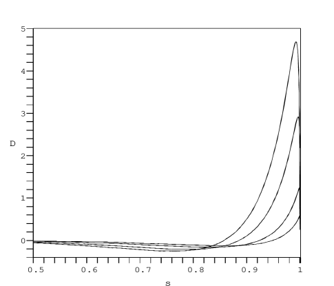
Figure 1: The figure shows $D=10^{3}\Delta_{\theta}$ ($\Delta_{\theta}$ is a relative error for $\Theta$) as a function of $s=l/l_{max}$. The plots are shown for the following 4 values of $R/M=4.5,5,6,7$ (the smaller value $R/M$ the higher is a plot in the vicinity of $s=1$). The curves are practically indistinguishable from $D=0$ line for $s<0.5$. For this reason we plotted only $s\geq 0.5$ parts of the graphs.

We shall use the formula (44) to approximate the bending angle for the forward emission. For the backward emission the approximate formula is

$$\theta^{(e)}_{b}(l,R)\approx 2\hat{\Theta}(\hat{l},M/r_{t})-\hat{\Theta}(\hat{l},M/R)\,,$$ (50)

where $r_{t}$ is defined by (26).

III.2 Approximation for arrival time

Now we consider the arrival time. Using the dimensionless version of $T$, ${\cal T}=T/M$, we can rewrite the expression (32) in the following form:

$${\cal T}={\cal T}(\hat{l},q)=\int^{q}_{0}dx{\hat{l}^{2}\over\hat{Z}(\hat{l},x)(1+\hat{Z}(\hat{l},x))}\,.$$ (51)

We want to obtain an analytic approximation for $T$.

Let us first assume that the function $f$ which enters $Z$ changes slowly, and put $f=$const in the integral (51). This integral can be calculated exactly

$${\cal T}_{0}={1-\sqrt{1-\hat{l}^{2}\,q^{2}\,f}\over f\,q}\,.$$ (52)

We restore the dependence $f$ on $q$ and use this expression with $f=1-2q$ as a starting point for our approximation. The corresponding expression can be written as

$${\cal T}_{0}={{\cal Z}\over q}\,.$$ (53)

One can check that this approximation is very good for small $q$.

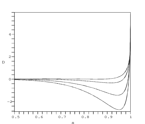
Figure 2: The figure shows $D=10^{3}\Delta_{T}$ ($\Delta_{T}$ is a relative error for $T$) as a function of $s=l/l_{max}$. The plots are shown for the following 4 values of $R/M=4.5,5,6,7$ (the smaller value $R/M$ the lower is a plot in the vicinity of $s=1$). The curves are practically indistinguishable from $D=0$ line for $s<0.5$. For this reason we plotted only $s\geq 0.5$ parts of the graphs.

To improve it, let us compare expansions of ${\cal T}$ and ${\cal T}_{0}$ at small values of $\hat{l}$. We have

$${\cal T}={1\over 2}q\,\hat{l}^{2}+{1\over 8}(q^{3}-2q^{4})\,\hat{l}^{4}+\ldots\,,$$ (54)

$${\cal T}_{0}={1\over 2}q\,\hat{l}^{2}+{1\over 16}(2q^{3}-3q^{4})\,\hat{l}^{4}+\ldots\,.$$ (55)

This gives

$${\cal T}-{\cal T}_{0}={1\over 16}q^{4}\hat{l}^{4}+\ldots\,.$$ (56)

Our ansatz for the improved approximation is

$$\hat{\cal T}={\cal T}_{0}+Q({\cal Z})\,.$$ (57)

Using (46) one can conclude that in order to provide the correct $q^{4}\hat{l}^{4}$ behavior of the correction at small $\hat{l}$ the function $Q$ must have the following expansion

$$Q({\cal Z})={1\over 4}{\cal Z}^{2}+\ldots\,.$$ (58)

We write our ansatz as follows

$$Q({\cal Z})={1\over 4}{\cal Z}^{2}+a_{3}{\cal Z}^{3}+a_{4}{\cal Z}^{4}\,.$$ (59)

Numerical calculations show that the accuracy of the approximation is very good for the following choice of the parameters

$$a_{3}=1/15\,,\hskip 14.22636pta_{4}=1/25\,.$$ (60)

Thus the approximation for the time delay takes the form

$$\hat{\cal T}={{\cal Z}\over q}+Q({\cal Z})\,,\hskip 8.5359ptQ({\cal Z})={1\over 4}{\cal Z}^{2}+{1\over 15}{\cal Z}^{3}+{1\over 25}{\cal Z}^{4}\,,$$ (61)

$$\hat{T}(l,R)=M\hat{\cal T}(\hat{l},M/R)\,.$$ (62)

The relative error $\Delta_{T}=(T-\hat{T})/{T}$ of the approximate expression is again very small. It is less than 0.5% for $R\geq 4.5M$ for all the allowed values of $l$. Figure 2 shows the quantity $D=10^{3}\times\Delta_{T}$ as a function of $s=l/l_{max}$. For $R=4M$ the error $\Delta_{T}$ is slightly larger. It is still less than 1 % every where excluding a narrow vicinity of $s=1$ where it reaches 3%.

For the calculations of the intensity of the light from a radiating body observed at infinity we shall need the expression for the derivatives $\hat{\cal T}_{,q}$ and $\hat{\cal T}_{,\hat{l}}$. The first one can be easily found from the definition of ${\cal T}$ (51)

$$\hat{\cal T}_{,q}={\hat{l}^{2}\over\hat{Z}(\hat{l},x)(1+\hat{Z}(\hat{l},x))}\,.$$ (63)

For the derivative $\hat{\cal T}_{,\hat{l}}$ we shall use the approximate expression obtained by the differentiation of $\hat{\cal T}$ given by (61) with respect to $\hat{l}$. The approximation for the derivative $\hat{\cal T}_{,\hat{l}}$ works slightly worse than the approximation for $\hat{\cal T}$. We denote

$$\Delta_{T_{,l}}=({\cal T}_{,\hat{l}}-\hat{\cal T}_{,\hat{l}})/{\cal T}_{,\hat{l}}$$ (64)

the relative error. The figure 3 shows $D=10^{2}\Delta_{T_{,l}}$ as a function of $s=l/l_{max}$. The maximum value of the error (for $R=4.5M$) is near $s=1$ and it reached 5%.

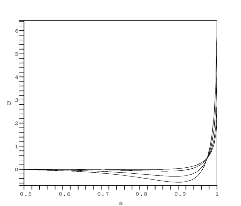
Figure 3: The figure shows $D=10^{2}\Delta_{T_{,l}}$ ($\Delta_{T_{,l}}$ is a relative error for $T_{,l}$) as a function of $s=l/l_{max}$. The plots are shown for the following 4 values of $R/M=4.5,5,6,7$. In the region where $D<0$, the smaller value $R/M$ the lower is a plot in the vicinity of $s=1$. The curves are practically indistinguishable from $D=0$ line for $s<0.5$. For this reason we plotted only $s\geq 0.5$ parts of the graphs.

IV A short flash from a collapsing surface

IV.1 Flux and intensity for a short flash

We shall use superscripts $(e)$ and $(o)$ for emitted and observed radiation, respectively. To characterize such a radiation one uses the notions of the flux and intensity. The flux, $F$, is a power of the radiation per unit area emitted by a radiating surface or received by the detector. The intensity, $I$, is a power of either emitted or observed radiation per unit area per unit solid angle. Quite often the spectral characteristics, called the specific flux, ${\cal F}_{\nu}$, and specific intensity, ${\cal I}_{\nu}$, are also used. They are ”per unit frequency” versions of $F$ and $I$, respectively. Evidently, one has

$$F=\int d\nu{\cal F}_{\nu}\,,\hskip 8.5359ptI=\int d\nu{\cal I}_{\nu}\,.$$ (65)

The intensity $I$ and specific intensity ${\cal I}_{\nu}$ depend on the angle $\theta$ between the direction of radiation and the normal to emitting (observing) area. The flux and specific flux are obtained by integration of these quantities over the directions

$$F=\int d\Omega I\,,\hskip 8.5359pt{\cal F}_{\nu}=\int d\Omega{\cal I}_{\nu}\,,$$ (66)

where $d\Omega$ is an element of a solid angle. For an isotropic case with azimuthal symmetry,

$$d\Omega=2\pi\sin\theta d\theta\,.$$ (67)

The observed intensity $I^{(o)}$ depends on the direction, or (in our case) on the angle $\theta$ between the normal to the detector surface and the direction of observation. Instead of the direction angle $\theta$ one can use the impact parameter $l$ of an incoming photon. For large $r_{0}$ one has $\theta=l/r_{0}$, and $d\Omega^{(o)}=2\pi ldl/r^{2}_{0}$. Thus the relation (66) can be written as remark

$$F^{(o)}=\int ldl{2\pi I^{(o)}\over r_{0}^{2}}\,.$$ (68)

In the integrand, the intensity $I^{(o)}$ is now considered as a function of impact parameter $l$: $I^{(o)}=I^{(o)}(l)$.

The impact parameter $l$ is conserved along the photon trajectory. It specifies the trajectory itself. Thus for a given value $l$ one can determine both, the bending angle $\theta^{(e)}$ (the angle on the surface of a collapsing body where the ray was emitted) and the angle $\beta$ at which it was emitted.

One can show (see e.g. Exercise 22.17 in mtw ), that the quantity $I_{\nu}(\nu)/\nu^{3}$ remains constant along a photon’s world line. This quantity is proportional to the number density in phase space for photons and its conservation follows from the Liouville’s theorem (see e.g., at and pod ).

Consider a light ray with the impact parameter $l$ emitted from the collapsing surface at the moment of the proper time $\tau$, and let $t$ be the time when it reaches a distant observer at $r_{0}$. For fixed $r_{0}$ relations (28) and (30) can be used to determine $\tau=\tau(t,l)$.

The specific flux as measured by a distant observer at time $t$ is

$${\cal F}^{(o)}_{\nu_{0}}(t)={2\pi\over r_{0}^{2}}\int ldl\Phi^{-3}{\cal I}_{\nu_{e}}^{(e)}(l,\nu_{e},\tau(t,l))\,.$$ (69)

Here $\Phi=\Phi(l,R)$ is given by eq.(22), and $R$ is the radius of the collapsing surface at the moment when a null ray with the impact parameter $l$ leaves it in order to reach the observer at $r_{0}$ at the moment $t$. We denote by $\tau$ the corresponding proper time on the surface. For a fixed time of arrival, $t$, and the moment of emission $\tau$, one can use the relations (28) and (30) to determine the corresponding value of the impact parameter $l=l_{t}(\tau)$. Thus the integral over $l$ in eq.(69) can be rewritten as an integral over the proper time, $\tau$:

$${\cal F}^{(o)}_{\nu_{0}}(t)=\frac{2\pi}{r_{0}^{2}}\int d\tau W\Phi^{-3}{\cal I}_{\nu_{e}}^{(e)}(l,\nu_{e},\tau)\,,$$ (70)

where

$$W\equiv l\left|dl\over d\tau\right|\,.$$ (71)

The expression for $W$ can be obtained by differentiating eq.(28) and eq.(30) with respect to $\tau$ for a fixed value of $t^{(o)}_{\sigma}$. Using the analytic approximations for the arrival time, we get (for details see Appendix)

$$W={\cal J}^{-1}_{\sigma}\,|Z-\sigma v_{i}|R{dt^{(e)}\over d\tau}\,.$$ (72)

Here $dt^{(e)}/d\tau$ is given by (11), and

$${\cal J}_{+}=1+\frac{M}{R}Q^{\prime}({\cal Z})\,,$$ (73)

$${\cal J}_{-}={\cal J}_{+}+{4MRZ\over r_{t}^{2}}\frac{(r_{t}+MQ^{\prime}_{r_{t}})}{r_{t}-3M}\,.$$ (74)

Here $Q^{\prime}_{r_{t}}=Q^{\prime}(f^{-1}(r_{t}))$, $Z=Z(l,R)$, ${\cal Z}={\cal Z}(l,R)$, and $\Phi=\Phi(l,R)$, and the arguments in these functions are $l=l_{t}(\tau)$ and $R=R(\tau)$. We also use a notation $Q^{\prime}=dQ/d{\cal Z}$. A transition from the forward to the backward ray regime occurs at the point where $Z=0$ that is at $l=l_{max})$. It is easy to see that at this point $W_{-}=W_{+}$, as it is expected.

We shall need an explicit form of $W$ for a special case when a ray is emitted radially and hence $l=0$. In this case only forward emission is possible and we have ${\cal J}_{+}=1$. Thus the corresponding value $W_{0}$ takes the form

$$W_{0}=\left[1+\sqrt{\frac{2M}{R}}\frac{\sqrt{1-R/R_{0}}}{\sqrt{1-2M/R_{0}}}\right]\,{R\sqrt{1-2M/R}\over 1-2M/R_{0}}\,.$$ (75)

It is also easy to check that for a tangentially emitted ray ($l=l_{T}$) $W$ vanishes.

For a very short in time flash from the surface at the moment $\tau_{e}$, the intensity can be approximated as

$${\cal I}_{\nu_{e}}^{(e)}(l,\nu_{e},\tau)=I_{\nu_{e}}^{(e)}(l,\nu_{e})\delta(\tau-\tau_{e}).$$ (76)

In this case the integration over $\tau$ in (70) is trivial and we get for the observed specific flux ${\cal F}_{\nu_{0}}^{(o)}$ the following expression

$${\cal F}_{\nu_{0}}^{(o)}(t) = {2\pi\over r_{0}^{2}}W_{e}\Phi_{e}^{-3}I_{\nu_{e}}^{(e)}(l_{e},\nu_{e})\,.$$ (77)

Here $R_{e}=R(\tau_{e})$, $l_{e}=l_{t}(\tau_{e})$, $W_{e}=W(l_{e},R_{e})$, and $\Phi_{e}=\Phi(l_{e},R_{e})$. The factors $W_{e}$ and $\Phi_{e}$, which enter this relation, do not depend on the frequency. Thus for the observed flux we have

$$F^{(o)}(t)=\int d\nu_{0}{\cal F}_{\nu_{0}}^{(o)}(t)=\int d\nu_{e}\Phi_{e}^{-1}{\cal F}_{\nu_{0}}^{(o)}(t)\,.$$ (78)

Using relations (65) and (77) one obtains

$$F^{(o)}(t)={2\pi\over r_{0}^{2}}W_{e}\Phi_{e}^{-4}I^{(e)}(l_{e})\,,$$ (79)

where the intensity $I^{(e)}(l)$ is

$$I^{(e)}(l)=\int d\nu_{e}I_{\nu_{e}}^{(e)}(l_{e},\nu_{e})\,.$$ (80)

It should be emphasized that the simplicity of the expression (79) is a consequence of the assumption that the pulse has a $\delta$-like form. In a general case the integration over the time and frequencies cannot be performed explicitly. For this reason, a so-called monochromatic approximation is often used in the discussions of the continuous radiation from relativistic objects (see e.g. bel ). We note also that in the adopted approximation all the expressions in (79) are defined in an explicit form in terms of elementary functions. This radically simplifies the study of the light curves.

IV.2 Normalized flux

We denote the flux registered by the distant observer at the moment $t$ as $F^{(o)}(t)$ and we denote by $F^{(o)}(0)$ the flux at the moment when the first ray arrives to the distant observer. Such a ray is emitted forwardly ($\sigma=+$ and $l=0$) at $\theta_{e}=0$. It is convenient to normalize the observed time-dependent flux $F^{(o)}(t)$ to the value $F^{(o)}(0)$. We denote this ratio

$${\bf F}(t)={F^{(o)}(t)\over F^{(o)}(0)}\,.$$ (81)

Using the relation (79) one obtains

$${\bf F}(t)={W_{e}(t)\over W_{0}}\left({\Phi_{e}(t)\over\Phi_{0}}\right)^{-4}{\bf I}\,,$$ (82)

$${\bf I}=\frac{I^{(e)}(l_{e})}{I^{(e)}(0)}\,.$$ (83)

The explicit expressions for the ‘first-ray’ quantity $W_{0}$ is given by (75). The equation (23) determines $\Phi_{e}$ and $\Phi_{0}$. In the latter case one needs to put $\sigma=+$ and $Z=1$. Relations (72), (73), and (74) allow one to find $W_{e}$.

Let us discuss now the last factor which enters the expression for ${\bf F}(t)$. In general, the intensity of the radiation from the surface of star can be written flux as

$$I^{(e)}(l)=a+b\cos(\beta(l)),$$ (84)

where $a$ and $b$ depend on the details of the emission process. In this work, we calculate two extreme cases: (A) $\,a\neq 0,\,b=0$, and (B) $\,a=0,\,b\neq 0$. The former corresponds to the isotropic emission from a optically thick object and the latter corresponds to Lambert’s law. For $l=0$ one has $\beta(l)=0$ and $\tilde{I}^{(e)}=a+b$, so that

$${\bf I}={a+b\cos(\beta(l))\over a+b}\,.$$ (85)

In the first case ${\bf I}_{A}=1$, while in the second one ${\bf I}_{B}=\cos(\beta(l))$.

V Redshift and light curves for a flash from a collapsing surface

To illustrate the obtained results, we consider now special examples. As a first example, we consider a neutron star which looses its stability. In this case an initial radius $R_{0}$ is $R_{NS}=12-20$  km and the mass is of order of $M\sim 1.5M_{\odot}$ lp2 , and hence $R_{0}/M=5.4-9$. Another example is a proto neutron star $R_{PNS}\sim 20$ km and $M\sim 1.5M_{\odot}$ lp1 . In this case $R_{0}/M=9$. In this section, we discuss in detail two cases with initial radii: $R_{0}=5.4M$ and $R_{0}=9M$.

For a freely falling surface with $R_{0}=5.4M$, the turning point $r_{t}$ on the trajectory of a backward ray lies within the valid range of the analytic approximation, $r_{t}>4.5M$, provided $R_{e}\geq 4.8M$. In accordance with this we choose $R_{e}=4.8M$ (case I).

For a freely falling surface with $R_{0}=9M$, the analytic approximation can be applied to the emission at $R_{e}\geq 5.5M$. In this case we calculate a bending angle, redshift and a fluxes registered by a distant observer for the following 3 values of $R_{e}/M=5.5,6.5,7.5$ (cases IIa, IIb, and IIc, respectively).

V.1 Arrival time

Since the arrival time depends on the position of the radiating region on the surface, a light emitted at the same moment $\tau_{e}$ from the surface $R_{e}$ reaches a distant observer through some finite interval of time $t$. During this period, the observed brightness and frequency are changing. First ray arriving to the distant observer is emitted from $\theta_{e}=0$ and it has $l=0$ and $\sigma=+$. The time when this first ray reaches a distant observer depends on the position $r_{0}$ of this observer. This time becomes infinite when $r_{0}\to\infty$. It can be made finite if, for example, instead of $t$ one uses the retarded time $u=t-r^{*}$, where $r^{*}$ is the tortoise coordinate. We choose $u=0$ for the moment of arrival of the first ray. At given radius $\Delta u=\Delta t$. The maximum arrival time difference is assigned for the backward ray emitted with an impact parameter $l_{T}$, and it is

$$\Delta t_{max} = \Delta t_{-}(l_{T};\tau_{e},\tau_{e})=2T(l_{T},r_{t})-T(l_{T},R_{e}),$$ (86)

$$+2R_{e}-2r_{t}+4M\ln\frac{(R_{e}-2M)}{(r_{t}-2M)}.$$

In the case I, for $R_{0}/M=5.4$ and $R_{e}/M=4.8$, the time delay is calculated is $\Delta t_{max}/M=13.8$. In the case II, for $R_{0}/M=9$ the time delay for different values of $R_{e}$ is given in the Table.

Time delay for $R_{0}/M=9$
Case IIa IIb IIc $R_{e}/M$ 5.5 6.5 7.5 $\Delta t_{max}/M$ 16.9 15.4 14.4

In what follows it is convenient to use a normalized arrival time difference defined as $\delta\equiv\Delta t/\Delta t_{max}$. We shall call this quantity the time parameter. The time parameter is always changes in the interval $[0,1]$. The time parameter for forwardly emitted light increases as $l$ increases from $l=0$ to $l_{max}$. The backward emission starts with $l_{max}$ and ends at $l_{T}$ and the time parameter for a backward emission is increasing as $l$ changes from $l_{max}$ to $l_{T}$.

V.2 Bending angle and redshift

The bending angle as a function of the time parameter is a monotonously increasing function. For the case I it is shown in Fig. 4 (an upper curve). For a comparison a similar function for a static surface (of the radius $R_{e}=4.8M$) is shown at the same Figure (a lower curve).

Figure 4: Bending angle as a function of the time parameter $\delta$. The upper curve shows the bending angle for a freely-collapsing surface for $R_{0}=5.4M$ and $R_{e}=4.8M$. The lower curve show the bending angle for a static surface with $R_{e}=4.8M$.

Figure 5 demonstrates the bending angle as a function of the time parameter for 3 different cases IIa, IIb, and IIc. The smaller is $R_{e}/M$, the faster is the radial motion of the radiating surface, and the larger is the observed region with the backward emission. As a result the range of bending angle for smaller values of $R_{e}/M$ becomes larger, as it can be seen at the Figure 5.

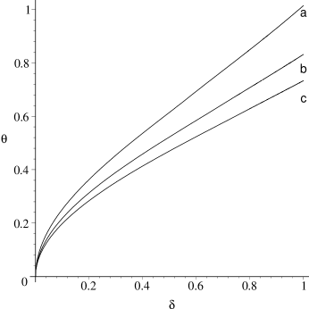
Figure 5: Bending angle as a function of the time parameter $\delta$. The three graphs show the bending angle for the same initial radius $R_{0}=9M$ for 3 different values of $R_{e}$: (a) $5.5M$, (b) $6.5M$, and (c) $7.5M$.

The frequency observed at infinity is different from the frequency at emission because of two reasons: (1) Difference of the gravitational potential at the point of emission and observation, (gravitational redshift), and (2) The velocity of the emitting surface (Doppler shift). The photons emitted from the surface of $R_{e}$ experience the same gravitational redshift independent of their angular positions (bending angle) of emission. However Doppler shift depends on the relative velocity of the surface of emission with respect to the distant observer, and hence it depends on the bending angle (or the impact parameter $l$). The corresponding total frequency shift can be calculated from eq.(23). Since the arrival time depends on the impact parameter as well, the frequency shift then can be plotted as a function of the arrival time. The calculated ratio of emitted frequency to the observed one, $\Phi$, for a short flash as a function of the time parameter $\delta$ is shown in Fig. 6. Three curves which meet one another at $\delta=1$ correspond to the three cases IIa,b,c. The forth curve corresponds to the case I.

Figure 6: Redshift factor for a freely collapsing surface as a function of the time parameter $\delta$ for the cases I, and IIa,b,c.

It is interesting that the redshift due to the gravity is substantially cancelled by the Doppler shift for the tangentially emitted light. Really, using (19) and (23) we obtain for the redshift factor $\Phi$ the following expression

$$\Phi_{T}={\sqrt{1-v_{i}^{2}\over f(R_{e})}}\,.$$ (87)

For a free fall from the radius $R_{0}$ one has

$$1-v_{i}^{2}={1-2M/R\over 1-2M/R_{0}}\,.$$ (88)

Thus

$$\Phi_{T}=\frac{1}{\sqrt{1-2M/R_{0}}}\,.$$ (89)

It means that for the “last rays” (that is for rays with $l=l_{T}$), the redshift depends only on the initial radius $R_{0}$ and does not depend on the radius of emission $R_{e}$. For this reason the three curves IIa,b,c in Fig. 6 merge at the same value $3/\sqrt{7}\approx 1.134$ at $\delta=1$ (that is for $l=l_{T}$). Relation (89) also shows that for $R_{0}=\infty$ the gravitational redshift is exactly cancelled by the Doppler shift jaffe .

Since for direct radial rays ($l=0$) both effects “work” in the same direction, one can expect that for a given $R_{0}$ the redshift will be larger for smaller values of $R_{e}$. The Fig. 6 clearly demonstrates this.

V.3 Light curves

Let us discuss now normalized flux as a function of the time parameter $\delta$. We call the corresponding graph a light curve. In case I ($R_{0}=5M$, $R_{e}=4.8M$), the light curves for a short flash from the collapsing spherical surface are shown Fig.(7). The plot IA is a light curve for ${\bf I}=1$ and the plot IB is a light curve for ${\bf I}=\cos\beta(l)$ (Lambert’s law). Similar light curves for a static spherical surface are shown for comparison at Fig. 8.

Figure 7: Light curves for ${\bf I}=1$ (IA) and ${\bf I}=\cos\beta(l)$ (IB) for a freely-collapsing surface with $R_{e}/M=4.8$ and $R_{0}/M=5.4M$.

Figure 8: Light curves for ${\bf I}=1$ (IA) and ${\bf I}=\cos\beta(l)$ (IB) for a static surface with $R_{e}/M=4.8$.

For the case II ($R_{0}=9M$) the light curves for A and B type of the radiating surface are shown in Fig. 9 and Fig. 10, respectively. Each of the figures contains 3 curves corresponding to IIa,b,c cases.

Figure 9: Light curves for ${\bf I}=1$ for the cases IIa,b,c.

Figure 10: Light curves for ${\bf I}=\cos\beta(l)$ for the cases IIa,b,c.

Let us discuss now qualitative behavior of the light curves. The observed normalized flux ${\bf F}(t)$ given by eq. (82) is a product of 3 factors: (1) a kinematic term $W_{e}(t)/W_{0}$, (2) a redshift factor $(\Phi_{e}(t)/\Phi_{0})^{-4}$, and (3) a normalized intensity of the emission ${\bf I}$. The third factor depends on the model of the radiating surface and it does not depend on the arrival time. The first two factors are time dependent. The arrival time dependence of $W_{e}$ is essentially determined by the factor of $|Z-\sigma v_{i}|$ in eq.(72), which is a decreasing function of $\delta$ and vanishes for $\delta=1$. Hence every light curves should cross the zero-flux axis at $\delta=1$. For a static surface $v_{i}=0$ and $Z$ (and hence $W_{e}(t)$) vanishes at $\delta=1$, where $l=l_{max}$. For a collapsing surface $v_{i}<0$ and the observable flux vanishes not for $l_{max}$ (where $Z=0$) but for the backward emission with $l=l_{T}$. Hence one can expect longer duration of observed flux for the emission from a collapsing surface compared to the emission from a static surface. The effect of motion of the collapsing surface becomes stronger for larger $v_{i}$. For example for a given $R_{0}=9M$, $\Delta t_{max}$ is calculated to be larger for smaller $R_{e}$ for which $v_{i}$ is larger (see Table).

The redshift factor $\Phi$ depends basically on the relative receding velocity of the emitting region (determined by the bending angle) with respect to the distant observer. The relative receding velocity is decreasing as the bending angle is increasing. Since the arrival time difference becomes larger for a ray with larger bending angle, one can expect the enhancement of a factor, $\Phi^{-4}$, for larger $\delta$. The main effect of the frequency shift for the observed flux due to the collapsing surface is the enhancement of the flux for lately arriving rays. As a result the shape of the light curve for a collapsing surface is changing from that of a static surface in such way that the flux decreasing in $\delta$ is delayed and the sharp forward peak at $\delta=0$ becomes a rather smooth peak as shown in Fig. (7). For sufficiently large collapsing velocity, for example for $R_{0}=9M$ and $R_{e}=5.5M$, one can observe that position of the peak in the light curve also changes from $\delta=0$ to a later arrival time $\delta\neq 0$ for the isotropic intensity profile(A) as shown at Fig. (9). The emission angle with respect to the normal to the surface, $\beta$, varies from 0 to $\pi/2$ as the impact parameter $l$ varies from 0 to $l_{max}$ and further to $l_{T}$. Hence the intensity profile of (B) with $I^{(e)}=b\cos(\beta(l))$ suppresses the enhancement due to the factor $\Phi^{-4}$ for lately arriving rays substantially as shown in Fig. 10. The light curves from the static surface for intensity profile (A) and (B) are also shown in Fig. 8 for comparison.

VI Discussion

In this work, we discussed characteristics of the radiation emitted from a surface of a collapsing object. We studied a simplified (toy) model in which a radiation of massless particles has a sharp in time pulse profile and it happens at the surface at the same instant of time (from a point of view of a comoving observer). In this approximation both integrals over the time and frequency which enter a general expression for the observed flux can be taken. As a result we obtained an expression for the normalized flux as a function of the time of the observation. We demonstrated that for a short in time flash, the observed normalized flux can be expressed as a product of three terms: a kinetic term ($W$), a redshift factor ($\Phi$), and the intensity of the emitted radiation. The intensity of the emitted radiation is model dependent. In particular it depends on the model of the radiating surface region. The other two factors are universal and depend only on the equation of motion of the collapsing surface. The dependence of $W$ and $\Phi$ on the arrival time is quite different. We assume that the collapse starts at some radius $R_{0}$ and the emission occurs at the radius $R_{e}$. Under this assumption all the characteristics of the radiation such as its duration, redshift, and the form of the light curves (for chosen intensity of emission) depend only on these 2 parameters. To obtain the light curves one needs to integrate the equations for the light propagation in the Schwarzschild metric. The corresponding integration can be performed in terms of elliptic integrals. But the calculation of the flux requires solving an inexplicit equation which contains the elliptic integrals.

In order to solve this problem we developed an analytical approximation for the bending angle and time delay for null rays emitted by a collapsing surface. In the case of the bending angle this approximation is an improved version of the earlier proposed BL-approximation ll ; bel . For rays emitted at $R>2R_{g}$ the accuracy of the approximation for the bending angle and time delay proposed in the present paper is of order (or less) than 2-3$\%$. By using this approximation we obtained an explicit formula for the observed normalized flux, which not only allows one very efficient numerical calculations of the characteristics of the radiation, but also appears to be useful for understanding the qualitative features of the radiation.

Even for a static object the effects of the General Relativity allows one to ”see” a part of its opposite side surface. For a collapsing object this effect is more profound. As a result, the duration of the flux is elongated. Another difference is that the sharp decrease in time for the static surface is delayed and ”smoothed out” so that the peak becomes broader. For a sufficiently large collapsing velocity the peak position can even be shifted to $\delta>0$. We demonstrated these features by considering two examples of collapses starting at $R_{0}=5.4M$ and $R_{0}=9M$.

Though in this paper we focused on a model of brief in time flash emission, some of its results (improved analytic approximation) might be of the interest for other astrophysically interesting problems.

Appendix A Calculation of ${dl}/{d\tau}$

Let us fix $\tau_{e}$ in (31) and consider time delay $\Delta_{+}(l;\tau,\tau_{e})$ as a function of $l$ and $\tau$. Consider a rays which reach the observer at the same time $t$. For these rays $\Delta_{+}(l;\tau,\tau_{e})$ is the same. This establish the relation between $l$ and $\tau$: $l=l_{t}(\tau)$. To obtain this expression we differentiate (31) with respect to $\tau$, keeping $t$ fixed.

For a forward ray one has

$$\dot{t}^{(e)}-{\dot{R}\over fZ}+{\partial T\over\partial l}\dot{l}=0\,.$$ (90)

We denote by a dot the derivative $d/d\tau$. Using (9) we get

$$\dot{l}=-{(Z-v_{i})\dot{t}^{(e)}\over Z(\partial T/\partial l)}\,.$$ (91)

To calculate the partial derivative

$${\partial T\over\partial l}={\partial T\over\partial{\cal Z}}{\partial{\cal Z}\over\partial l}$$ (92)

we use the approximate expression (61). We have

$${\partial T\over\partial{\cal Z}}=R+MQ^{\prime}\,,$$ (93)

$${\partial{\cal Z}\over\partial l}={l\over R^{2}Z}\,.$$ (94)

Combining these results we obtain

$$W_{+}=l|\dot{l}|={R(Z-v_{i})\dot{t}^{(e)}\over{\cal J}_{+}}\,.$$ (95)

where

$${\cal J}_{+}=1+(M/R)Q^{\prime}\,.$$ (96)

For backward rays the calculation of $\dot{l}$ is similar. Using the equation (33) for rays reaching the observer at the same time $t$ one obtains the following equation for $l_{t}(\tau)$

$$\dot{t}^{(e)}+{\dot{R}\over f(R)Z(l,R)}-{\partial T\over\partial l}\dot{l}+2\left[\dot{T}(r_{t})-{\dot{r}_{t}\over f(r_{t})}\right]=0\,.$$ (97)

Using (26) we find

$$\dot{r}_{t}={l\dot{l}f^{2}(r_{t})\over(r_{t}-3M)}\,.$$ (98)

We also have

$$Z(r_{t})=0\,,\hskip 14.22636pt{\cal Z}(r_{t})=1/f(r_{t})\,.$$ (99)

Using the approximate expression for $T$, (61), we have

$$T_{,r_{t}}={\cal Z}(r_{t})+[r_{t}+MQ^{\prime}_{r_{t}}]{d{\cal Z}\over dr_{t}}\,.$$ (100)

Here $Q^{\prime}_{r_{t}}=Q^{\prime}(f^{-1}(r_{t}))$. Using these relation we obtain

$$\dot{T}(r_{t})-{\dot{r}_{t}\over f(r_{t})}=-l\dot{l}{2M\over r_{t}^{2}(r_{t}-3M)}[r_{t}+MQ^{\prime}_{r_{t}}]\,.$$ (101)

This allow us to rewrite (97) in the form

$$\dot{t}^{(e)}(Z+v_{i})R=l\dot{l}\left[{\cal J}_{+}+{4MRZ\over r_{t}^{2}}{r_{t}+MQ^{\prime}_{r_{t}}\over r_{t}-3M}\right]\,.$$ (102)

Finally we obtain

$$W_{-}=l|\dot{l}|={R(Z+v_{i})\dot{t}^{(e)}\over{\cal J}_{-}}\,,$$ (103)

$${\cal J}_{-}={\cal J}_{+}+{4MRZ\over r_{t}^{2}}{r_{t}+MQ^{\prime}_{r_{t}}\over r_{t}-3M}\,.$$ (104)

References

- (1) J.M. Lattimer and M. Prakash, Science 304, 536(2004)
- (2) K.R. Pechenick, C.Ftaclas and J.M. Cohen, Astrophys. J. 274, 846(1983)
- (3) D.A. Leahy and L. Li, MNRAS 277, 1177(1995)
- (4) A. Beloborodov, Astrophys. J. 566, L85(2002)
- (5) P. Meszaros and H. Riffert, Astrophys. J. 327, 712(1988); H. Riffert and P. Meszaros , Astrophys. J. 325, 207(1988)
- (6) C.Cadeau, D.A. Leahy and S. M. Morsink, Astrophys. J. 618, 451(2005)
- (7) W.L. Ames and K.Thorne, Astrophys. J. 151, 659(1968)
- (8) J. Jaffe, Ann. Phys.(N.Y.) 55, 374(1969)
- (9) K. Lake and R.C. Roeder, Astrophys. J. 232, 277(1979)
- (10) G.E. Brown and H. Bethe, Astrophys. J. 423, 659(1994)
- (11) S. Shapiro, Astrophys. J. 472, 308(1996)
- (12) T.W. Baumgarte, H-T Janka, W. Keil, S.L. Shapiro and S.A. Teukolsky, Astrophys. J. 468, 823(1996)
- (13) T. Schaefer, hep-ph/0304281
- (14) C. Vogt, R. Rapp and R. Ouyed, Nucl. Phys. A. 735, 543(2004)
- (15) R.C. Tolmann, Pro. Nat. Acad. Sci. U.S.A. 20, 169(1934)
- (16) R. Oppenheimer and H. Snyder, Phys. Rev. 56, 455(1939)
-
(17)
In the presence of both, forward and backward rays,
the integral over the impact parameter is understood as a sum
of two integrals, one over for the forward
radiation and another over for the backward
radiation. Thus the integral (68) stands for
We shall use this convension for the other similar integrals.(105) - (18) C.W. Misner, K. S. Thorne, J. A. Wheeler, Gravitation(W. H. Freman and Co., San Francisco, 1972)
- (19) M.A. Podurets, Sov. Astron. 8, 868(1965)
- (20) See for example, E. Bohm-Vitense, Introduction to Stellar Astrophysics(Cambridge University Press, Cambgridge, England, 1989).
- (21) J.M. Lattimer and M. Prakash, Astrophys. J. 550, 426(2001)