On characteristic initial data for a star orbiting a black hole

Abstract

We take further steps in the development of the characteristic approach to enable handling the physical problem of a compact self-gravitating object, such as a neutron star, in close orbit around a black hole. We examine different options for setting the initial data for this problem and, in order to shed light on their physical relevance, we carry out short time evolution of this data. To this end we express the matter part of the characteristic gravity code so that the hydrodynamics are in conservation form. The resulting gravity plus matter relativity code provides a starting point for more refined future efforts at longer term evolution. In the present work we find that, independently of the details of the initial gravitational data, the system quickly flushes out spurious gravitational radiation and relaxes to a quasi-equilibrium state with an approximate helical symmetry corresponding to the circular orbit of the star.

I Introduction

The problem of computing the evolution of a self-gravitating object, such as a neutron star, in close orbit about a black hole is of clear astrophysical importance, both to understand systems thought to drive such spectacular phenomena as gamma-ray bursts (see, for instance, rees ) and to predict the details of the gravitational radiation which could be observed by the new generation of gravitational wave detectors (see, for instance, ct ). Furthermore, the dynamics of the system could be quite rich. For instance, the tidal interaction between the black hole and the star could be strong enough to tidally disrupt the star with a consequent drastic change in the emitted waves vallisneri . Alternatively, as has recently been suggested davies , only a portion of the star’s mass might be transferred to the black hole and angular momentum transfer might boost what remains of the star into a wider orbit. The system would then undergo another inspiral phase and this process might repeat itself. Consequently, the expected gravitational waves would display a very rich structure of several ‘chirp-phases’.

A better understanding of these possibilities requires, as basic building blocks, solving Einstein equations coupled to an appropriate matter field without restrictive assumptions. To this end, long-term well behaved numerical simulations must be available. Presently, several numerical relativity codes for treating the two body problem are either being developed or planned baumgarte ; shibata ; miller ; hawke , as the know-how for simulating Einstein equations becomes more mature. Although most of these efforts concentrate on the Cauchy approach to Einstein equations, there are alternatives approaches which have been successful for specific problems. In particular, the characteristic formulation of general relativity has shown remarkable robustness to deal with single black hole space-times. Stable axisymmetric studies of Einstein equations coupled to perfect fluids have been achieved siebel2 ; siebel1 ; and our previous work has produced stable three-dimensional characteristic numerical relativity codes for vacuum space-times hpn and for fluid space-times with very small pressure mat .

This paper develops further methodology necessary for the evolution of a self-gravitating star or other object in orbit near a Schwarzschild black hole. Towards this final goal, we examine the issue of setting initial data. In either the characteristic or Cauchy approaches to this problem, a serious source of physical ambiguity is the presence of spurious gravitational radiation in the initial gravitational data. Because the characteristic approach is based upon a retarded time foliation, the resulting spurious outgoing waves can be computed by carrying out a short time evolution. We carry out such a study in the present work. We find that, independently of the details of the initial gravitational data, such spurious waves quickly radiate away, and that the system relaxes to a quasi-equilibrium state with an approximate helical symmetry corresponding to the circular orbit of the star. This result provides important physical justification of recent approaches for initializing the Cauchy problem which are based on imposing an initial helical symmetry klein ; shibatafriedman ; yocook ; grandclement ; andrade .

We also examine two useful tools which can be applied to long term simulations as well as to the initial data problem: (i) a tool to monitor the development of a singularity in the null coordinates and (ii) a tool to use co-rotating coordinates so that an orbiting star remains approximately at a fixed coordinate position.

A crucial ingredient of any hydrodynamical simulation is the proper handling of shocks and discontinuities and the proper conservation of baryonic mass. Robust numerical techniques are available to this end, which express the system in a conservation form designed for handling discontinuities in the fluid leveque . In particular, high resolution shock capturing schemes utilize the fluid’s characteristic propagation speeds to capture the discontinuities in an accurate way. In the present work, we follow the formalism presented in philiptoni , where the general relativistic hydrodynamic equations are presented in a conservation form adapted to both the Cauchy and the characteristic formulations. High resolution shock capturing schemes have been successfully incorporated in the characteristic approach in the case of axisymmetric space times siebel2 ; siebel1 . Although this is the ideal approach to the hydrodynamic problem, here we implement a less time consuming algorithm due to Davis davis . This approach has limitations in dealing with shock formation but is sufficient for our present purpose to study the initial data problem.

The initial data problem for the characteristic formulation of relativity hpn has received little attention in comparison with that for the Cauchy problem. This is partly because the data for the characteristic formulation is unconstrained, whereas the data for the Cauchy formulation has to satisfy an elliptic system of constraints. Even so, in both formulations, care must be taken to set matter data that represents the intended physical problem. In particular, it is not trivial to set gravitational data free of spurious gravitational radiation. A method for initializing characteristic data based upon a correspondence with Newtonian theory newt1 ; newt2 guarantees that the resulting gravitational radiation obeys the Einstein quadrupole formula in the Newtonian regime iww ; qf . However, as discussed in newt1 , the domain of applicability of the method is limited to when (i) the Newtonian potential $\Phi$ of the star satisfies $\Phi\ll 1$ and (ii) relative velocities are much slower than the speed of light. The second issue could be easily dealt with by making the orbital radius $a$ of the star large compared to the black hole mass $M$. However, the following practical reasons make it desirable to initialize the star in a close orbit with $a\leq 10M$ (for which $v\geq c/3$):

• Since the orbital period of the star around the black hole scales as $a^{3/2}$, a simulation starting from large $a$ would require very time consuming runs in a regime that could be described approximately by less expensive perturbative treatments.

• When using spherical coordinates, the resolution at large $a$ worsens when using a uniform grid. Computer resources limit the number of angular grid points that can be used. Thus, adequate resolution of the star requires that $a$ be small.

• The most interesting physics, intractable by other means, occurs when the compact object is at small $a$.

Construction of mathematically consistent initial data is much simpler than construction of physically meaningful data. While the former involves the solution of constraint equations (if any), the latter is less mathematically explicit. Not only does one want matter data describing an orbiting star but also gravitational data with minimal spurious radiation. Success must be gauged through actual evolution of the data and analysis of the resulting space-time.

There are basically no constraint equations for the gravitational initial data in the characteristic formulation so that mathematically consistent data is trivial to prescribe. In order to investigate the physical problem we proceed by investigating gravitational data based upon two completely different underlying assumptions:

• Gravitational initial data obtained by means of the Newtonian correspondence method

• Spherically symmetric gravitational data corresponding to a shear-free initial null hypersurface.

The first method applies only to a quasi-Newtonian regime. The second method ignores the focusing effect of the star which introduces shear in its nearby null rays. Nevertheless, in both cases the gravitational field relaxes to a state of approximate helical symmetry after about a light-crossing time for the system. These results support the view that the details of the initial gravitational data may not be important as long as they are reasonable and some time is evolved in which the spurious radiation flushes out.

The plan of the paper is as follows: in Sec. II with present a summary of previous work on the characteristic formulation of numerical relativity and on conservative hydrodynamics. The construction of initial matter and gravitational data is covered in Sec III in both stationary and co-rotating frames. In Sec. IV we discuss the conditions under which coordinate singularities might develop. Some details of the numerical implementation are presented in Sec. V. Computational tests and results are given in Sec. VI.

II Summary of previous results and notation

II.1 Characteristic formulation of Einstein equations

The formalism for the numerical evolution of Einstein’s equations, in null cone coordinates, is well known rai83 ; hpn ; cce (see also ntb93 ; ntb90 ; rai83 ), and is based upon the analytic treatments of bondi ; sachs ; tam . For the sake of completeness, we give here a summary of the formalism, including some of the necessary equations. The version of the gravity code being used here is fully described in roberto ; particle . It has most recently been applied in modemode .

We use coordinates based upon a family of outgoing null hypersurfaces. We let $u$ label these hypersurfaces, $x^{A}$ $(A=2,3)$, label the null rays and $r$ be a surface area coordinate. In the resulting $x^{\alpha}=(u,r,x^{A})$ coordinates, the metric takes the Bondi-Sachs form bondi ; sachs

$$ds^{2} = -\left(e^{2\beta}(1+{W\over r})-r^{2}h_{AB}U^{A}U^{B}\right)du^{2}-2e^{2\beta}dudr-2r^{2}h_{AB}U^{B}dudx^{A}$$ (1)

$$+ r^{2}h_{AB}dx^{A}dx^{B},$$

where $h^{AB}h_{BC}=\delta^{A}_{C}$ and $det(h_{AB})=det(q_{AB})$, with $q_{AB}$ a unit sphere metric. We work in stereographic coordinates $x^{A}=(q,p)$ for which the unit sphere metric is

$$q_{AB}dx^{A}dx^{B}=\frac{4}{F^{2}}(dq^{2}+dp^{2}),\mbox{ where }F=1+q^{2}+p^{2}.$$ (2)

Our previous work used $P=1+q^{2}+p^{2}$, here we change notation to $F$ because we will use $P$ to represent pressure. We also introduce a complex dyad $q^{A}=\frac{F}{2}(1,i)$ with $i=\sqrt{-1}$. For an arbitrary Bondi-Sachs metric, $h_{AB}$ can then be represented by its dyad component

$$J=h_{AB}q^{A}q^{B}/2,$$ (3)

with the spherically symmetric case characterized by $J=0$. We introduce the (complex differential) eth operators $\eth$ and $\bar{\eth}$  eth , as well as a number of auxiliary variables $K=h_{AB}q^{A}\bar{q}^{B}/2$, $U=U^{A}q_{A}$, $Q_{A}=r^{2}e^{-2\,\beta}h_{AB}U^{B}_{,r}$, $Q=Q_{A}q^{A}$, $B=\eth\beta$, $\nu=\bar{\eth}J$ and $k=\eth K$.

The Einstein equations $G_{ab}=0$ decompose into hypersurface equations, evolution equations and conservation laws. Here we note that the hypersurface equations form a hierarchical set for $\nu_{,r}$, $k_{,r}$, $\beta_{,r}$, $B_{,r}$, $Q_{,r}$, $U_{,r}$ and $W_{,r}$, and the evolution equation is an expression for $(rJ)_{,ur}$. The explicit form of the equations is given in roberto in the vacuum case and in mat for the matter terms. Note the following correction to the matter source term in Eq. mat –(31)

$$2\left(rJ\right)_{,ur}-\left((1+r^{-1}W)\left(rJ\right)_{,r}\right)_{,r}=-r^{-1}\left(r^{2}\eth U\right)_{,r}+2r^{-1}e^{\beta}\eth^{2}e^{\beta}-\left(r^{-1}W\right)_{,r}J+N_{J}$$

$$+\frac{4e^{2\beta}\pi(\rho+P)}{r}\left((J\bar{V}_{ang}-KV_{ang})^{2}+V^{2}_{ang}\right),$$ (4)

where $V_{ang}=v_{A}q^{A}$ mat (with $v_{\alpha}$ the velocity) and $N_{J}$ are defined in hpn and roberto . The remaining Einstein equations are the conservation conditions which are satisfied here because of the simple choice of boundary data.

The null cone problem is normally formulated in the region of space-time between a timelike or null worldtube $\Gamma$ and ${\cal I}^{+}$. We represent ${\cal I}^{+}$ on a finite grid by using a compactified radial coordinate $x=r/(1+r)$. The numerical grid is regular in $(x,q,p)$, and consists of two stereographic patches covering the north and south hemispheres, each containing $n_{x}\times n_{q}\times n_{p}$ grid points. The $x-$grid covers the range $[0.5,1]$, and each angular grid patch extends at least two grid points beyond the equator so that there is an overlap region.

The mass of the Schwarzschild black hole is denoted as $M$, and in all the computational tests we will take $M=1$. The star has mass $m$ and radius $R_{*}$.

II.2 Characteristic hydrodynamics in conservation form

The integration of the hydrodynamical equations is done in a more accurate way if the system can be expressed in conservation form. This allows for better conservation of baryonic mass and the possibility of exploiting the characteristic structure of the equations to resolve shocks via Godunov methods leveque . Here we use the formalism developed in  philiptoni , where the equations $\nabla_{a}J^{a}=0$, $\nabla_{a}T^{ab}=$ are expressed in conservation form as,

$$\partial_{x^{0}}(\sqrt{-g}{\bf U}^{A})+\partial_{x^{j}}(\sqrt{-g}{\bf F}^{jA})={\bf S}^{A}\,,$$ (5)

where $U^{A}=(D,S^{i},E)$ are “conservative” variables defined as,

$$D = {\bf U}^{0}=J^{0}=\rho u^{0}\,,$$ (6)

$$S^{i} = {\bf U}^{i}=T^{0i}=\rho hu^{0}u^{i}+Pg^{0i}\,,$$ (7)

$$E = {\bf U}^{4}=T^{00}=\rho hu^{0}u^{0}+Pg^{00}\,.$$ (8)

and the fluxes and sources are

$${\bf F}^{j0} = J^{j}=\rho u^{j}\,,$$

$${\bf F}^{ji} = T^{ji}=\rho hu^{i}u^{j}+Pg^{ij}\,,$$

$${\bf F}^{j4} = T^{j0}=\rho hu^{0}u^{j}+Pg^{0j}\,,$$ (9)

$${\bf S}^{0} = 0\,,$$

$${\bf S}^{i} = -\sqrt{-g}\,\Gamma^{i}_{\mu\lambda}T^{\mu\lambda}\,,$$

$${\bf S}^{4} = -\sqrt{-g}\,\Gamma^{0}_{\mu\lambda}T^{\mu\lambda}\,.$$ (10)

The state of the system is uniquely described in terms of the geometry, the primitive matter variables $(\rho,P,h,u^{a})$ or the conservative variables, the fluid’s equation of state and the normalization condition $u^{a}u_{a}=-1$. In the particular case of a perfect fluid which we consider here, the relation between primitive and conservative variables is straightforward and does not require expensive inversion methods (see philiptoni for details).

III Initial and boundary data

There exist only rough physical guidelines for prescribing initial matter and gravitational field data in general relativity for a star orbiting a black hole. Here we present initial data which is at least mathematically consistent with Einstein’s equations and has some underlying connection with the Newtonian picture of a star in equilibrium, which is orbiting a collapsing central object. The Newtonian picture is not a good approximation to the relativistic regime in which we run our simulations. Nevertheless, the justification for this approach is that the evolutions, presented in Sec. VI, relax on the order of a light crossing time to a more astrophysically realistic state, as extraneous gravitational wave content in the initial data is radiated away, and the gravitational field adapts to the approximate symmetry of the matter distribution. This relaxed state is remarkably independent of the initial gravitational data.

III.1 The initial matter data

We prescribe the initial matter data within a simple Newtonian framework. We take the star to be a spherically symmetric polytrope of index $n=1$ chandra1 with

$$\rho=\frac{m\sin{\frac{R\pi}{R_{*}}}}{4RR_{*}^{2}}$$ (11)

for $R\leq R_{*}$, and $\rho=0$ for $R>R_{*}$, where $\rho$ is the density at radius $R$. Denoting the pressure by $P$, the equation of state is

$$P=\frac{2R_{*}^{2}\rho^{2}}{\pi}.$$ (12)

Note that the maximum value of $P/\rho$ is $m/2R_{*}$, so that Newtonian theory gives a good approximation to an equilibrium configuration provided the polytrope is not near its Schwarzschild radius. We prescribe the initial matter velocity to be uniform across the polytrope. In the evolutions considered later the center of the polytrope will be placed at $(q=p=0,r=a)$, with the velocity set for a circular orbit, so that $V^{r}=V^{p}=0$ initially.

The assumption that the polytrope is spherically symmetric is always valid mathematically since the initial data is freely specifiable, but the star remains in equilibrium only if there is no tidal force. Of course, it is known how to compute the tidal distortion of a polytrope in equilibrium within both Newtonian gravity and post-Newtonian general relativity – see for example uryu ; lom . However, in the simulations of a star orbiting a black hole presented in this paper, the polytrope is not stable against tidal disruption, i.e. the simple Roche indicator $\epsilon_{R}\equiv R_{*}/a\sqrt[3]{2M/m}\gg 1$. Thus, for the present work, there is no point in calculating an equilibrium configuration for the tidal distortion.

In order to obtain physical characteristic initial data for the problem we transform the above Newtonian initial data into density, velocity and gravitational fields within the framework of a Bondi-Sachs metric in general relativity. As discussed in Sec. I, this needs to be done in a relativistic regime in which the Newtonian correspondence method newt1 ; newt2 ; iww is only roughly approximate.

The density and velocity matter fields are regarded as being given in a Lorentzian frame in the Minkowski space-time in which the center of mass of the polytrope is at rest. Then a coordinate transformation is made from this local Lorentz frame to the global Bondi-Sachs coordinates. This approach is strictly valid only if space-time curvature can be neglected in the vicinity of the star, which requires that the radius of the star must be small and that its gravitational source effect must be negligible. The approach has a proper Newtonian correspondence in the limiting case of small velocities, small $m/R_{*}$ and large $a$.

III.1.1 The density and velocity fields

We prescribe initial data ($\rho$, $V^{\alpha}$) for the localized distribution of matter described in Sec. III.1. The matter is described in a (locally) inertial frame $S_{I}=(t,x,y,z)$ in which the center of mass of the matter is instantaneously at rest at the origin. Globally, we have Bondi-Sachs coordinates centered about the black hole (with mass $M$). To the extent that the gravitational effect of the matter can be neglected, the geometry is spherically symmetric and can be described in Eddington-Finkelstein coordinates $S_{E}=(u,r,q,p)$. The origin of $S_{I}$ is at $u=0,r=a,q=p=0$ and, for simplicity, we choose a central matter velocity of the form $(V^{u},0,V^{q},0)$ in $S_{E}$. Except in the case $M=0$, the curvatures of $S_{I}$ and $S_{E}$ are different, and thus it is not possible to construct a unique global transformation between $S_{I}$ and $S_{E}$. However, we can construct a transformation that is valid near the origin of $S_{I}$.

We proceed by constructing a locally inertial frame $S^{\prime}=(t^{\prime},x^{\prime},y^{\prime},z^{\prime})$ whose origin is at $O=(u=0,r=a,q=0,p=0)$ and with the $S^{\prime}$ axes pointing in the $(u,r,q,p)$ directions. In general, $S_{I}$ is moving relative to $S^{\prime}$. When the black hole mass $M=0$, the space-time is flat and there is an unambiguous transformation from $S^{\prime}$ to $S_{E}$

$$t^{\prime} = u+(r-a)$$

$$x^{\prime} = \frac{2rq}{1+q^{2}+p^{2}}$$

$$y^{\prime} = \frac{2rp}{1+q^{2}+p^{2}}$$

$$z^{\prime} = \frac{2r}{1+q^{2}+p^{2}}-r-a.$$ (13)

When $M\neq 0$, the metric is Schwarzschild in the Eddington-Finkelstein form

$$ds^{2}=-\Big{(}1-\frac{2M}{r}\Big{)}du^{2}-2du\;dr+\frac{4r^{2}}{(1+q^{2}+p^{2})^{2}}(dq^{2}+dp^{2}).$$ (14)

An orthonormal tetrad aligned with $S^{\prime}$ and defined in $S_{E}$ at the point $O$ is given by

$$X_{(t)}^{a} = (\Big{(}1-\frac{2M}{a}\Big{)}^{-\frac{1}{2}},0,0,0)$$

$$X_{(x)}^{a} = (0,0,\frac{1}{2a},0)$$

$$X_{(y)}^{a} = (0,0,0,\frac{1}{2a})$$

$$X_{(z)}^{a} = (-\Big{(}1-\frac{2M}{a}\Big{)}^{-\frac{1}{2}},\Big{(}1-\frac{2M}{a}\Big{)}^{\frac{1}{2}},0,0).$$ (15)

In a neighborhood of $O$, $S_{E}$ and $S^{\prime}$ are related by the transformation

$$u = \Big{(}1-\frac{2M}{a}\Big{)}^{-\frac{1}{2}}t^{\prime}-\Big{(}1-\frac{2M}{a}\Big{)}^{-\frac{1}{2}}z^{\prime}$$

$$r-a = \Big{(}1-\frac{2M}{a}\Big{)}^{\frac{1}{2}}z^{\prime}$$

$$q = \frac{x^{\prime}}{2a}$$

$$p = \frac{y^{\prime}}{2a},$$ (16)

from which we construct the inverse transformation

$$t^{\prime} = \Big{(}1-\frac{2M}{a}\Big{)}^{\frac{1}{2}}u+\Big{(}1-\frac{2M}{a}\Big{)}^{-\frac{1}{2}}(r-a)$$

$$x^{\prime} = 2aq$$

$$y^{\prime} = 2ap$$

$$z^{\prime} = \Big{(}1-\frac{2M}{a}\Big{)}^{-\frac{1}{2}}(r-a).$$ (17)

In the $M=0$ case, the transformation is unambiguous and global, but when $M\neq 0$ the transformation to a locally inertial system can only be defined in a neighborhood of $O$. Nevertheless we need a transformation that is valid in a region around $O$, which we construct by combining (13) and (17) to obtain

$$t^{\prime} = \Big{(}1-\frac{2M}{r}\Big{)}^{\frac{1}{2}}u+\Big{(}1-\frac{2M}{r}\Big{)}^{-\frac{1}{2}}(r-a)$$

$$x^{\prime} = \frac{2rq}{1+q^{2}+p^{2}}$$

$$y^{\prime} = \frac{2rp}{1+q^{2}+p^{2}}$$

$$z^{\prime} = \Big{(}\frac{2r}{1+q^{2}+p^{2}}-r-a\Big{)}\Big{(}1-\frac{2M}{r}\Big{)}^{-\frac{1}{2}}.$$ (18)

The transformation (18) reduces to (13) when $M=0$, and to (17) near the point $O$.

It is most convenient to describe the matter in an inertial frame in which it is at rest which, in general, is not the case for $S^{\prime}$. In order to achieve this we need to make a Lorentz transformation to coordinates $S_{I}=(t,x,y,z)$. In the case that the matter velocity is entirely in the $q$-direction, which includes the case of a quasi-circular orbit around the black hole, the transformation between $S_{E}$ and $S_{I}$ is

$$t=\gamma(t^{\prime}-vx^{\prime}),\;\;x=\gamma(x^{\prime}-vt^{\prime}),\;\;y=y^{\prime},\;\;z=z^{\prime},$$ (19)

where $v$ is the velocity between $S_{I}$ and $S^{\prime}$, and $\gamma$ is the usual Lorentz factor, $\gamma=(1-v^{2})^{-\frac{1}{2}}$. Then combining (19) and (17) we find

$$t = \gamma\Bigg{(}\Big{(}1-\frac{2M}{r}\Big{)}^{\frac{1}{2}}u+\Big{(}1-\frac{2M}{r}\Big{)}^{-\frac{1}{2}}(r-a)-\frac{2rqv}{1+q^{2}+p^{2}}\Bigg{)}$$

$$x = \gamma\Bigg{(}\frac{2rq}{1+q^{2}+p^{2}}-v\Big{(}1-\frac{2M}{r}\Big{)}^{\frac{1}{2}}u-v\Big{(}1-\frac{2M}{r}\Big{)}^{-\frac{1}{2}}(r-a)\Bigg{)}$$

$$y = \frac{2rp}{1+q^{2}+p^{2}}$$

$$z = \Big{(}\frac{2r}{1+q^{2}+p^{2}}-r-a\Big{)}\Big{(}1-\frac{2M}{r}\Big{)}^{-\frac{1}{2}}.$$ (20)

The transformation (20) is sufficient for setting scalar initial matter data, such as the density. Given an $S_{E}$ grid at $u=0$, we find for each point the coordinates $(x,y,z)$. The density is then determined by its values in $S_{I}$. We also need to set the initial 4-velocity. In $S_{I}$ the 4-velocity is $V^{(I)}_{a}=(-1,0,0,0)$. Thus in $S_{E}$ the covariant 4-velocity is

$$V^{(E)}_{a} = \frac{\partial x^{(I)b}}{\partial x^{(E)a}}V^{(I)}_{b}=-\frac{\partial t}{\partial x^{(E)a}}$$ (21)

$$= \gamma\bigg{(}-\Big{(}1-\frac{2M}{r}\Big{)}^{\frac{1}{2}},$$

$$\frac{2qv}{1+q^{2}+p^{2}}-\Big{(}1-\frac{2M}{r}\Big{)}^{-\frac{1}{2}}+\frac{(r-a)M}{r^{2}}\Big{(}1-\frac{2M}{r}\Big{)}^{-\frac{3}{2}},$$

$$\frac{2rv(1+p^{2}-q^{2})}{(1+q^{2}+p^{2})^{2}},$$

$$-\frac{4vqpr}{(1+q^{2}+p^{2})^{2}}\bigg{)}.$$

In order to set a value of $v$ for a quasi-circular orbit, we need $V^{(E)}_{a}$ and $V^{(E)a}$ at $O$. We find

$$V^{(E)}_{a}=\gamma\bigg{(}-\Big{(}1-\frac{2M}{a}\Big{)}^{\frac{1}{2}},-\Big{(}1-\frac{2M}{a}\Big{)}^{-\frac{1}{2}},2va,0\bigg{)}$$ (22)

$$V^{(E)a}=\gamma\bigg{(}\Big{(}1-\frac{2M}{a}\Big{)}^{-\frac{1}{2}},0,\frac{v}{2a},0\bigg{)}$$ (23)

A circular orbit has zero radial acceleration. Thus, applying the geodesic equation, we find

$$v=\sqrt{\frac{M}{a-2M}},\;\;\gamma=\sqrt{\frac{a-2M}{a-3M}}$$ (24)

As expected, a circular orbit can exist only if $a>3M$.

III.2 Initial gravitational data

There is not a well-developed theory for initializing the gravitational field of a star in close orbit about a black hole. We consider two options here. The first is to simply set

$$J(u=0,r,x^{A})=0.$$ (25)

In the absence of matter, this choice would eliminate all spurious gravitational waves but in the presence of matter it is physically unrealistic. It implies that the null rays generating the initial null hypersurface are shear-free, i.e. there is no bending of light by the star as would expected in a normal astrophysical scenario. This introduces spurious gravitational waves which superimpose with the gravitational field of the star to cancel the bending effect. The second choice of $J$ is quasi-Newtonian gravitational data newt1 ; newt2 ; iww ; qf determined by a Newtonian correspondence method which introduces the correct bending effect and radiation content in the Newtonian limit.

This quasi-Newtonian data is astrophysically realistic only when the Newtonian potential and the matter velocity are small. These conditions are only very roughly satisfied for the relativistic binary considered here. The Newtonian potential approaches unity as $r$ approaches $2M$ and the velocity of the body approaches that of light. Nevertheless, it is reasonably simple to compute quasi-Newtonian initial data and it is interesting to compare the resulting evolutions with those initialized by $J=0$, e.g. to compare their spurious radiation content and the quasi-equilibrium states to which they relax.

The procedure for determining quasi-Newtonian data involves solving a sequence of Poisson equations which, in the Newtonian limit, lead to exact agreement with the Einstein quadrupole formula for the initial gravitational radiation content in the system. Here we apply the method only at leading order where Eq. (3.8) of iww gives (in the present notation)

$$(r^{2}J_{,r})_{,r}=-2\eth^{2}\Phi$$ (26)

where $\Phi$ is the Newtonian potential satisfying

$$\nabla^{2}\Phi=4\pi\rho$$ (27)

in terms of the Euclidean Laplacian $\nabla^{2}$ obtained in the Newtonian limit. The computation of $\Phi$ is straightforward and Eq. (26) can then be solved by a combination of numerical and analytic techniques subject to boundary conditions that determine the integration constants. Equation (26) establishes a Newtonian correspondence on the initial null hypersurface $u=0$. The sequence of successive Poisson equations ensure that (26) is satisfied in time in terms of a Taylor expansion in $u$.

At the $r=2M$ surface of the black hole, we choose the boundary conditions

$$J=J_{,r}=0\;\;\mbox{at }r=2M$$ (28)

for solving the Poisson equations. For $M=0$, these boundary conditions reduce to regularity conditions at the vertex of the outgoing null cones. Details of the calculation are given in the Appendix.

III.3 Inner boundary data

Our aim is to simulate a star which is in orbit close to an astrophysical object undergoing gravitational collapse. We model the exterior field of the collapsing object by the vacuum geometry of the outgoing $u=const$ null hypersurfaces whose inner boundary is a white hole horizon. In terms of the Kruskal picture of an isolated Schwarzschild black hole this inner boundary would be the past branch of the $r=2M$ hypersurface. Thus our simulations correspond to the characteristic evolution of data on two intersecting null hypersurfaces, the initial outgoing null hypersurface ${\cal N}_{0}$ and the white hole horizon ${\cal H}^{-}$. Since the orbit of the star is exterior to ${\cal H}^{-}$ the inner boundary data for the matter is trivial.

The construction of general gravitational data for such a double-null initial value problem has been reduced to the integration of propagation equations (ODE’s) along the null generators of ${\cal H}^{-}$ nulltube . The free data on ${\cal H}^{-}$ consist of the specification of its conformal metric, represented by $J$, and its shift represented by the Bondi variable $U$.

Here we make the simple choice that $J=0$ vanishes on ${\cal H}^{-}$. One of the propagation equations (the Raychaudhuri equation) then implies that the intrinsic expansion of ${\cal H}^{-}$ is constant along its generators. We choose the initial value of this expansion to vanish so that $r=const$ on ${\cal H}^{-}$. We then set $r=2M$ on the sphere ${\cal S}^{-}$ where ${\cal H}^{-}$ and ${\cal N}_{0}$ intersect. Thus the inner boundary ${\cal H}^{-}$ is described by

$$J=0\mbox{ at }r=2M.$$ (29)

These choices simplify the integration of the remaining propagation equations on ${\cal H}^{-}$. Choosing the “shift” of ${\cal H}^{-}$ to vanish leads to the further simplification that $U=0$ on ${\cal H}^{-}$. We consider this choice first. (Below we consider the shift corresponding to coordinates co-rotating with the orbiting star.) The remaining data at ${\cal S}^{-}$ is the initial twist of the horizon, which determines $U_{,r}$ on the horizon and the initial outward expansion of ${\cal S}^{-}$, which determines the initial value of $\beta$. In the spirit of simplicity, we set the twist to zero, which assigns zero angular momentum to the white hole, and we set $\beta$ to zero, which in the pure Schwarzschild case sets the scale of retarded time $u$ on the horizon to the standard inertial time measured by observers at null infinity.

Because all free initial inner boundary data at ${\cal S}_{0}$ have been chosen to be identical to the inner boundary data of a Schwarzschild horizon in standard Eddington-Finkelstein form, and because we have chosen $J=0$ on ${\cal H}^{-}$, this data propagates along the generators of ${\cal H}^{-}$ to give the Eddington–Finkelstein boundary values for the corresponding Bondi variables, namely $J=U=U_{,r}=\beta=0,W=-2M$. Alternatively, we could prescribe Minkowskian inner boundary data by setting the value of the inward expansion to match that of a ingoing (collapsing) Minkowski light cone.

The Bondi evolution system also requires the value of $J_{,r}$ on ${\cal H}^{-}$. However, for the simple boundary data presented above, the horizon propagation equations imply that $J_{,r}=const$ on ${\cal H}^{-}$, and our boundary condition (28) then implies $J_{,r}=0$.

III.3.1 Co-rotating data

It is also desirable to be able to specify data at $r=2M$ such that the angular coordinates of a star in uniform circular orbit around the black hole with angular velocity $\Omega$ remain constant. In terms of a standard angular coordinate $\theta$, this can be arranged by the transformation $\theta\rightarrow\theta+\Omega u$ on the data presented above. This introduces a shift on the horizon which is represented by a non-zero value of $U$. At large distances from the horizon this shift becomes superluminal, but calibration tests wobble have shown that this does not preclude solving the characteristic initial value problem. In the Schwarzschild case, the vector field $\partial_{u}$ in the non-rotating coordinates is the time translation Killing vector $T$, whereas in the rotating coordinates $\partial_{u}$ equals the helical Killing vector $T+\Omega\Phi$ where $\Phi$ is a rotational Killing vector.

The calculation of the required $U$, which must be carried out in the stereographic $(q,p)$ angular coordinates used in the code, was performed by means a computer algebra script. We start with the Bondi-Sachs metric in standard form for a Minkowskian space-time, with coordinates $(r,q,p,u)$, and transform $(r,q,p)$ to Cartesian coordinates $(x,y,z)$, as specified in Eq. (13) (here the Cartesian coordinates are written unprimed, even though they are written primed in Eq. (13)). We then perform a rigid rotation about the $y$-axis through an angle $\theta$, leading to Cartesian coordinates $(x^{\prime},y^{\prime},z^{\prime})$ with

$$x^{\prime} = x\cos\theta+z\sin\theta$$

$$y^{\prime} = y$$

$$z^{\prime} = z\cos\theta-x\sin\theta.$$ (30)

Finally, we transform back to Bondi-Sachs coordinates $(r^{\prime},q^{\prime},p^{\prime},u^{\prime})$ by computing the transformation $(r,q,p,u)\rightarrow(r^{\prime},q^{\prime},p^{\prime},u^{\prime})$ and the Jacobian for the transformation when $\theta$ is small; then these are employed to find the metric of Minkowskian space-time in $(r^{\prime},q^{\prime},p^{\prime},u^{\prime})$ coordinates. In order to check the calculation, via a computer algebra script we checked that all components of the Riemann tensor of the transformed metric are zero. Next, we apply the coordinate transformation $(r,q,p,u)\rightarrow(r^{\prime},q^{\prime},p^{\prime},u^{\prime})$ to the $S_{E}$ metric (14). We find that the metric remains in Bondi-Sachs form with $J=\beta=0,W=-2$ and

$$g_{qu} = \frac{2fr^{2}(1+q^{2}-p^{2})}{(1+q^{2}+p^{2})^{2}}$$

$$g_{pu} = \frac{4qpfr^{2}}{(1+q^{2}+p^{2})^{2}},$$ (31)

where $f=d\theta/du$, and for convenience the ^′ symbols have been dropped. Thus,

$$U=-f\frac{1+q^{2}-p^{2}+2qpi}{1+q^{2}+p^{2}}.$$ (32)

The value of $f$ is set by the condition that the center of the polytrope should be at rest with respect to the ^′ coordinates. We achieve this by transforming the covariant velocity (21) to the ^′ coordinates, and then evaluating the contravariant velocity at $r=a$, $q=p=0$. We find

$$V^{q}=-\frac{\gamma}{2a\sqrt{1-\frac{2M}{a}}}\bigg{(}fa-v\sqrt{1-\frac{2M}{a}}\bigg{)};$$ (33)

thus $V^{q}=0$ if we set

$$f=\frac{v\sqrt{1-\frac{2M}{a}}}{a}.$$ (34)

When $v$ is given by Eq. (24),

$$f=\sqrt{\frac{M}{a^{3}}}.$$ (35)

then Eq. (32) becomes

$$U=-\sqrt{\frac{M}{a^{3}}}\frac{1+q^{2}-p^{2}+2qpi}{1+q^{2}+p^{2}}.$$ (36)

Note that $U_{,r}=0$. Furthermore, the transformation to ^′ coordinates does not change the formulas for $V_{r}$, $V_{q}$ and $V_{p}$ given in Eq. (21); the formula for $V_{u}$ is changed, but that is not part of the required initial data.

IV Regularity of the null coordinates

The Bondi description of an asymptotically flat space is based upon the surface area coordinate $r$, which is assumed to increase monotonically to infinity along the outgoing null rays. This monotonicity is built into the initial data by assuming that the matter variables and the gravitational data $J$ are well-behaved functions of $r$, for $2M\leq r\leq\infty$. However, certain choices of matter data can lead to gravitational data that is unrealistic astrophysically. For example, consider a spherical star of mass $m$ and radius $R_{*}$ located at $r=a$, with $a>>2M$ so that the linear approximation for the bending of light by the star is valid. Then, under normal astrophysical conditions, when

$$a=\frac{R_{*}^{2}}{4m}.$$ (37)

the outgoing null rays which graze the surface of the star would be bent by the star so that they would travel to infinity along asymptotically parallel trajectories. This lack of expansion of the outgoing rays would be a breakdown of the regularity of the $r$-coordinate, and it would also introduce a large shear in the geometry of the outgoing null rays. This loss of regularity can be mathematically avoided by prescribing gravitational data with zero (or small) shear along with the matter data for the star. But clearly that would not represent an astrophysically realistic problem. Note that, for a given star mass $m$, this breakdown occurs for large values of $a$ and not when the star is close to $r=2M$.

It is important to monitor this effect. An affine parameter $\lambda$ measured along the radially outgoing null rays must of course increase monotonically in an asymptotically flat space. Thus the relevant quantity to measure is the expansion $\partial_{\lambda}r$, which in a Bondi coordinate system is given by

$$\partial_{\lambda}r=e^{-2\beta}.$$ (38)

In our setup, $\partial_{\lambda}r=1$, i.e $\beta=0$, at the inner $r=2M$ boundary, but the Bondi hypersurface equation

$$\partial_{r}\beta=\frac{r}{8}(J_{,r}\bar{J}_{,r}-K_{,r}^{2})+2\pi r(\rho+P)v_{r}^{2}$$ (39)

implies that $\beta$ increases outward monotonically. Thus the expansion $\partial_{\lambda}r$ decreases monotonically and reaches its smallest value at infinity. Initial data for which $\partial_{\lambda}r|_{\infty}\approx 1/10$, corresponding to $\beta_{\infty}\approx 1$, would either represent an extreme astrophysical scenario (such as a star about to enter a black hole) or would signal an imminent breakdown of the $r$-coordinate.

In Sec. VI.5 we illustrate how this effect can be monitored by measuring $\beta_{\infty}$. This is important in order to avoid wasting computational time trying to simulate systems which are either unrealistic astrophysically, or where a coordinate singularity will develop.

V Numerical Implementation

V.1 Hydrodynamical equations

We implement an algorithm of Davis davis , which can be regarded as adding artificial dissipation where needed to a MacCormack scheme, by means of a slope delimiter procedure. To do this requires knowledge of the largest of the eigenspeeds (speed of characteristic modes of the principal part of the fluid’s evolution equations) in each direction. The expressions for these can be read-off from those worked out in philiptoni .

This dissipation, shown in $1D$ for simplicity, takes the form

$$U^{n+1}_{i}=\tilde{U}^{n+1}_{i}+(D_{i+1/2}-D_{i-1/2})\,;$$ (40)

where $\tilde{U}^{n+1}_{i}$ is the update from the MacCormack step and $D_{i+1/2}$ is defined as,

$$D_{i+1/2}=\left(K_{j+1/2}^{+}(r^{+}_{j})+K_{j+1/2}^{-}(r^{-}_{j+1})\right)\left(U^{n}_{j+1}-U^{n}_{j}\right)$$ (41)

with

$$r^{\pm}_{j} = \frac{<\Delta U^{n}_{j-1/2},\Delta U^{n}_{j+1/2}>}{<\Delta U^{n}_{j\pm 1/2},\Delta U^{n}_{j\pm 1/2}>}$$ (42)

$$K^{\pm}_{j+1/2} = \frac{1}{2}C(v)\left(1-\Psi(r^{\pm}_{j+1/2})\right)\,.$$ (43)

The values of $v$, $C$ and $\Psi$ are

$$v = \max\{|\lambda_{j}|\}\frac{dt}{dx}$$

$$C(v)=\left\{\begin{array}[]{ll}v(1-v)&\mbox{if $v\leq 0.5$}\\ 0.25&\mbox{otherwise \, ,}\end{array}\right.$$

$$\Psi(r)=\left\{\begin{array}[]{ll}\min(2r,1)&\mbox{if $r\geq 0$}\\ 0&\mbox{otherwise \, .}\end{array}\right.$$

V.2 Update strategy

In this work we combine the PITT characteristic vacuum code developed in cce ; hpn ; roberto (and thoroughly tested and applied in a variety of situations, see for instance mat ; modemode ; wobble ; fission ) with the general relativistic hydrodynamic equations provided above. Although this is the first application of the combined equations in three-dimensional settings, we follow closely the strategy pursued successfully in two-dimensional scenarios siebel1 ; siebel2 . The hierarchy of integration of the equations is basically the following:

1. With data on an initial hypersurface ${\cal N}_{u}$, the metric is updated to the new level ${\cal N}_{u+\Delta u}$. Here the fluid variables at the intermediate level ${\cal N}_{u+\Delta u/2}$, needed for the integration of the metric equations, are approximated, to first order in time, by their values at ${\cal N}_{u}$. Note that since the typical propagation speeds of the fluid is less than the speed of light, this approximation in general is acceptable.

2. Next, the general relativistic hydrodynamic equations are updated to ${\cal N}_{u+\Delta u}$.

Although the integrations of the GR/hydrodynamical equations are written in second order form when the fluid/GR variables are frozen, the above procedure is formally only a first order accurate approximation. Formally higher order schemes can be obtained by iterating several times per time-step, where “intermediate” values of the fields are employed (consisting of the average of field values at ${\cal N}_{u}$ and the previously obtained fields at ${\cal N}_{u+\Delta u}$. Alternatively, a more efficient scheme can be devised by keeping an extra level of the fluid variables (at ${\cal N}_{u-\Delta u}$), so that one can extrapolate to second order their values at ${\cal N}_{u+\Delta u/2}$. In the present work, since we concentrate in rather short time evolutions, we have opted not to do this in order to reduce the amount of time required by the code. Additionally, during the time evolutions we use a $\Gamma$-law equation of state given by $p=(\Gamma-1)\rho\epsilon$, with $\Gamma=1+1/n$ and ignore the effects of viscosity and magnetic fields, since their dynamical time scales are much longer than those considered here.

VI Computational tests

Our main goal here is to study the initial evolution phase of a star in orbit around a black hole as a preliminary step toward carrying out long term evolutions. Of primary concern is whether the system can be initialized in a way which allows a meaningful simulation of the ensuing inspiral and capture of the companion star. The strategy is to begin with a rough choice of gravitational data, and then show that the system quickly relaxes to a state which provides physically reasonable matter and gravitational data, which can in turn be used to initialize a longer evolution.

Several options are available for carrying out this study in a discriminating and efficient way. They involve the choice of initial data; the choice of coordinates fixed with respect to the black hole or co-rotating with the orbiting star; the possibility of setting the black hole mass to zero; and the use of switches in the code that allow running the gravitational field or the hydrodynamics in a frozen mode (which expedites the turn-around of the numerical tests). In all tests, the star is initialized with a uniform angular velocity about the black hole corresponding to the circular orbital velocity of its center. We then choose from the following specific options:

• Initial gravitational data given by either $J=0$ or quasi-Newtonian data.

• Full evolution or evolution with the internal hydrodynamics of the star frozen, i.e. the gravitational field reacts to a rigidly orbiting source.

• Fixed coordinates ($U=0$ at the inner boundary) or co-rotating coordinates ($U$ given by the value calculated in Sec. III.3.1).

• Inner boundary consisting of either a mass $M=1$ Schwarzschild event horizon or of an ingoing null cone in Minkowski space-time (no black hole).

We also carry out experiments to check the range of stellar mass, size and orbital radius for which light bending effects do not introduce singularities in the null coordinates. The observed behavior of the code is described in the sub-sections below. Unless otherwise indicated, all norms refer to the $L_{2}$ norm.

VI.1 Code convergence

The convergence of the PITT code has been established in a series of papers for evolution in vacuum or with fluids having negligible pressure hpn ; wobble ; modemode ; mat . The new ingredient here is the addition of a fluid obeying a polytropic equation of state. The fluid is treated numerically by a first order accurate algorithm. To illustrate this we place the star in a space-time without a black hole and monitor the solution under different grid resolutions.

Because the evolution of the hydrodynamics with the present serial code is considerably time consuming, the convergence test must be based upon limited grid resolution. We evolved the case $m=10^{-5}$, $R_{*}=3$, $a=9$ using quasi-Newtonian initial gravitational data. Three different grid sizes were used: $45^{2}\times 63$; $65^{2}\times 93$ and $85^{2}\times 123$ (stereographic $\times$ radial). With this choice of grid sizes, the middle and higher resolution grid spacings correspond to $2/3$ and $1/2$ the grid spacing of the base grid, respectively. In order to assess the convergence behavior of the implementation we examine the following quantities,

$$Q_{\beta} = \frac{|\beta(\Delta)-|\beta(\Delta 2/3)|}{|\beta(\Delta 2/3)-|\beta(\Delta/2)|}$$ (46)

$$Q_{min} = min\left\{\frac{|F_{I}(\Delta)-|F_{I}(\Delta 2/3)|}{|F_{I}(\Delta 2/3)-|F_{I}(\Delta/2)|}\right\}$$ (47)

$$Q_{global} = \sqrt{\frac{\Sigma_{Ij}\left(F_{Ij}(\Delta)-F_{Ij}(\Delta 2/3)\right)^{2}}{\Sigma_{Ij}\left(F_{Ij}(\Delta 2/3)-F_{Ij}(\Delta/2)\right)^{2}}}\,.$$ (48)

The capital index $I$ ranges over all gravitational fields, i.e. $F_{I}=\{\beta,J,U,W\}$, and the index $j$ over all points in the base grid which are common to the middle and high resolution grid. The factors $Q_{\beta}$, $Q_{min}$ and $Q_{global}$ measure the convergence of the field $\beta$, the minimum of the convergence rate obtained for all gravitational field quantities $Q_{min}$ and a global value $Q_{global}$ including all fields, respectively. The results are displayed in figure 1, where the horizontal lines provide the value for first and second order convergence. The observed behavior indicates a convergence rate consistent with first order convergence.

Figure 1: For the case $m=10^{-5}$, $M=0$, $R_{*}=3$, $a=9$ and grid sizes given by $45^{2}\times 63$, $65^{2}\times 93$ and $85^{2}\times 123$, the different self-convergence factors are obtained. The behavior observed is consistent with at least first order convergence.

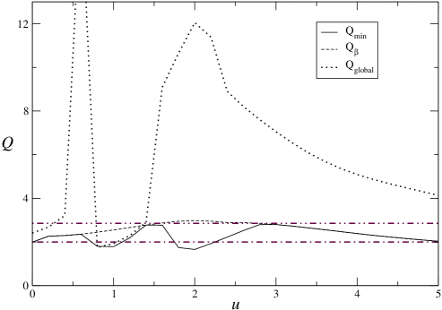
VI.2 Evolution for different gravitational initial data

Independently of the initial data $J$, the star settles into “quasi-equilibrium” after a couple of hydrodynamical times given by $2R_{*}$, i.e. all variables relax to roughly constant values with respect to a co-rotating observer. Of the small remaining variation, a major portion subsequently dies off after a couple of crossing times $2a$, the time needed for the star to communicate with the inner boundary and back. This latter behavior is observed whether or not the internal hydrodynamics of the star is evolved. After this relaxation period, the time dependence of the gravitational field is mainly determined by the motion of the star.

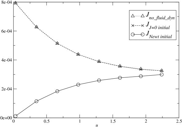
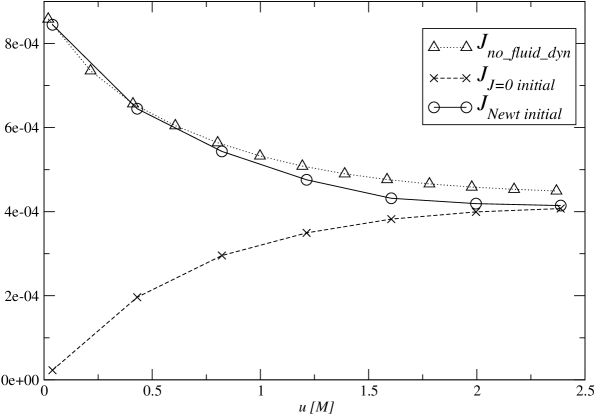
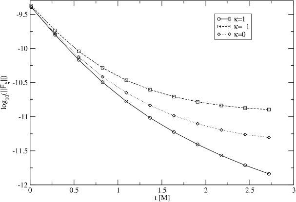
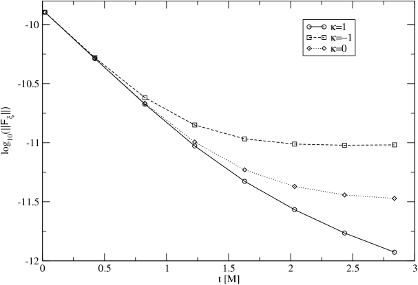
As an illustration of this behavior we evolve a star in a space-time both with and without a black hole. The star is placed at $a=9$ with mass $m=10^{-4}$ and radius $R_{*}=3$ and the gravitational initial data is given either by $J=0$ (shear-free data) or by the quasi-Newtonian value. For purposes of comparison, runs are made both with the hydrodynamic variables evolved and frozen. Figures 2 and 3 illustrate the behavior of $J$ for these cases. After a relatively brief transient behavior, the norm of $J$ approaches a value quite independent of the initial data (with similar behavior observed in all other gravitational field variables). This indicates that most of the spurious radiation present in the initial hypersurface is ‘flushed out’ in a short time. In order to elucidate whether the system settles into a quasi-stationary state, as might be expected, we analyze next whether there is an approximate helical Killing vector in the space-time.

Figure 2: Behavior of $||J||$ for the case with no black hole. Three scenarios are plotted: Full evolution (hydrodynamics + gravity) using initial data $J=0$ (dashed line with “x” symbols); full evolution using quasi-Newtonian initial data (solid line with circular symbols); and gravitational evolution with frozen internal hydrodynamics using quasi-Newtonian data (dotted lines with triangular symbols). After some transient behavior, lasting until about $u\sim 2$, all curves roughly approach the same value.

Figure 3: Behavior of $||J||$ for the case of an $M=1$ black hole. Again three scenarios are plotted: Full evolution using initial data $J=0$ (dashed line with “x” symbols); full evolution using quasi-Newtonian initial data (solid line with circular symbols); and gravitational evolution with frozen hydrodynamics using quasi-Newtonian data (dotted lines with triangular symbols). After some transient behavior lasting until $u\sim 2$, all curves roughly approach the same value.

Agreement of the “relaxed state”

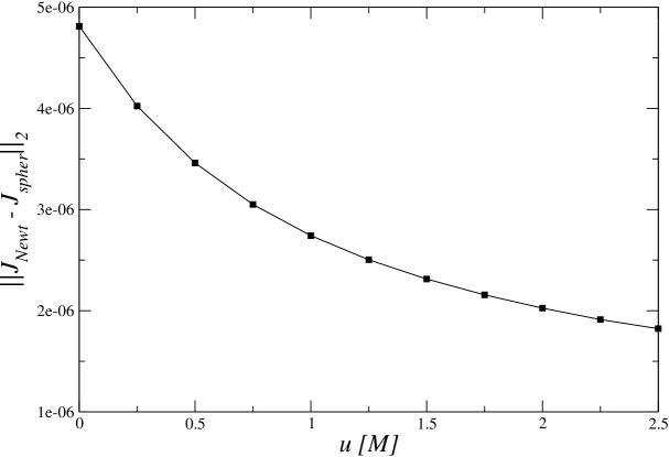
As indicated above, the system appears to relax to a state independent of the details of the initial data. In order to quantify this, we calculate the $L_{2}$ norm of the difference between the two numerical solutions obtained with Newtonian and with shear-free initial data. Figures 4 and 5 illustrate the behavior of the difference vs. time, showing how as time progresses the agreement between the numerical solutions becomes more pronounced.

Figure 4: $L_{2}$ norm of the difference between the computed values of $J$ for the quasi-Newtonian and spherically symmetric initial data.

It is also illustrative to observe the point-wise difference between the two numerical solutions. In particular, inspection of $|J_{Newt}-J_{spher}|$ at ${\cal I}^{+}$ reveals not only that the solutions tend to agree as time progresses, but also that this agreement is more marked along null rays passing through the star and neighboring rays.

Figure 5: Absolute value of the difference between the computed values of $J$ at ${\cal I}^{+}$ evolved from quasi-Newtonian and from shear-free initial data. The panels (A,B,C,D) correspond to the time sequence $u=0$, $u=0.75M$, $u=1.5M$, and $u=2.5M$. Panel A has been truncated for comparison purposes, as its height is $\approx 9\times 10^{-5}$.

VI.3 Quasi-equilibrium behavior

In order to measure the approach to quasi-equilibrium we monitor the rate of change of the angular part of the metric along the streamlines of the vector field $\xi=T+\kappa\Omega\Phi$. As explained in Sec. III.3.1, for $\kappa=1$, $\xi$ equals the helical Killing vector of the background black hole with $\Omega$ set to the initial orbital angular velocity of the star. For comparison purposes we also consider $\kappa=0$, for which $\xi$ equals the static Killing vector $T$ of the background black hole, and $\kappa=-1$, for which $\xi$ equals the helical Killing vector counter-rotating with respect to the orbital motion of the star. We measure the change of the gravitational field with respect to the flow of these vector fields by the norm $F_{\kappa}\equiv||{\cal L}_{\xi}h_{AB}||^{2}$. For orbital motion in quasi-equilibrium around the black hole, we should then find $F_{\kappa=1}\approx 0$. In order to verify that this is the case, we monitor the values of $F_{\kappa}$ for $\kappa=1,0,-1$. Again, the star is initialized at $a=9$ with mass $m=10^{-5}$ and radius $R_{*}=3$.

The first test, carried out with quasi-Newtonian initial data and shown in Figure 6, compares the behavior of $F_{\kappa}$ for the three different values of $\kappa$ indicated above. At first, the curves differ very little, but at later times there is a marked difference ($>1.5$ orders of magnitude), indicating that the system approaches an approximate helical symmetry. For the $\kappa=1$ helical case, $F_{1}$ decays more than two orders of magnitude from its initial value.

Figure 6: Comparison of $F_{\kappa}$ using quasi-Newtonian initial data.

Next we repeat the test with $J=0$ shear-free initial data, with the results shown in Fig. 7. The initial values of $F_{\kappa}$ are not the same as those in the first test, but a similar time behavior is observed. Again the helical choice $F_{1}$ decays more than two orders of magnitude from its initial value, and more than an order of magnitude more than either $F_{0}$ or $F_{-1}$.

Figure 7: Comparison of $F_{\kappa}$ using shear-free initial data.

VI.4 Co-rotating coordinates

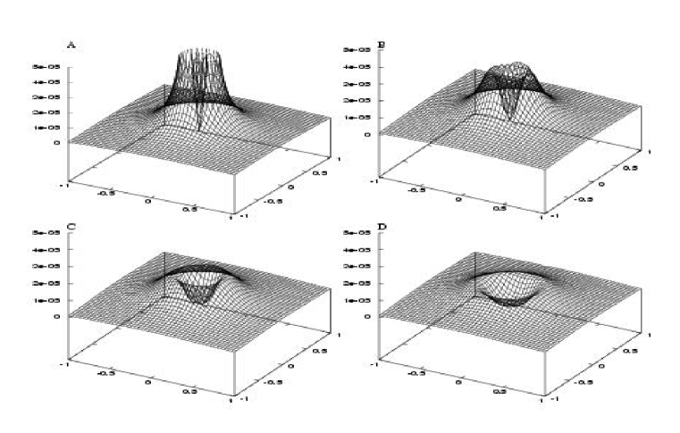
Co-rotating coordinates can improve the tracking and hydrodynamic treatment of the orbiting star by reducing or eliminating the variation of field values due to purely coordinate effects. They are introduced here by specifying the value of $U$ at the inner boundary, as described in section III.3.1. By defining $U$ via Eq. (36), we have checked that this indeed keeps the angular coordinate of the star fixed. The tests were carried out in the star mass range $m\in[10^{-7},10^{-2}]$, with $M=1$, $R_{*}=3M$ and $a=9M$. Figure 8 illustrates the results for $m=10^{-5}$. As can be seen clearly from the density contours displayed, the co-rotating coordinates maintain the central density of the star at the same initial coordinate location after evolution through $u=2.8$. Note that, although the initial polytrope is spherically symmetric about the center of the star, the kinetic energy contributed by the initially uniform orbital angular velocity skews the density distribution. These results verify that the initialization can be performed equally well in co-rotating coordinates.

Figure 8: For the case $m=10^{-5}$, $R_{*}=3M$, $a=9M$ we show density profiles in the plane with stereographic coordinate $p=0$. The motion takes place in the $(r,q)$ plane. In all figures, the vertical axis is $x$ (the compactified radial coordinate)and the horizontal axis is $q$. The top panels correspond to the fixed coordinates (A) and co-rotating coordinates (B) at the initial time $u=0$. Figures (C) and (D) show the corresponding density profiles at $u=2.8$. The co-rotating coordinates, panel (D), perform well in keeping the coordinate location of the star fixed. For comparison, panel (C) shows the actual displacement of the star.

VI.5 Monitoring the expansion of the null coordinates

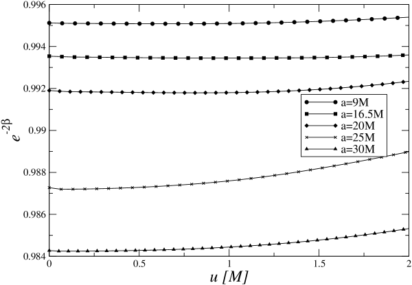
When the star is initialized sufficiently far from the central black hole, its bending effect on neighboring light rays can cause a coordinate singularity, by reducing the expansion of the outgoing null hypersurfaces to zero. As discussed in Sec. IV, the bending effect on outgoing null rays is first evident at future null infinity, where it is manifested in our formalism by $\beta\rightarrow\infty$. However, $\beta\rightarrow\infty$ also when the generators of the outgoing null hypersurfaces approach a black hole horizon, in which case $\beta\rightarrow\infty$ on a complete spherical set of rays. As a result, it is difficult to distinguish at a given retarded time between whether it is a horizon or a coordinate singularity that is responsible for the lack of expansion. In the present context, what matters is whether such coordinate singularities can arise on a relatively short dynamical time scale which would have bearing on our main conclusion that the system relaxes to a quasi-stationary orbit. To assess this possibility, we carry out evolutions with a star of mass $m=10^{-3}M$ and radius $R_{*}=3M$ initially placed in orbit at different distances $a$ from the central black hole. We then monitor the expansion $e^{-2\beta}$ for roughly the “relaxation” time. Figure 9 graphs the $u$-dependence of the minimum value of $e^{-2\beta}$ over the sphere at null infinity for the initial orbital radii $a=9M,16.5M,20M,25M,30M$. As expected, the expansion becomes smaller as the separation between the star and the black hole increases. More important to the initialization problem, for a given separation the minimum expansion does not appear to change considerably from its initial value during the relaxation time. An estimate obtained with the lens equation combined with the initial value of $\beta$ at infinity seems to provide a good indicator of whether coordinate singularities will develop.

Figure 9: Time behavior of the minimum expansion $e^{2\beta}$ at future null infinity vs. initial location of the star. As the star is placed farther from the black hole its focusing effect on the central null rays increases. However, the expansion stays close to its initial value for a given separation $a$.

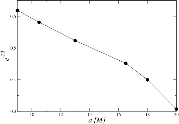
We now examine the possibility of dealing with a more massive star $m=10^{-1}M$, keeping $R_{*}=3M$. The lens estimate predicts zero expansion at a separation given by $a\geq 22.5M$. To study this problem, we set up data at different separations and, in view of the behavior just seen in the case with $m=10^{-3}M$, we evolve for a short time ($u=M/10$). Figure 10 graphs the computed value of $e^{-2\beta}$ vs. $a$, for a range of separations. As the star is placed farther from the black hole, the expansion gets considerably smaller. Furthermore, the values obtained for $a>16M$ only represent an upper bound since even with the largest practical grid $nr\times nq\times np=132\times 82^{2}$ the star is considerably unresolved. As a result, the neighboring null rays pass by the star at a significant “grid distance” and do not accurately represent the expansion that would be calculated in the continuum problem. Nevertheless, the results in the figure suggest that it would be possible to simulate a star in orbit around a black hole with $a<16M$ on a uniform grid without developing coordinate problems.

Figure 10: Behavior of the minimum of the expansion $e^{-2\beta}$ at future null infinity vs. location of the star. As the star’s initial location is placed farther from the black hole its focusing effect on the central null rays becomes considerably.

VI.6 Code performance

We illustrate the speed of the code for the case of the finest grid used in the convergence test, i.e. $81^{2}\times 123$. Setting the time-step to $\Delta u=0.014M$, a run until $u=1.5M$ takes 9 hours on a 2.4GHz Pentium 4 processor, and requires 1.4Gb of memory. From this we conclude that a single orbit would take roughly 1 1/2 months.

VII Conclusion

Within the characteristic framework, we have developed and implemented a numerical relativity code, as well as procedures for finding the required initial data, for evolving a star in close orbit around a Schwarzschild black hole. We have shown that after a short evolution time the system relaxes to a quasi-equilibrium state which is mainly independent of the initial gravitational data. Variations of the initial matter data, such as the shape or size of the star, have not been investigated. For small variations about stellar equilibrium one would expect similar results since the accompanying variations in the star’s gravitational field should relax to the same quasi-equilibrium state. We have also developed and demonstrated tools that permit the use of co-rotating coordinates and that monitor possible problems with the null coordinate system.

Successful simulation of a neutron star in close orbit around a black hole requires a gravity code, a hydrodynamic code and physically appropriate initial data. It has already been demonstrated that the characteristic gravity code is accurate and stable hpn ; roberto . In this paper we have implemented and tested a conservative formulation of the hydrodynamics and used it to shed light on the problem of prescribing physically meaningful initial data. There are several issues that remain to be addressed before physically interesting long term evolutions can be carried out. The results obtained in this paper would appear to justify the effort required to make these improvements.

Specifically, in order for the code to yield astrophysically useful results, three further conditions must be fulfilled. First, more realistic inner boundary data must be provided. This must correspond to a spinning black hole and must include the gravitational distortion induced by the companion star. Second, the turn-around of results must be considerably improved. This will require revising the numerical algorithms and parallelization of the code to take advantage of large platforms. Finally, since accurate simulations require that the numerical error be well below the expected radiation output ($<5$%), the use of adaptive mesh refinement seems crucial. Preliminary work in this direction has recently been presented nullamr . All of these items are major tasks and are deferred to future work.

Appendix A Computation of the quasi-Newtonian initial data

The Newtonian potential outside the polytrope is simply

$$\Phi=-\frac{m}{R}\;\;\;(R>R_{*}).$$ (49)

Inside the polytrope, the derivation is rather more complicated. We find

$$\Phi=-\frac{m}{R_{*}}-\frac{m\sin{\frac{R\pi}{R_{*}}}}{R\pi}\;\;\;(R<R_{*}).$$ (50)

and from it obtained $\eth^{2}\Phi$. First, we make the following definitions

$$z = q+ip$$

$$t_{1} = (r-a)^{2}+z\bar{z}(r+a)^{2}$$

$$P_{p} = 1+z\bar{z}$$

$$t_{2} = \frac{\pi}{R_{*}}\sqrt{\frac{t_{1}}{P_{p}}}$$

$$t_{3} = \frac{a^{2}r^{2}z^{2}m\sqrt{P_{p}}}{t_{1}^{5/2}}.$$ (51)

Then we may write

$$\eth^{2}\Phi = -12t_{3}\;\;\;(R>R_{*})$$

$$\eth^{2}\Phi = -4\frac{t_{3}}{R_{*}^{2}\pi}\times$$ (52)

$$\left((-\pi^{2}r^{2}+2r\pi^{2}a\frac{1-z\bar{z}}{P_{p}}+3R_{*}^{2}-\pi^{2}a^{2})\sin{t_{2}}-3R_{*}\pi\sqrt{\frac{t_{1}}{P_{p}}}\cos{t_{2}}\right)$$

$$(R<R_{*}).$$

Finally, $J$ is obtained by numerically integrating $(r^{2}J_{,r})_{,r}=-2\eth^{2}\Phi$ in second order form starting from the inner boundary $r=2M$.

References

- (1) M. J. Rees, in Proceedings of the 18th Texas Symposium, edited by A. Olinto, J. Frieman and D. Schramm (World Scientific, Singapore, 1998).
- (2) C. Cutler and K.S. Thorne, in Proceedings of the 16th International Conference on General Relativity & Gravitation, edited by N.T. Bishop and S.D. Maharaj (World Scientific, Singapore, 2002).
- (3) M. Vallisneri, Phys. Rev. Lett. 84, 3519 (2000).
- (4) M. B. Davies, A. J. Levan and A. R. King, “The ultimate outcome of black hole - neutron star mergers”, Mon. Not. R. Astron. Soc, to appear, astro-ph/0409681.
- (5) T. Baumgarte, private communication.
- (6) M. Shibata, private communication.
- (7) M. Miller, private communication.
- (8) I. Hawke, private communication.
- (9) F. Siebel, J. A. Font, E. Muller and P. Papadopoulos, Phys. Rev. D 67, 124018 (2003).
- (10) F. Siebel, J. A. Font and P. Papadopoulos, Phys. Rev. D 65, 024021 (2002).
- (11) N.T. Bishop, R. Gómez, L. Lehner, M. Maharaj, and J. Winicour, Phys. Rev. D 56, 6298 (1997).
- (12) N.T. Bishop, R. Gómez, L. Lehner, M. Maharaj, and J. Winicour, Phys. Rev. D 60, 024005 (1999).
- (13) C. Klein, Binary black hole spacetimes with a helical Killing vector, Phys. Rev. D, to appear, gr-qc/0410095.
- (14) M. Shibata, K. Uryu and J. L. Friedman, Phys. Rev. D 70, 044044 (2004).
- (15) H. J. Yo, J. N. Cook, S. L. Shapiro, and T. W. Baumgarte, Phys. Rev. D 70, 084033 (2004).
- (16) Z. Andrade et. al., Phys. Rev. D 70, 064001 (2004).
- (17) E. Gourgoulhon, P. Grandclément and S. Bonazzola, Phys. Rev. D 65, 044020 (2002).
- (18) R. J. Leveque, Numerical Methods for Conservation Laws (Birkhauser-Verlag, Basel, 1990).
- (19) P. Papadopoulos and J. A. Font, Phys. Rev. D 61, 024015 (2000).
- (20) S. Davis, Siam J. Sci. Stat. Comput., 8, 1, (1987).
- (21) J. Winicour, J. Math. Phys. 24, 1193 (1983).
- (22) J. Winicour, J. Math. Phys. 24, 2506 (1983).
- (23) R.A. Isaacson, J.S. Welling, and J. Winicour, J. Math. Phys. 26, 2859 (1985).
- (24) J. Winicour, J. Math. Phys. 28, 668 (1987).
- (25) N.T. Bishop, R. Gómez, L. Lehner, and J. Winicour, Phys. Rev. D 54, 6153 (1996).
- (26) R.A. Isaacson, J.S. Welling, and J. Winicour, J. Math. Phys. 24, 1824 (1983).
- (27) N.T. Bishop, Class. Quantum Grav. 10, 333 (1993).
- (28) N.T. Bishop C.J.S. Clarke, and R.A. d’Inverno, Class. Quantum Grav. 7, L23 (1993).
- (29) H. Bondi, M.J.G. van der Burg and A.W.K. Metzner, Proc. R. Soc. A 269 21, (1962).
- (30) R.K. Sachs, Proc. R. Soc. London A 270, 103 (1962).
- (31) L.A. Tamburino and J. Winicour, Phys. Rev. 150, 1039, (1966).
- (32) R. Gómez, Phys. Rev. D 64, 024007 (2001).
- (33) N.T. Bishop, R. Gómez, S. Husa, L. Lehner, and J. Winicour, Phys. Rev. D 68, 084015 (2003)
- (34) Y. Zlochower, R. Gómez, S. Husa, L. Lehner and J. Winicour, Phys. Rev. D 68, 084014 (2003).
- (35) R. Gómez, L. Lehner, P. Papadopoulos and J. Winicour, Class. Quantum Grav. 14, 977, (1997).
- (36) S. Chandrasekhar, An introduction to the study of stellar structure (Dover, New York, 1967).
- (37) K. Uryu and Y. Eriguchi, Mon. Not. R. Astron. Soc. 303, 329 (1999).
- (38) J.C. Lombardi, F.A. Rasio, S.L. Shapiro, Phys. Rev. D 56, 3416 (1997).
- (39) R. Gómez, S. Husa and J. Winicour, Phys. Rev. D 64, 0240010 (2001).
- (40) R. Gómez, L. Lehner, R. L. Marsa and J. Winicour, Phys. Rev. D 57, 4778 (1998).
- (41) R. Gómez, S. Husa, L. Lehner and J. Winicour, Phys. Rev. D 66, 064019 (2002).
- (42) F. Pretorius and L. Lehner, J. Comput. Phys. 198, 10 (2004).
- (43) S. Dain, “A new geometric invariant on initial data for Einstein equations”, preprint, arXiv:gr-qc/0406099.