New class of post-Newtonian approximants to the waveform templates of inspiralling compact binaries: Test-mass in the Schwarzschild spacetime

Abstract

The standard adiabatic approximation to phasing of gravitational waves from inspiralling compact binaries uses the post-Newtonian expansions of the binding energy and gravitational wave flux both truncated at the same relative post-Newtonian order. Motivated by the eventual need to go beyond the adiabatic approximation we must view the problem as the dynamics of the binary under conservative post-Newtonian forces and gravitational radiation damping. From the viewpoint of the dynamics of the binary, the standard approximation at leading order is equivalent to retaining the 0PN and 2.5PN terms in the acceleration and neglecting the intervening 1PN and 2PN terms. A complete mathematically consistent treatment of the acceleration at leading order should include all PN terms up to 2.5PN without any gaps. These define the standard and complete non-adiabatic approximants respectively. We propose a new and simple complete adiabatic approximant constructed from the energy and flux functions. At the leading order it uses the 2PN energy function rather than the 0PN one in the standard approximation so that in spirit it corresponds to the dynamics where there are no missing post-Newtonian terms in the acceleration. We compare the overlaps of the standard and complete adiabatic approximant templates with the exact waveform (in the adiabatic approximation) for a test-particle orbiting a Schwarzschild black hole. Overlaps are computed using both the white-noise spectrum and the initial LIGO noise spectrum. The complete adiabatic approximants lead to a remarkable improvement in the effectualness (i.e. larger overlaps with the exact signal) at lower PN ($<$ 3PN) orders. However, standard adiabatic approximants of order $\geq$ 3PN are nearly as good as the complete adiabatic approximants for the construction of effectual templates. In general, faithfulness (i.e. smaller biases in the estimation of parameters) of complete approximants is also better than that of standard approximants. Standard and complete approximants beyond the adiabatic approximation are next studied using the Lagrangian models of Buonanno, Chen and Vallisneri in the test mass limit. A limited extension of the results to the case of comparable mass binaries is provided. In this case, standard adiabatic approximants achieve an effectualness of 0.965 at order 3PN. If the comparable mass case is qualitatively similar to the test mass case then neither the improvement of the accuracy of energy function from 3PN to 4PN nor the improvement of the accuracy of flux function from 3.5PN to 4PN will result in a significant improvement in effectualness in the comparable mass case for terrestrial laser interferometric gravitational wave detectors.

I Introduction

The late-time dynamics of astronomical binaries consisting of neutron stars and/or black holes is dominated by relativistic motion and non-linear general relativistic effects. The component bodies would be accelerated to velocities close to half the speed of light before they plunge towards each other, resulting in a violent event during which the source would be most luminous in the gravitational window. Such events are prime targets of interferometric gravitational wave (GW) detectors like LIGO/VIRGO/GEO/TAMA that are currently taking data at unprecedented sensitivity levels and bandwidths ligo ; virgo ; geo ; tama .

Binary coalescences are the end state of a long period of adiabatic dynamics in which the orbital frequency of the system changes as a result of gravitational radiation backreaction but the change in frequency per orbit is negligible compared to the orbital frequency itself. Indeed, the adiabatic inspiral phase is well-modelled by the post-Newtonian (PN) approximation to Einstein’s equations but this approximation becomes less accurate close to the merger phase. Additionally, there are different ways of casting the gravitational wave phasing formula – the formula that gives the phase of the emitted gravitational wave as a function of time and the parameters of the system. These different approaches make use of the post-Newtonian expansions of the binding energy and gravitational wave luminosity of the system.

I.1 Standard approach to phasing formula

The standard approach in deriving the phasing formula uses the specific gravitational binding energy $E(v)$ (i.e. the binding energy per unit mass) of the system and its luminosity ${\cal F}(v),$ both to the same relative accuracy CF . Including the radiation reaction at dominant order, however, is not a first order correction to the dynamics of the system, rather it is a correction that arises at ${\cal O}[(v/c)^{5}],$ where $v$ is the post-Newtonian expansion parameter describing the velocity in the system and $c$ is the speed of light . Thus, the phasing of the waves when translated to the relative motion of the bodies implies that the dynamics is described by the dominant Newtonian force and a correction at an order $(v/c)^{5},$ but neglecting conservative force terms that occur at orders $(v/c)^{2}$ and $(v/c)^{4}.$ Such considerations have led to an approximation scheme in which one constructs the phasing of gravitational waves using the following ordinary, coupled differential equations:

$$\frac{d\varphi}{dt}=\frac{2v^{3}}{m},\ \ \ \ \frac{dv}{dt}=-\frac{{\cal F}(v)}{mE^{\prime}(v)},$$ (1)

where $E^{\prime}(v)=dE(v)/dv$ and $m=m_{1}+m_{2}$ is the total mass of the binary. The phasing obtained by numerically solving the above set of differential equations is called the TaylorT1 approximant dis03 . If the detector’s motion can be neglected during the period when the wave passes through its bandwidth then the response of the interferometer to arbitrarily polarized waves from an inspiralling binary is given by

$$h(t)=\frac{4A\eta m}{D}v^{2}(t)\cos[\varphi(t)+\varphi_{C}],$$ (2)

where $\varphi(t)$ is defined so that it is zero when the binary coalesces at time $t=t_{C},$ $\varphi_{C}$ is the phase of the signal at $t_{C},$ $\eta=m_{1}m_{2}/m^{2}$ is the symmetric mass ratio, $D$ is the distance to the source and $A$ is a numerical constant whose value depends on the relative orientations of the interferometer and the binary orbit. It suffices to say for the present purpose that for an optimally oriented source $A=1.$

One can compute the Fourier transform $H(f)$ of the waveform given in Eq. (2) using the stationary phase approximation:

$$H(f)=\frac{4Am^{2}}{D}\sqrt{\frac{5\pi\eta}{384}}v_{f}^{-7/2}e^{i\left[2\pi ft_{C}-\varphi_{C}+\psi(f)-\pi/4\right]},$$ (3)

where the phase of the Fourier transform obeys a set of differential equations given by

$$\frac{d\psi}{df}=2\pi t,\ \ \ \ \frac{dt}{df}=-\frac{\pi m^{2}}{3v_{f}^{2}}\frac{E^{\prime}(v_{f})}{{\cal F}(v_{f})}.$$ (4)

In the above expressions, including the post-Newtonian expansions of the energy and flux functions, the parameter $v_{f}=(\pi mf)^{1/3}$. The waveform Eq.(3) computed by numerically solving the differential equations Eq.(4) is called TaylorF1 dis03 approximant.

Before we proceed further, let us recall the notation used in post-Newtonian theory to identify different orders in the expansion. In the conservative dynamics of the binary, wherein there is no dissipation, the energy is expressed as a post-Newtonian expansion in $\epsilon=(v/c)^{2},$ with the dominant order termed Newtonian or 0PN and a correction at order $\epsilon^{n}=(v/c)^{2n},$ $n=1,2,\ldots,$ called $n$PN, with the dynamics involving only even powers of $\sqrt{\epsilon}=(v/c).$ When dissipation is added to the dynamics, then the equation of motion will have terms of both odd and even powers of $v/c$. Thus, a correction of order $(v/c)^{m}$ is termed as $(m/2)$PN.

In the adiabatic approximation of a test-particle orbiting a Schwarzschild black hole, the energy function $E(v)$ is exactly calculable analytically, while the flux function ${\cal F}(v)$ is exactly calculable numerically P93 ; P95 ; TagNak ; shibata93 . In addition, ${\cal F}(v)$ has been calculated analytically to 5.5PN order TTS97 by black hole perturbation theory ST-LivRev . In contrast, in the case of a general binary including bodies of comparable masses, the energy function $E(v)$ has been calculated recently to 3PN accuracy by a variety of methods DJS ; BF ; DJS02 ; BDE03 ; IF ; itoh2 . The flux function ${\cal F}(v),$ on the other hand, has been calculated to 3.5PN accuracy BDIWW ; BDI ; WW ; BIWW ; B96 ; BIJ02 ; BFIJ02 ; ABIQ04 ; BDEI ; BI04 ; BDI04 up to now only by the multipolar-post-Minkowskian method and matching to a post-Newtonian source Luc-LivRev .

I.2 Complete phasing of the adiabatic inspiral: An alternative

The gravitational wave flux arising from the lowest order quadrupole formula, that is the 0PN order flux, leads to an acceleration of order 2.5PN in the equations-of-motion. This far-zone computation of the flux requires a control of the dynamics, or acceleration, to only Newtonian accuracy. The lowest order GW phasing in the adiabatic approximation uses only the leading terms in the energy (Newtonian) and flux (quadrupolar) functions. For higher order phasing, the energy and flux functions are retained to the same relative PN orders. For example, at 3PN phasing, both the energy and flux functions are given to the same relative 3PN order beyond the leading Newtonian order. We refer to this usual physical treatment of the phasing of GWs computed in the adiabatic approximation, and used in the current LIGO/VIRGO/GEO/TAMA searches for the radiation from inspiralling compact binaries, as the standard adiabatic approximation. We will denote the $n$PN standard adiabatic approximant as $T(E_{[n]},{\cal F}_{n})$, where $[p]$ denotes the integer part of $p$.

As a prelude to go beyond the standard adiabatic approximation, let us consider the phasing of the waves in terms of the equations of motion of the system. To this end, it is natural to order the PN approximation in terms of its dynamics or acceleration. From the viewpoint of the dynamics, the leading order standard adiabatic approximation is equivalent to using the 0PN (corresponding to 0PN conserved energy) and 2.5PN (corresponding to the Newtonian or 0PN flux) terms in the acceleration ignoring the intervening 1PN and 2PN terms. A complete, mathematically consistent treatment of the acceleration, however, should include all PN terms in the acceleration up to 2.5PN, without any gaps. We refer to the dynamics of the binary, and the resulting waveform, arising from the latter as the 0PN complete non-adiabatic approximation. In contrast, the waveform arising from the former choice, with gaps in the acceleration at 1PN and 2PN, is referred to as the 0PN standard non-adiabatic approximation. Extension to higher-order phasing is obvious. At 1PN the standard non-adiabatic approximation would involve acceleration terms at orders 0PN, 1PN, 2.5PN and 3.5PN, whereas the complete non-adiabatic approximation would additionally involve the 2PN and 3PN acceleration terms.

Finally, we propose a simple extension of the above construction to generate a new class of approximants in the adiabatic regime. To understand the construction let us examine the lowest order case. Given the 0PN flux (leading to an acceleration at 2.5PN), one can choose the energy function at 2PN (equivalent to 2PN conservative dynamics) instead of the standard choice 0PN (equivalent to 0PN or Newtonian conservative dynamics). This is the adiabatic analogue of the complete non-adiabatic approximant. Extension to higher PN orders follows naturally. For instance, corresponding to the flux function at 1PN (1.5PN), the dissipative force is at order 3.5PN (4PN), and, therefore, the conservative dynamics, and the associated energy function, should be specified up to order 3PN (4PN). In general, given the flux at $n$PN-order, a corresponding complete adiabatic approximant is constructed by choosing the energy function at order $[n+2.5]$PN, where as mentioned before, $[p]$ denotes the integer part of $p$. We refer to the dynamics of the binary and the resulting waveform arising from such considerations, as the complete adiabatic approximation. We will denote the $n$PN complete adiabatic approximant as $T(E_{[n+2.5]},{\cal F}_{n})$.

Before moving ahead the following point is worth emphasizing: The standard adiabatic phasing is, by construction, consistent in the relative PN order of its constituent energy and flux functions, and thus unique in its ordering of the PN terms. Consequently, one can construct different inequivalent, but consistent, approximations as discussed in Ref. dis03 by choosing to retain the involved functions or re-expand them. The complete adiabatic phasing, on the other hand, is constructed so that it is consistent in spirit with the underlying dynamics, or acceleration, rather than with the relative PN orders of the energy and flux functions. Consequently, it has a unique meaning only when the associated energy and flux functions are used without any further re-expansions when working out the phasing formula. As a result, though the complete non-adiabatic approximant is more consistent than the standard non-adiabatic approximant in treating the PN accelerations, in the adiabatic case there is no rigorous sense in which one can claim that either of the approximants is more consistent than the other. The important point, as we shall see is that, not only are the two approximants not the same but the new complete adiabatic approximants are closer to the exact solution than the standard adiabatic approximants.

In our view, these new approximants should be of some interest. They are simple generalizations of the standard adiabatic approximants coding information of the PN dynamics beyond the standard approximation without the need for numerical integration of the equations of motion. They should be appropriate approximants to focus on when one goes beyond the adiabatic picture and investigates the differences stemming from the use of more complete equations of motion (see Section III).

In the case of comparable mass binaries, the energy function is currently known up to 3PN order and hence it would be possible to compute the complete adiabatic phasing of the waves to only 1PN order. One is thus obliged in practice to follow the standard adiabatic approximation to obtain the phasing up to 3.5PN order. Consequently, it is a relevant question to ask how ‘close’ are the complete and standard adiabatic approximants. The standard adiabatic approximation would be justified if we can verify that it produces in most cases a good lower bound to the mathematically consistent, but calculationally more demanding, complete adiabatic approximation. In this paper we compare the standard and complete models by explicitly studying their overlaps with the exact waveform which can be computed in the adiabatic approximation of a test mass motion in a Schwarzschild spacetime. The availability, in this case, of the exact (numerical) and approximate (analytical) waveforms to as high a PN order as $(v/c)^{11}$, allows one to investigate the issue exhaustively, and provides the main motivation for the present analysis. Assuming that the comparable mass case is qualitatively similar and a simple $\eta$-distortion of the test mass case would then provide a plausible justification for the standard adiabatic treatment of the GW phasing employed in the literature.

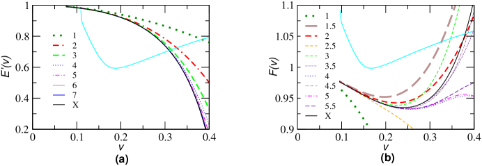
Figure 1: Various T-approximants of Newton-normalized ($v$-derivative of) energy function $E^{\prime}_{\rm T}(v)/E^{\prime}_{\rm N}(v)$ (left), and flux function ${\cal F}_{\rm T}(v)/{\cal F}_{\rm N}(v)$ (right) in the test mass limit along with the exact functions (denoted by $X$). Also plotted is the amplitude spectral density (per $\sqrt{\rm Hz}$) of initial LIGO noise in arbitrary units.

I.3 Non-adiabatic inspiral

The phasing formulas derived under the various adiabatic approximation schemes assume that the orbital frequency changes slowly over each orbital period. In other words, the change in frequency $\Delta\nu$ over one orbital period $P$ is assumed to be much smaller than the orbital frequency $\nu\equiv P^{-1}.$ Denoting by $\dot{\nu}$ the time-derivative of the frequency, the adiabatic approximation is equivalent to the assumption that $\Delta\nu=\dot{\nu}P\ll\nu$ or $\dot{\nu}/\nu^{2}\ll 1.$ This assumption becomes somewhat weaker, and it is unjustified to use the approximation $\dot{E}=-{\cal F},$ when the two bodies are quite close to each other. Buonanno and Damour bd99 ; bd00 introduced a non-adiabatic approach to the two-body problem called the effective one-body (EOB) approximation. In this approximation one solves for the relative motion of the two bodies using an effective Hamiltonian with a dissipative force put-in by hand. EOB allows to extend the dynamics beyond the adiabatic regime, and the last stable orbit, into the plunge phase of the coalescence of the two bodies bd00 ; DGG ; GGB1 ; GGB2 .

Recently, Buonanno, Chen and Vallisneri BCV02 have studied a variant of the non-adiabatic model but using the effective Lagrangian constructed in the post-Newtonian approximation. We shall use both the standard and complete non-adiabatic Lagrangian models in this study and see how they converge to the exact waveform defined using the adiabatic approximation.

I.4 What this study is about

In our study we will use the effectualness and faithfulness (see below) to quantify how good the various approximation schemes are. There are at least three different contexts in which one can examine the performance of an approximate template family relative to an exact one. Firstly, one can think of a mathematical family of approximants and examine its convergence towards some exact limit. Secondly, one can ask whether this mathematical family of approximants correctly represents the GWs from some physical system. Thirdly, how does this family of approximate templates converge to the exact solution in the sensitive bandwidth of a particular GW detector. In the context of GW data analysis, the third context will be relevant and studied in this paper. Although there is no direct application to GW data analysis, equally interesting is the mathematical question concerning the behavior of different approximations, and the waveforms they predict, in the strongly non-linear regime of the dynamics of the binary, which is also studied in this paper. The latter obviously does not require the details of the detector-sensitivity and it is enough to study the problem assuming a flat power spectral density (i.e. a white-noise background) for the detector noise.

To summarize, our approach towards the problem will be two-pronged. First, we will study the problem as a general mathematical question concerning the nature of templates defined using PN approximation methods. We shall deal with four families of PN templates – the standard adiabatic, complete adiabatic, standard non-adiabatic and complete non-adiabatic (in particular, Lagrangian-based) approximants – and examine their closeness, defined by using effectualness and faithfulness, to the exact waveform defined in the adiabatic approximation. Since this issue is a general question independent of the characteristics of a particular GW detector, we first study the problem assuming the white-noise case. Having these results, we then proceed to see how and which of these results are applicable to a specific detector, namely the initial LIGO . During the course of this study, we also attempt to assess the relative importance of improving the accuracy of the energy and flux functions by studying the overlaps of the PN templates constructed from different orders of energy and flux functions with the exact waveform. It should be kept in mind that this work is solely restricted to the inspiral part of the signal and neglects the plunge and quasi-normal mode ringing phases of the binary FH98 ; bd00 ; dis03 ; BCV02 ; DIJS ; QNM .

I.5 Effectualness and Faithfulness

In order to measure the accuracy of our approximate templates we shall compute their overlap with a fiducial exact signal. We shall consider two types of overlaps dis01 ; dis02 ; dis03 ; dis04 . The first one is the faithfulness which is the overlap of the approximate template with the exact signal computed by keeping the intrinsic parameters (e.g. the masses of the two bodies) of both the template and the signal to be the same but maximizing over the extrinsic (e.g. the time-of-arrival and the phase at that time) parameters. The second one is the effectualness which is the overlap of the approximate template with the exact signal computed by maximizing the overlap over both the intrinsic and extrinsic parameters. Faithfulness is a measure of how good is the template waveform in both detecting a signal and measuring its parameters. However, effectualness is aimed at finding whether or not an approximate template model is good enough in detecting a signal without reference to its use in estimating the parameters. As in previous studies, we take overlaps greater than 96.5% to be indicative of a good approximation.

I.6 Organization of the paper

In the next section we study the test-mass waveforms in the adiabatic approximation. We discuss the construction of the exact energy and flux functions as well as the respective T-approximants. The overlaps of various standard adiabatic and complete adiabatic approximants are also compared in this Section. Section III deals with the non-adiabatic approximation. Section IV explores the extension of the results in the comparable mass case. It presents the energy and flux functions which are the crucial inputs for the construction of the fiducial ‘exact’ waveform as well as the approximate waveforms followed by a discussion of the results. In the last section we summarize our main conclusions.

One of the main conclusions of this paper is that the effectualness of the test-mass approximants significantly improves in the complete adiabatic approximation at PN orders below 3PN. However, standard adiabatic approximants of order $\geq$ 3PN are nearly as good as the complete adiabatic approximants for the construction of effectual templates. In the comparable mass case the problem can be only studied at the lowest two PN orders. No strong conclusions can be drawn as in the test mass case. Still, the trends indicate that the standard adiabatic approximation provides a good lower bound to the complete adiabatic approximation for the construction of both effectual and faithful templates at PN orders $\geq$ 1.5PN. From the detailed study of test-mass templates we also conclude that, provided the comparable mass case is qualitatively similar to the test mass case, neither the improvement of the accuracy of energy function from 3PN to 4PN nor the improvement of the accuracy of flux function from 3.5PN to 4PN will result in a significant improvement in effectualness in the comparable mass case. As far as faithfulness is concerned, it is hard to reach any conclusion. To achieve the target sensitivity of 0.965 in effectualness corresponding to a 10% loss in the event-rate, standard adiabatic approximants of order 2PN and 3PN are required for the $(10M_{\odot},10M_{\odot})$ and $(1.4M_{\odot},1.4M_{\odot})$ binaries, respectively, when restricting to only the inspiral phase. (Be warned that this is not a good approximation in the BH-BH case since the approach to the plunge and merger lead to significant differences.)

II Test mass waveforms in the adiabatic approximation

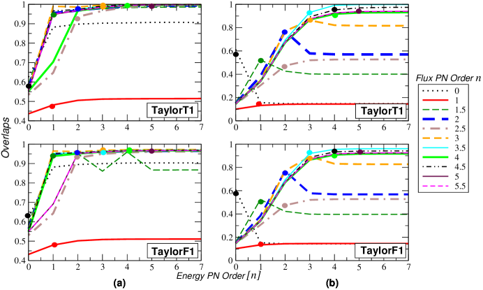
Figure 2: Effectualness (left panels) and faithfulness (right panels) of various test mass TaylorT1 and TaylorF1 templates in detecting a signal from a $(1M_{\odot},10M_{\odot})$ binary in white-noise. Different lines in the panels correspond to different orders of the flux function. Each line shows how the overlaps are evolving as a function of the accuracy of the energy function. Standard adiabatic approximants $T(E_{[n]},{\cal F}_{n})$ are marked with thick dots.

Our objective is to compare the effectualness (i.e larger overlaps with the exact signal) and faithfulness (i.e. smaller bias in the estimation of parameters) of the standard adiabatic $T(E_{[n]},{\cal F}_{n})$ and complete adiabatic $T(E_{[n+2.5]},{\cal F}_{n})$ approximants. As a by-product of this study, we would also like to have an understanding of the the relative importance of improving the accuracy of the energy function and flux function. Thus, what we will do is to take all possible combinations of T-approximants of energy and flux functions, construct PN templates and calculate the overlap of these templates with the exact waveform. In all cases, the exact waveform is constructed by numerically integrating the phasing formula in the time-domain [TaylorT1 approximant, cf. Eqs. (1) and (2)]. The waveforms (both the exact and approximate) are all terminated at $v_{\rm lso}=1/\sqrt{6},$ which corresponds to $F_{\rm lso}\simeq 43$ Hz for the $(1M_{\odot},100M_{\odot})$ binary, $F_{\rm lso}\simeq 86$ Hz for the $(1M_{\odot},50M_{\odot})$ binary and $F_{\rm lso}\simeq 399$ Hz for the $(1M_{\odot},10M_{\odot})$ binary . The lower frequency cut-off of the waveforms is chosen to be $F_{\rm low}=20$ Hz.

In this study, we restrict to approximants TaylorT1 and TaylorF1 since they do not involve any further re-expansion in the phasing formula and hence there is no ambiguity when we construct the phasing of the waves using approximants with unequal orders of the energy and flux functions.

II.1 The energy function

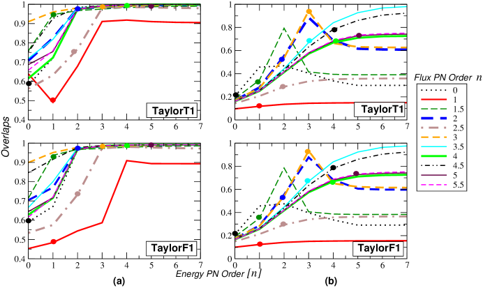
Figure 3: As in Fig. 2 except that the signal corresponds to a $(1M_{\odot},50M_{\odot})$ binary.

In the case of a test-particle $m_{2}$ moving in circular orbit in the background of a Schwarzschild black hole of mass $m_{1}$, where $m_{2}/m_{1}\rightarrow 0$, the energy function $E(x)$ in terms of the invariant argument $x\equiv v^{2}$ is given by

$$E_{\rm exact}(x)=\eta\,\frac{1-2x}{\sqrt{1-3x}}\,,$$ (5)

The associated $v$-derivative entering the phasing formula is

$$E_{\rm exact}^{\prime}(v)=2v\left.\frac{dE(x)}{dx}\right|_{x=v^{2}}=-\eta v\,\frac{(1-6\,v^{2})}{(1-3\,v^{2})^{3/2}}\,.$$ (6)

We use the above exact $E^{\prime}(v)$ to construct the exact waveform in the test-mass case. In order to construct various approximate PN templates, we Taylor-expand $E_{\rm exact}^{\prime}(v)$ and truncate it at the necessary orders.

$$E^{\prime}_{7PN}(v) = -\eta v\left[1-\frac{3\,v^{2}}{2}-\frac{81\,v^{4}}{8}-\frac{675\,v^{6}}{16}-\frac{19845\,v^{8}}{128}\right.$$ (7)

$$- \left.\frac{137781\,v^{10}}{256}-\frac{1852389\,v^{12}}{1024}-\frac{12196899\,v^{14}}{2048}+{\cal O}(v^{16})\right].$$

Different T-approximants of the energy function $E^{\prime}_{T}(v)$ along with $E^{\prime}_{\rm exact}(v)$ are plotted in Fig. 1$a$.

II.2 The flux function

In the test-particle limit, the exact gravitational-wave flux has been computed numerically with good accuracy P95 . We will use this flux function (see Fig. 1$b$), along with the energy function given by Eq. (6), to construct an exact waveform in the test-mass case. In the test-particle limit, the GW flux is also known analytically to 5.5PN order from black hole perturbation theory TTS97 and given by

$${\cal F}(v)=\frac{32}{5}\eta^{2}v^{10}\left[\sum_{k=0}^{11}A_{k}v^{k}+\left(\sum_{m=6}^{11}B_{m}v^{m}\right)\ln v+{\cal O}\,(v^{12})\,\right],$$ (8)

where the various coefficients $A_{k}$ and $B_{k}$ are TTS97 ,

$$A_{0} = 1\,,\ \ A_{1}=0\,,\ \ A_{2}=-\frac{1247}{336}\,,\ \ A_{3}=4\,\pi\,,\ \ A_{4}=-\frac{44711}{9072}\,,\ \ A_{5}=-\frac{8191\,\pi}{672}\,,$$

$$A_{6} = \frac{6643739519}{69854400}+\frac{16\,\pi^{2}}{3}-\frac{1712\,\gamma}{105}-\frac{1712\,{\rm ln}\,4}{105}\,,\ \ A_{7}=-\frac{16285\,\pi}{504}\,,$$

$$A_{8} = -\frac{323105549467}{3178375200}+\frac{232597\,\gamma}{4410}-\frac{1369\,\pi^{2}}{126}+\frac{39931\,{\rm ln}\,2}{294}-\frac{47385\,{\rm ln}\,3}{1568}\,,$$

$$A_{9} = \frac{265978667519\,\pi}{745113600}-\frac{6848\,\gamma\,\pi}{105}-\frac{13696\,\pi\,{\rm ln}\,2}{105}\,,$$

$$A_{10} = -\frac{2500861660823683}{2831932303200}+\frac{916628467\,\gamma}{7858620}-\frac{424223\,\pi^{2}}{6804}-\frac{83217611\,{\rm ln}\,2}{1122660}+\frac{47385\,{\rm ln}\,3}{196}\,,$$

$$A_{11} = \frac{8399309750401\,\pi}{101708006400}+\frac{177293\,\gamma\,\pi}{1176}+\frac{8521283\,\pi\,{\rm ln}\,2}{17640}-\frac{142155\,\pi\,{\rm ln}\,3}{784}\,,\ \ B_{6}=-\frac{1712}{105}\,,\ \$$

$$B_{7} = 0\,,\ \ B_{8}=\frac{232597}{4410}\,,\ \ B_{9}=\frac{-6848\,\pi}{105}\,,\ \ B_{10}=\frac{916628467}{7858620},\ \ B_{11}=\frac{177293\,\pi}{1176}.$$ (9)

We will use the energy and flux functions given by Eq. (7) – Eq. (9) to construct various approximate templates by truncating the expansions at the necessary order. The different T-approximants of the flux function ${\cal F}_{\rm T}(v)$ along with the (numerical) exact flux ${\cal F}_{\rm exact}(v)$ are plotted in Fig. 1$b$.

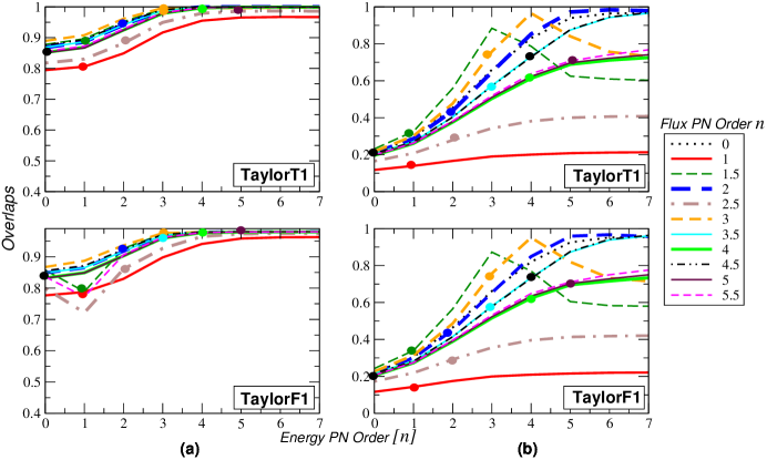
Figure 4: As in Fig. 2 except that the signal corresponds to a $(1M_{\odot},100M_{\odot})$ binary.

II.3 Comparison of standard and complete adiabatic approximants

We present the results of our study in the test mass limit in four parts. In the first part we discuss our conclusions on the mathematical problem of the closeness of the standard adiabatic and complete adiabatic template families with the family of exact waveforms in the adiabatic approximation. In the next part we exhibit our results in the case of the initial LIGO detector. In the third part we compare the relative importance of improving the accuracy of the energy and flux functions. Finally, in the fourth part we compare the total number of GW cycles and the number of useful cycles accumulated by various standard adiabatic and complete adiabatic approximants.

II.3.1 White-noise case

Table 1: Effectualness of standard adiabatic $T(E_{[n]},{\cal F}_{n})$ and complete adiabatic $T(E_{[n+2.5]},{\cal F}_{n})$ templates in the test mass limit. Overlaps are calculated assuming a flat spectrum for the detector noise (white-noise).

	$(1M_{\odot},10M_{\odot})$				$(1M_{\odot},50M_{\odot})$				$(1M_{\odot},100M_{\odot})$
	TaylorT1		TaylorF1		TaylorT1		TaylorF1		TaylorT1		TaylorF1
Order ($n$)	S	C	S	C	S	C	S	C	S	C	S	C
0PN	0.6250	0.8980	0.6212	0.8949	0.5809	0.9726	0.5917	0.9644	0.8515	0.9231	0.8318	0.9017
1PN	0.4816	0.5119	0.4801	0.5086	0.4913	0.9107	0.4841	0.5871	0.8059	0.9169	0.7874	0.8980
1.5PN	0.9562	0.9826	0.9448	0.9592	0.9466	0.9832	0.9370	0.9785	0.8963	0.9981	0.7888	0.9788
2PN	0.9685	0.9901	0.9514	0.9624	0.9784	0.9917	0.9719	0.9872	0.9420	0.9993	0.9178	0.9785
2.5PN	0.9362	0.9924	0.9298	0.9602	0.7684	0.9833	0.7326	0.9772	0.8819	0.9858	0.8610	0.9730
3PN	0.9971	0.9991	0.9677	0.9713	0.9861	0.9946	0.9821	0.9886	0.9965	0.9959	0.9756	0.9792
3.5PN	0.9913	0.9996	0.9636	0.9688	0.9902	0.9994	0.9858	0.9914	0.9885	1.0000	0.9690	0.9800
4PN	0.9937	0.9973	0.9643	0.9663	0.9975	0.9996	0.9903	0.9914	0.9968	0.9992	0.9769	0.9795
4.5PN	0.9980	0.9999	0.9671	0.9690	0.9967	1.0000	0.9902	0.9913	0.9996	1.0000	0.9787	0.9801
5PN	0.9968	0.9979	0.9661	0.9667	0.9994	0.9994	0.9913	0.9914	0.9992	0.9991	0.9790	0.9797

Table 2: Faithfulness of standard adiabatic $T(E_{[n]},{\cal F}_{n})$ and complete adiabatic $T(E_{[n+2.5]},{\cal F}_{n})$ templates in the test mass limit. Overlaps are calculated assuming a flat spectrum for the detector noise (white-noise).

	$(1M_{\odot},10M_{\odot})$				$(1M_{\odot},50M_{\odot})$				$(1M_{\odot},100M_{\odot})$
	TaylorT1		TaylorF1		TaylorT1		TaylorF1		TaylorT1		TaylorF1
Order ($n$)	S	C	S	C	S	C	S	C	S	C	S	C
0PN	0.6124	0.1475	0.6088	0.1446	0.2045	0.4683	0.2104	0.4750	0.2098	0.4534	0.2208	0.4641
1PN	0.1322	0.1433	0.1350	0.1461	0.1182	0.1446	0.1236	0.1508	0.1395	0.1901	0.1432	0.1994
1.5PN	0.5227	0.4005	0.5241	0.3967	0.3444	0.3947	0.3505	0.3866	0.3260	0.7869	0.3399	0.7700
2PN	0.7687	0.5707	0.7680	0.5689	0.5518	0.6871	0.5535	0.6827	0.4377	0.8528	0.4506	0.8486
2.5PN	0.4735	0.5268	0.4748	0.5278	0.2874	0.3561	0.2933	0.3625	0.2787	0.4001	0.2918	0.4133
3PN	0.8629	0.8165	0.8932	0.8277	0.9420	0.6317	0.9334	0.6222	0.7579	0.8407	0.7570	0.8194
3.5PN	0.9309	0.9979	0.9194	0.9609	0.6689	0.9681	0.6695	0.9632	0.5740	0.9425	0.5805	0.9383
4PN	0.9174	0.9303	0.9087	0.9176	0.6693	0.7227	0.6701	0.7230	0.6129	0.7112	0.6236	0.7159
4.5PN	0.9525	0.9744	0.9330	0.9415	0.7829	0.9242	0.7827	0.9229	0.7286	0.9689	0.7308	0.9632
5PN	0.9370	0.9392	0.9225	0.9241	0.7275	0.7417	0.7276	0.7420	0.6972	0.7409	0.7027	0.7500

First, we explore the general question of the closeness of the standard adiabatic and complete adiabatic templates to the exact waveform assuming flat power spectral density for the detector noise. Figs. 2–4 show the effectualness and faithfulness of various PN templates for three archetypical binaries with component masses ($1M_{\odot},10M_{\odot}$), ($1M_{\odot},50M_{\odot}$) and ($1M_{\odot},100M_{\odot}$), respectively .

The central result of this study is that complete adiabatic approximants bring about a remarkable improvement in the effectualness for all systems at low PN orders ($<$ 3PN). The complete adiabatic approximants converge to the adiabatic exact waveform at lower PN orders than the standard adiabatic approximants. This indicates that at these orders general relativistic corrections to the conservative dynamics of the binary are quite important contrary to the assumption employed in the standard post-Newtonian treatment of the phasing formula. On the other hand, the difference in effectualness between the standard and complete adiabatic approximants at orders greater than 3PN is very small. Thus, if we have a sufficiently accurate (order $\geq$ 3PN) T-approximant of the flux function, the standard adiabatic approximation is nearly as good as the complete adiabatic approximation for construction of effectual templates. But at all orders the standard adiabatic approximation provides a lower bound to the complete adiabatic approximation for the construction of effectual templates.

The faithfulness of both the approximants fluctuates as we go from one PN order to the next and is generally much smaller than our target value of 0.965. The fluctuation continues all the way up to 5PN order reflecting the oscillatory approach of the flux function to the exact flux function at different PN orders. It is again interesting to note that complete adiabatic approximants are generally more faithful than the standard adiabatic approximants. It is certainly worth exploring, in a future study, the anomalous cases where it performs worse than the standard.

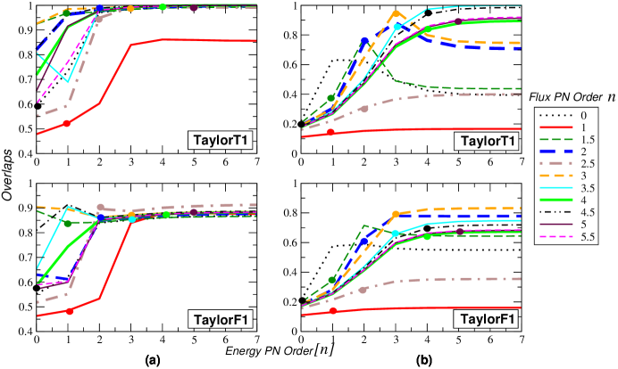
Figure 5: Effectualness (left panels) and faithfulness (right panels) of various test mass TaylorT1 and TaylorF1 templates in detecting a signal from a $(1M_{\odot},10M_{\odot})$, calculated for the initial LIGO noise PSD. Different lines in the panels correspond to different orders of the flux function. Each line shows how the overlaps are evolving as a function of the accuracy of the energy function. Standard adiabatic approximants $T(E_{[n]},{\cal F}_{n})$ are marked with thick dots.

II.3.2 Initial LIGO noise spectrum

Having addressed the general question concerning the closeness of standard adiabatic and complete adiabatic templates to the exact waveforms, we now compare the overlaps in the specific case of the initial LIGO detector. The effectualness and faithfulness of various test mass PN templates for the $(1M_{\odot},10M_{\odot})$ binary and $(1M_{\odot},50M_{\odot})$ binary are plotted in Fig. 5 and Fig. 6, respectively, and are shown in Tables LABEL:table:Effectualness1-SC-IL, LABEL:table:Effectualness2-SC-IL and LABEL:table:Faithfulness-SC-IL. As in the case of white-noise, here too we see that standard adiabatic approximants of order less than 3PN have considerably lower overlaps than the corresponding complete adiabatic approximants and the difference in overlaps between standard adiabatic and complete adiabatic approximants of order $\geq$ 3PN is very small. Thus, as in the white-noise case, if we have a sufficiently accurate (order $\geq$ 3PN) T-approximant of the flux function, the standard adiabatic approximation is nearly as good as the complete adiabatic approximation for the construction of effectual templates. Unlike in the white-noise case, for the initial LIGO noise spectrum the plots and Table LABEL:table:Faithfulness-SC-IL indicate that the faithfulness of PN templates greatly improves in a complete adiabatic treatment, for all orders studied.

We also calculate the bias in the estimation of parameters while maximizing the overlaps over the intrinsic parameters of the binary. The (percentage) bias in the estimation of the parameter $p$ is defined as

$$\sigma_{p}\equiv\frac{|p_{\rm max}-p|}{p}\times 100\,,$$ (10)

where $p_{\rm max}$ is the value of the parameter $p$ which gives the maximum overlap. Along with the maximized overlaps (effectualness), the bias in the estimation of the parameters $m$ and $\eta$ are also quoted in Tables LABEL:table:Effectualness1-SC-IL, LABEL:table:Effectualness2-SC-IL. It can be seen that at lower PN orders (order $<$ 3PN) the complete adiabatic approximants show significantly lower biases. Even at higher PN orders complete adiabatic approximants are generally less-biased than the corresponding standard adiabatic approximants.

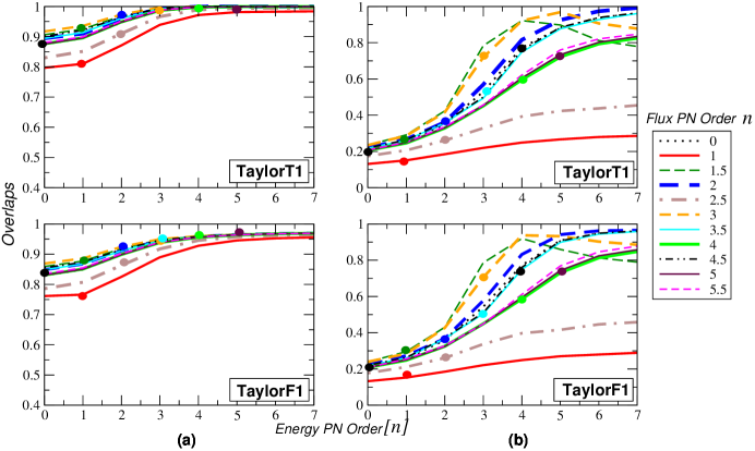
Figure 6: As in Fig. 5 except that the signal corresponds to a $(1M_{\odot},50M_{\odot})$ binary.

Table 3: Effectualness of standard adiabatic $T(E_{[n]},{\cal F}_{n})$ and complete adiabatic $T(E_{[n+2.5]},{\cal F}_{n})$ approximants in the test mass limit. Overlaps are calculated for the initial LIGO noise spectrum. Percentage biases $\sigma_{m}$ and $\sigma_{\eta}$ in determining parameters $m$ and $\eta$ are given in brackets.

	$(1M_{\odot},10M_{\odot})$
	TaylorT1			TaylorF1
Order ($n$)	S		C	S		C
0PN	0.5910 (12, 5.7)		0.9707 (36, 45)	0.5527 (31, 28)		0.8395 (48, 53)
1PN	0.5232 (22, 105)		0.8397 (125, 69)	0.4847 (18, 9.7)		0.8393 (147, 74)
1.5PN	0.9688 (52, 51)		0.9887 (8.3, 15)	0.8398 (61, 57)		0.8606 (4.7, 10)
2PN	0.9781 (18, 25)		0.9942 (0.4, 0.6)	0.8485 (32, 40)		0.8693 (15, 22)
2.5PN	0.9490 (96, 68)		0.9923 (26, 32)	0.8963 (123, 75)		0.9071 (49, 50)
3PN	0.9942 (0.3, 1.1)		0.9989 (3.7, 6.2)	0.8713 (16, 23)		0.8822 (12, 18)
3.5PN	0.9940 (6.9, 11)		0.9998 (0.6, 1.4)	0.8685 (23, 31)		0.8834 (17, 25)
4PN	0.9974 (6.2, 11)		0.9996 (3.9, 6.9)	0.8746 (23, 30)		0.8817 (21, 28)
4.5PN	0.9988 (3.3, 5.5)		1.0000 (0.8, 1.6)	0.8795 (19, 27)		0.8868 (18, 26)
5PN	0.9992 (4.0, 6.9)		0.9997 (3.5, 5.7)	0.8792 (21, 29)		0.8825 (20, 28)

Table 4: Same as Table  LABEL:table:Effectualness1-SC-IL except that the values corresponds to the $(1M_{\odot},50M_{\odot})$ binary.

	$(1M_{\odot},50M_{\odot})$
	TaylorT1			TaylorF1
Order ($n$)	S		C	S		C
0PN	0.8748 (24, 29)		0.9471 (19, 14)	0.8294 (21, 34)		0.8974 (17, 13)
1PN	0.8101 (28, 104)		0.9392 (19, 40)	0.7662 (23, 116)		0.8898 (18, 43)
1.5PN	0.9254 (21, 4.1)		0.9996 (6.7, 20)	0.8772 (18, 0.2)		0.9590 (6.4, 20)
2PN	0.9610 (18, 16)		0.9993 (7.5, 16)	0.9113 (16, 14)		0.9583 (7.7, 17)
2.5PN	0.9104 (21, 6.9)		0.9940 (8.3, 0.7)	0.8630 (19, 8.7)		0.9574 (9.1, 1.9)
3PN	0.9968 (11, 21)		0.9992 (2.6, 10)	0.9500 (11, 21)		0.9648 (2.7, 11)
3.5PN	0.9923 (13, 19)		0.9997 (2.4, 5.2)	0.9445 (12, 18)		0.9679 (2.8, 6.5)
4PN	0.9979 (8.8, 13)		0.9995 (3.5, 4.3)	0.9560 (8.9, 14)		0.9672 (3.9, 5.6)
4.5PN	0.9995 (7.1, 14)		1.0000 (0.9, 1.9)	0.9590 (7.0, 14)		0.9698 (1.5, 3.4)
5PN	0.9994 (5.2, 7.7)		0.9990 (2.6, 2.4)	0.9634 (5.9, 10)		0.9690 (3.4, 5.1)

Table 5: Faithfulness of standard adiabatic $T(E_{[n]},{\cal F}_{n})$ and complete adiabatic $T(E_{[n+2.5]},{\cal F}_{n})$ templates in the test mass limit. Overlaps are calculated for the initial LIGO noise spectrum.

	$(1M_{\odot},10M_{\odot})$				$(1M_{\odot},50M_{\odot})$
	TaylorT1		TaylorF1		TaylorT1		TaylorF1
Order ($n$)	S	C	S	C	S	C	S	C
0PN	0.2186	0.6272	0.2108	0.5879	0.2134	0.3498	0.2145	0.3593
1PN	0.1342	0.1615	0.1308	0.1563	0.1511	0.2196	0.1527	0.2210
1.5PN	0.3788	0.4492	0.3449	0.6471	0.2915	0.9223	0.2956	0.9195
2PN	0.7449	0.7633	0.6279	0.7782	0.3613	0.8157	0.3674	0.8318
2.5PN	0.3115	0.3970	0.2905	0.3532	0.2608	0.4233	0.2606	0.4161
3PN	0.9633	0.7566	0.7913	0.8297	0.7194	0.9686	0.7057	0.9323
3.5PN	0.8385	0.9984	0.6582	0.7464	0.4941	0.9273	0.5046	0.9442
4PN	0.8356	0.8909	0.6527	0.6725	0.5960	0.7934	0.5864	0.8131
4.5PN	0.9395	0.9851	0.6967	0.7195	0.7594	0.9644	0.7605	0.9614
5PN	0.8960	0.9129	0.6770	0.6821	0.7344	0.8350	0.7432	0.8579

II.3.3 Accuracy of energy function Vs. flux function

In most of the cases, TaylorT1 and TaylorF1 templates show trends of smoothly increasing overlaps as the accuracy of the energy function is increased keeping the accuracy of the flux function constant. This is because the T-approximants of the energy function smoothly converge to the exact energy as we go to higher orders (see Fig. 1$a$). On the other hand, if we improve the accuracy of the flux function for a fixed order of energy, the overlaps do not show such a smoothly converging behavior. This can be understood in terms of the oscillatory nature of the T-approximants of the flux function. For example, templates constructed from 1PN and 2.5PN flux functions can be seen to have considerably lower overlaps than the other ones. This is because of the poor ability of the 1PN and 2.5PN T-approximants to mimic the behavior of the exact flux function (see Fig. 1$b$). This inadequacy of the 1PN and 2.5PN T-approximants is prevalent in both test mass and comparable mass cases. Hence it is not a good strategy to use the T-approximants at these orders for the construction of templates. On the other hand, 3.5PN and 4.5PN T-approximants are greatly successful in following the exact flux function in the test mass case, and consequently lead to larger overlaps.

We have found that in the test mass case if we improve the accuracy of energy function from 3PN to 4PN, keeping the flux function at order 3PN, the increase in effectualness (respectively, faithfulness) is $\simeq 0.36\%$ $(-16\%)$. The same improvement in the energy function for the 3.5PN flux will produce an increase of $\simeq 0.36\%$ $(13\%)$. On the other hand, if we improve the accuracy of flux function from 3.5PN to 4PN, keeping the energy function at order 3PN, the increase in effectualness (respectively, faithfulness) is $\simeq-0.17\%$ $(-12\%)$. The values quoted are calculated using the TaylorT1 method for the ($1M_{\odot},\,10M_{\odot})$ binary for the initial LIGO noise PSD. The effectualness trends are similar in the case of the $(1M_{\odot},\,50M_{\odot})$ binary also. If the comparable mass case is qualitatively similar to the test mass case, this should imply that neither the improvement in the accuracy of the energy function from 3PN to 4PN nor the improvement in the accuracy of the flux function from 3.5PN to 4PN will produce significant improvement in the effectualness in the comparable mass case. The trends in the faithfulness are very different for different binaries so that it is hard to make any statement about the improvement in faithfulness.

II.3.4 Number of gravitational wave cycles

The number of GW cycles accumulated by a template is defined as dis02

$${\cal N}_{\rm tot}\equiv\frac{1}{2\pi}(\varphi_{\rm lso}-\varphi_{\rm low})=\int_{F_{\rm low}}^{F{\rm lso}}dF\frac{N(F)}{F}\,,$$ (11)

where $\varphi_{\rm lso}$ and $\varphi_{\rm low}$ are the GW phases corresponding to the last stable orbit and the low frequency cut-off, respectively, and $N(F)\equiv F^{2}/\dot{F}$ is the instantaneous number of cycles spent near some instantaneous frequency $F$ (as usual, $\dot{F}$ is the time derivative of $F$). However, it has been noticed that dis02 , the large number ${\cal N}_{\rm tot}$ is not significant because the only really useful cycles are those that contribute most to the signal-to-noise ratio (SNR). The number of useful cycles is defined as dis02

$${\cal N}_{\rm useful}\equiv\left(\int_{F_{\rm low}}^{F{\rm lso}}\frac{df}{f}w(f)N(f)\right)\left(\int_{F_{\rm low}}^{F{\rm lso}}\frac{df}{f}w(f)\right)^{-1},$$ (12)

where $w(f)\equiv a^{2}(f)/h^{2}_{n}(f)$. If $S_{n}(f)$ is the two-sided PSD of the detector noise, $h_{n}(f)$ is defined by $h_{n}^{2}(f)\equiv fS_{n}(f)$, while $a(f)$ is defined by $|H(f)|\simeq a(t_{f})/[{\dot{F}(t_{f})}]^{1/2}$ where $H(f)$ is the Fourier transform of the time-domain waveform $h(t)$ (See Eqs.(2) and (3)) and $t_{f}$ is the time when the instantaneous frequency $F(t)$ reaches the value $f$ of the Fourier variable.

The total numbers of GW cycles accumulated by various standard adiabatic $T(E_{[n]},{\cal F}_{n})$ and complete adiabatic $T(E_{[n+2.5]},{\cal F}_{n})$ approximants in the test mass limit are tabulated in Table LABEL:table:cycles20 along with the number of useful cycles calculated for the initial LIGO noise PSD. We use Eq.(4) to calculate $\dot{F}$ and numerically evaluate the integrals in Eq.(12) to compute the number of useful cycles. In order to compute the total number of cycles, we numerically evaluate the integral in Eq.(11)

It can be seen that all complete adiabatic approximants accumulate fewer number of (total and useful) cycles than the corresponding standard adiabatic approximants. This is because the additional conservative terms in the complete adiabatic approximants add extra acceleration to the test mass which, in the presence of radiation reaction, would mean that the test body has to coalesce faster, and therefore such templates accumulate fewer number of cycles. Notably enough, approximants (like 3PN and 4.5PN) producing the highest overlaps with the exact waveform, accumulate the closest number of cycles as accumulated by the exact waveform. This is indicative that the phase evolution of these approximants is closer to that of the exact waveform. On the other hand, the fractional absolute difference in the number of cycles of the approximants producing the lowest overlaps (like 0PN, 1PN and 2.5PN) as compared to the exact waveform is the greatest, which indicates that these templates follow a completely different phase evolution.

In order to illustrate the correlation between the number of (total/useful) cycles accumulated by an approximant and its overlap with the exact waveform, we introduce a quantity $\delta{\cal N}_{n}=\frac{|{\cal N}_{n}-{\cal N}_{\rm exact}|}{{\cal N}_{\rm exact}}$ which is the fractional absolute difference between the number of (total/useful) cycles accumulated by a template and the exact waveform. Here ${\cal N}_{n}$ and ${\cal N}_{\rm exact}$ are the number of (total/useful) cycles accumulated by the $n$PN approximant and exact waveform, respectively. In Fig. 7, we plot $\delta{\cal N}_{n}$ of various standard adiabatic and complete adiabatic approximants against the corresponding overlaps in the case of a $(1M_{\odot},10M_{\odot})$ binary.

The following points may be noted while comparing the results quoted here for the number of cycles with those of other works, e.g. Refs. MSSTT ; BFIJ02 ; AISS . As emphasized in Ref. dis03 one can get very different results for the phasing depending on whether one consistently re-expands the constituent energy and flux functions or evaluates them without re-expansion. In the computation of the number of useful cycles different authors treat the function ${\dot{F}}$ differently, some re-expand and others do not, leading to differences in the results. The other important feature we would like to comment upon is a result that appears, at first, very counter-intuitive. It is the fact that in some cases the number of useful GW cycles is greater than the total number of GW cycles! A closer examination reveals that while for most cases of interest this does not happen, in principle its occurrence is determined by the ratio $f_{\rm r}\equiv F_{\rm low}/F_{\rm lso}$. To understand this in more detail let us consider the ratio ${\cal N}_{\rm r}$ of the number of useful cycles to the total number of cycles in the case of white-noise (in a frequency band $F_{\rm low}$ to $F_{\rm lso}$) for which

$${\cal N}_{\rm r}\equiv\frac{{\cal N}_{\rm useful}}{{\cal N}_{\rm tot}}=\frac{5}{12}f_{\rm r}^{1/3}\frac{1-f_{\rm r}^{4/3}}{1-f_{\rm r}^{1/3}}\,.$$ (13)

For $f_{\rm r}\ll 1$, ${\cal N}_{\rm r}<1$. However, as $f_{\rm r}$ increases to about $f_{\rm r}=0.52,$ ${\cal N}_{\rm r}$ transits from being less than one to becoming greater than one! Essentially this arises due to the details of the scalings of the various quantities involved and the point of transition depends on the PN order and the precise form of the noise PSD. For $f_{\rm r}\simeq 1$, the calculation of useful cycles does not make much physical sense. This explains the absence of ${\cal N}_{\rm useful}$ results for the $(1M_{\odot},100M_{\odot})$ binary in Table LABEL:table:cycles20.

Table 6: Number of GW cycles accumulated by various standard adiabatic $T(E_{[n]},{\cal F}_{n})$ and complete adiabatic $T(E_{[n+2.5]},{\cal F}_{n})$ approximants in the test mass limit. The number of useful cycles calculated for the initial LIGO noise PSD is also shown in brackets. We choose a low frequency cut-off of 40Hz.

	$(1M_{\odot},10M_{\odot})$			$(1M_{\odot},50M_{\odot})$			$(1M_{\odot},100M_{\odot})$
Order ($n$)	S		C	S		C	S		C
0PN	481 (92.3)		424 (74.6)	118 (110)		77.8 (64.4)	13.6		6.7
1PN	560 (117)		526 (102)	180 (186)		124 (104)	25.7		10.6
1.5PN	457 (81.7)		433 (71.8)	88.8 (76.3)		58.5 (38.2)	8.4		2.3
2PN	447 (77.7)		440 (74.0)	77.0 (61.8)		62.5 (41.5)	6.1		2.6
2.5PN	464 (84.5)		454 (79.6)	96.8 (85.5)		74.5 (50.5)	9.7		2.9
3PN	442 (74.7)		440 (73.3)	64.5 (45.2)		58.1 (35.5)	3.4		1.6
3.5PN	445 (76.1)		442 (74.5)	68.7 (49.7)		60.6 (36.8)	4.0		1.4
4PN	445 (75.8)		443 (75.2)	66.4 (45.1)		62.9 (39.0)	2.9		1.6
4.5PN	443 (75.1)		442 (74.5)	63.7 (42.0)		60.0 (35.6)	2.5		1.2
5PN	444 (75.3)		443 (75.0)	63.8 (40.9)		62.2 (37.8)	2.1		1.4
Exact	442 (74.1)			59.1 (34.3)			0.9

Figure 7: The fractional absolute difference $\delta{\cal N}_{n}$ between the number of cycles accumulated by various approximants and the exact waveform, plotted against the corresponding overlaps. Standard adiabatic $T(E_{[n]},{\cal F}_{n})$ approximants are marked with lighter markers and complete adiabatic $T(E_{[n+2.5]},{\cal F}_{n})$ approximants are marked with darker markers. Top panels show $\delta{\cal N}_{n}$ for the total number of cycles and bottom panels show $\delta{\cal N}_{n}$ for the number of useful cycles. The number of useful cycles are calculated for the initial LIGO noise PSD and the low frequency cut-off is chosen to be 40Hz. The plotted results are for a $(1M_{\odot},10M_{\odot})$ binary.

III Non-adiabatic models

Before introducing new non-adiabatic models in this section, let us recapitulate our point of view in summary. Contrary to the standard adiabatic approximant which is constructed from consistent PN expansions of the energy and flux functions to the same relative PN order, we considered a new complete adiabatic approximant (still based on PN expansions of the energy and flux functions but of different PN orders) but consistent with a complete PN acceleration. Viewed in terms of the acceleration terms they include, the standard adiabatic approximation is inconsistent by neglect of some intermediate PN order terms in the acceleration. The complete adiabatic approximation on the other hand is constructed to consistently include all the relevant PN acceleration terms neglected in the associated standard approximant. These models were a prelude to phasing models constructed from the dynamical equations of motion considered in this section. However, we have worked solely within the adiabatic approximation. It is then pertinent to ask whether one can construct natural non-adiabatic extensions of both the standard and complete adiabatic approximants. And if so, how do their performance compare? Indeed, the work of Buonanno and Damour bd00 within the effective one-body approach to the dynamics did find differences between the adiabatic and non-adiabatic solutions. In this Section we investigate whether it is possible to introduce non-adiabatic formulations of the standard and complete approximants considered in the previous Section.

The Lagrangian models studied by Buonanno, Chen and Vallisneri BCV02 seem to be the natural candidates for the purpose since they are specified by the acceleration experienced by the binary system. The Lagrangian models considered in Ref. BCV02 can be thought of as the standard non-adiabatic approximants, since, following standard choices, they lead to gaps in the post-Newtonian expansion of the acceleration. Generalizing these Lagrangian models so that there are no missing PN terms, or gaps, in the acceleration we can construct the complete non-adiabatic approximants. With a non-adiabatic variant of the standard and complete approximants we can then compare their relative performances. However, we will be limited in this investigation because of two reasons: Firstly, the Lagrangian models are available only up to 3.5PN order, and higher order PN accelerations are as yet unavailable. Secondly, the only exact waveform we have, has however been constructed only in the adiabatic approximation. Even in the test mass limit, the exact waveform is not known beyond the adiabatic approximation. Due to lack of anything better, we continue to use the exact waveform in the adiabatic approximation to measure the effectualness and faithfulness of the non-adiabatic approximants.

Thus to obtain non-adiabatic approximants, the signal is constructed by integrating the equations of motion directly using a Lagrangian formalism. The equations are schematically written as:

$$\frac{d\mathbf{x}}{dt}=\mathbf{v},\ \ \ \ \frac{d\mathbf{v}}{dt}=\mathbf{a}$$ (14)

For the complete non-adiabatic model of order $n$, all terms in the PN expansion for acceleration are retained up to order $n+2.5$ without any gaps. For the standard non-adiabatic models, on the other hand, only terms in the acceleration consistent with the treatment of standard phasing are retained in the acceleration, resulting in gaps in the acceleration corresponding to intermediate PN terms neglected in the treatment. E.g. for $n=0$ the standard non-adiabatic approximation includes only the $\mathbf{a}_{\rm N}$ and $\mathbf{a}_{\rm 2.5PN}$ while the complete non-adiabatic approximation would include in addition the $\mathbf{a}_{\rm 1PN}$ and $\mathbf{a}_{\rm 2PN}$. Given the current status of knowledge of the two-body equations of motion, we have only two complete non-adiabatic approximants, at 0PN and 1PN retaining all acceleration terms up to 2.5PN and 3.5PN, respectively. The associated 0PN (1PN) standard non-adiabatic approximation retains acceleration terms corresponding to 0PN and 2.5PN (0PN, 1PN, 2.5PN and 3.5PN).

The explicit terms for accelerations for each order are given as follows BCV02 ; BI03 ; MoraWill

$$\mathbf{a}_{\rm{N}} = -\frac{M}{r^{2}}\mathbf{\hat{n}},$$ (15)

$$\mathbf{a}_{\rm{1PN}} = -\frac{M}{r^{2}}\left\{\mathbf{\hat{n}}\left[(1+3\eta)v^{2}-2(2+\eta)\frac{M}{r}-\frac{3}{2}\eta\dot{r}^{2}\right]-2(2-\eta)\dot{r}\mathbf{v}\right\},$$ (16)

$$\mathbf{a}_{\rm{2PN}} = -\frac{M}{r^{2}}\left\{\mathbf{\hat{n}}\left[\frac{3}{4}(12+29\eta)\left(\frac{M}{r}\right)^{2}+\eta(3-4\eta)v^{4}+\frac{15}{8}\eta(1-3\eta)\dot{r}^{4}\right.\right.$$ (17)

$$- \left.\left.\frac{3}{2}\eta(3-4\eta)v^{2}\dot{r}^{2}-\frac{1}{2}\eta(13-4\eta)\frac{M}{r}v^{2}-(2+25\eta+2\eta^{2})\frac{M}{r}\dot{r}^{2}\right]\right.$$

$$- \left.\frac{1}{2}\dot{r}\mathbf{v}\left[\eta(15+4\eta)v^{2}-(4+41\eta+8\eta^{2})\frac{M}{r}-3\eta(3+2\eta)\dot{r}^{2}\right]\right\},$$

$$\mathbf{a}_{\rm{3PN}} = -\frac{M}{r^{2}}\left\{\mathbf{\hat{n}}\left[-\frac{35\dot{r}^{6}\eta}{16}+\frac{175\dot{r}^{6}\eta^{2}}{16}-\frac{175\dot{r}^{6}\eta^{3}}{16}+\frac{15\dot{r}^{4}\eta v^{2}}{2}-\frac{135\dot{r}^{4}\eta^{2}v^{2}}{4}+\frac{255\dot{r}^{4}\eta^{3}v^{2}}{8}\right.\right.$$ (18)

$$- \frac{15\dot{r}^{2}\eta v^{4}}{2}+\frac{237\dot{r}^{2}\eta^{2}v^{4}}{8}-\frac{45\dot{r}^{2}\eta^{3}v^{4}}{2}+\frac{11\eta v^{6}}{4}-\frac{49\eta^{2}v^{6}}{4}+13\eta^{3}v^{6}$$

$$+ \frac{M}{r}\left(79\dot{r}^{4}\eta-\frac{69\dot{r}^{4}\eta^{2}}{2}-30\dot{r}^{4}\eta^{3}-121\dot{r}^{2}\eta v^{2}+16\dot{r}^{2}\eta^{2}v^{2}+20\dot{r}^{2}\eta^{3}v^{2}\right.$$

$$+ \left.\frac{75\eta v^{4}}{4}+8\eta^{2}v^{4}-10\eta^{3}v^{4}\right)+\frac{M^{2}}{r^{2}}\left(\dot{r}^{2}+\frac{22717\dot{r}^{2}\eta}{168}+\frac{11\dot{r}^{2}\eta^{2}}{8}-7\dot{r}^{2}\eta^{3}\right.$$

$$+ \left.\frac{615\dot{r}^{2}\eta\pi^{2}}{64}-\frac{20827\eta v^{2}}{840}+\eta^{3}v^{2}-\frac{123\eta\pi^{2}v^{2}}{64}\right)$$

$$+ \left.\frac{M^{3}}{r^{3}}\left(-16-\frac{1399\eta}{12}-\frac{71\eta^{2}}{2}+\frac{41\eta\pi^{2}}{16}\right)\right]+\mathbf{v}\left[-\frac{45\dot{r}^{5}\eta}{8}+15\dot{r}^{5}\eta^{2}\right.$$

$$+ \left.\frac{15\dot{r}^{5}\eta^{3}}{4}+12\dot{r}^{3}\eta v^{2}-\frac{111\dot{r}^{3}\eta^{2}v^{2}}{4}-12\dot{r}^{3}\eta^{3}v^{2}-\frac{65\dot{r}\eta v^{4}}{8}+19\dot{r}\eta^{2}v^{4}+6\dot{r}\eta^{3}v^{4}\right.$$

$$+ \frac{M}{r}\left(\frac{329\dot{r}^{3}\eta}{6}+\frac{59\dot{r}^{3}v^{2}}{2}+18\dot{r}^{3}\eta^{3}-15\dot{r}\eta v^{2}-27\dot{r}\eta^{2}v^{2}-10\dot{r}\eta^{3}v^{2}\right)$$

$$+ \left.\left.\frac{M^{2}}{r^{2}}\left(-4\dot{r}-\frac{5849\dot{r}\eta}{840}+25\dot{r}\eta^{2}+8\dot{r}\eta^{3}-\frac{123\dot{r}\eta\pi^{2}}{32}\right)\right]\right\},$$

$$\mathbf{a}_{\rm{2.5RR}} = \frac{8}{5}\eta\frac{M^{2}}{r^{3}}\left\{\dot{r}\mathbf{\hat{n}}\left[18v^{2}+\frac{2}{3}\frac{M}{r}-25\dot{r}^{2}\right]-\mathbf{v}\left[6v^{2}-2\frac{M}{r}-15\dot{r}^{2}\right]\right\},$$ (19)

$$\mathbf{a}_{\rm{3.5RR}} = \frac{8}{5}\eta\frac{M^{2}}{r^{3}}\left\{\dot{r}\mathbf{\hat{n}}\left[\left(\frac{87}{14}-48\eta\right)v^{4}-\left(\frac{5379}{28}+\frac{136}{3}\eta\right)v^{2}\frac{M}{r}+\frac{25}{2}(1+5\eta)v^{2}\dot{r}^{2}\right.\right.$$ (20)

$$+ \left.\left(\frac{1353}{4}+133\eta\right)\dot{r}^{2}\frac{M}{r}-\frac{35}{2}(1-\eta)\dot{r}^{4}+\left(\frac{160}{7}+\frac{55}{3}\eta\right)\left(\frac{M}{r}\right)^{2}\right]$$

$$- \mathbf{v}\left[-\frac{27}{14}v^{4}-\left(\frac{4861}{84}+\frac{58}{3}\eta\right)v^{2}\frac{M}{r}+\frac{3}{2}(13-37\eta)v^{2}\dot{r}^{2}\right.$$

$$+ \left.\left.\left(\frac{2591}{12}+97\eta\right)\dot{r}^{2}\frac{M}{r}-\frac{25}{2}(1-7\eta)\dot{r}^{4}+\frac{1}{3}\left(\frac{776}{7}+55\eta\right)\left(\frac{M}{r}\right)^{2}\right]\right\},$$

where $\mathbf{\hat{n}}=\mathbf{r}/r$. In the above Eq.(18), the logarithmic terms present in $\mathbf{a}_{\rm 3PN}$ in BI03 have been transformed away by an infinitesimal gauge transformation following MoraWill .

The above equations are solved numerically to attain the dynamics of the system. Then the orbital phase $\phi(t)$ is calculated by numerically solving the equations

$$\frac{d\phi}{dt}=\omega,\,\,\,\,\,\,v^{2}=\omega^{2}r^{2}.$$ (21)

where the calculation of the orbital angular frequency $\omega$ assumes that the orbit is circular. Once we have the orbital phase, the waveform is generated using Eq.(2) since the orbital phase $\phi$ is related to the GW phase $\varphi$ by $\varphi=2\phi$.

III.1 Standard and complete non-adiabatic approximants in the test mass case

In the following we discuss the results of our study for the non-adiabatic waveforms in the test mass limit. To determine the appropriate expressions for the acceleration in the test mass case, we start with the general expression for the acceleration and set $\eta=0$ in the conservative 1PN, 2PN and 3PN terms. Since doing the same in the dissipative terms at 2.5PN and 3.5PN orders prevents the orbit from decaying, we retain terms linear in $\eta$ at these orders and set to zero terms of higher order in $\eta$. In the first part we discuss results found on the problem of the closeness of the standard and complete non-adiabatic template families with the fiducial exact waveform. In the second part we extend our results to the noise spectrum expected in initial LIGO.

III.1.1 White noise

Table 7: Effectualness of the Lagrangian templates in the test mass case for the white-noise.

	$(1M_{\odot},10M_{\odot})$		$(1M_{\odot},50M_{\odot})$		$(1M_{\odot},100M_{\odot})$
Order ($n$)	S	C	S	C	S	C
0PN	0.5521	0.4985	0.5553	0.8399	0.6775	0.7789
1PN	0.4415	0.4702	0.5760	0.8327	0.6557	0.7591

Table 8: Faithfulness of the Lagrangian templates in the test mass case for the white-noise.

	$(1M_{\odot},10M_{\odot})$		$(1M_{\odot},50M_{\odot})$		$(1M_{\odot},100M_{\odot})$
Order ($n$)	S	C	S	C	S	C
0PN	0.0450	0.0441	0.1778	0.0991	0.5959	0.1851
1PN	0.0471	0.0474	0.3195	0.1235	0.3646	0.2404

First, we explore the general question as to the closeness of the standard non-adiabatic and complete non-adiabatic templates assuming a flat power spectral density for the detector noise. Tables LABEL:table:Effectualness-LM-TM-WN and LABEL:table:Faithfulness-LM-TM-WN show the effectualness and faithfulness of Lagrangian models for the same three archetypical binaries as before: $(1M_{\odot},\,10M_{\odot})$, $(1M_{\odot},\,50M_{\odot})$ and $(1M_{\odot},\,100M_{\odot})$ binaries. At present, the results are available at too few PN orders to make statements of general trends in effectualness and faithfulness. However, the main result obtained for the adiabatic approximants seems to hold good again for the non-adiabatic approximants: the effectualness is higher for the complete non-adiabatic model as opposed to the standard non-adiabatic model. This is indicative of the fact that corrections coming from the conservative part of the dynamics (i.e. the well-known general relativistic effects at 1PN and 2PN) make an improvement of the effectualness. However, as in the adiabatic case, the faithfulness of both standard and complete non-adiabatic models is very poor. But, in sharp contrast to the adiabatic case, here it appears that the complete non-adiabatic approximation results in a decrease in the faithfulness of the templates.

III.1.2 Initial LIGO noise spectrum

Having addressed the question concerning the closeness of standard non-adiabatic and complete non-adiabatic templates to exact waveforms, we now compare the overlaps in the case of the initial LIGO detector.

Table 9: Effectualness of the Lagrangian templates in the test mass case for the initial LIGO noise PSD. Percentage biases $\sigma_{m}$ and $\sigma_{\eta}$ in determining parameters $m$ and $\eta$ are given in brackets.

	$(1M_{\odot},10M_{\odot})$		$(1M_{\odot},50M_{\odot})$
Order ($n$)	S	C	S	C
0PN	0.5848 (30, 26)	0.9496 (55, 107)	0.8741 (3.3, 9.2)	0.9835 (35, 4.2)
1PN	0.6762 (37, 49)	0.9273 (3.1, 27)	0.8530 (34, 191)	0.9784 (24, 28)

Table 10: Faithfulness of the Lagrangian templates in the test mass case for the initial LIGO noise PSD.

	$(1M_{\odot},10M_{\odot})$		$(1M_{\odot},50M_{\odot})$
Order ($n$)	S	C	S	C
0PN	0.2463	0.1216	0.5048	0.1747
1PN	0.4393	0.1823	0.3650	0.3119

Tables LABEL:LagrangianEffectualnessLIGOTest and LABEL:LagrangianFaithfulnessLIGOTest show the effectualness and faithfulness, respectively, of Lagrangian templates for the $(1M_{\odot},\,10M_{\odot})$ and $(1M_{\odot},\,50M_{\odot})$ binaries. In this case, we see the that the effectualness of the approximants gets significantly improved in the complete non-adiabatic approximation and is greater than 0.9 for all the systems studied in this paper. Faithfulness appears to be decreased by the use of complete non-adiabatic approximation (this result also is in sharp contrast with the corresponding adiabatic case where we find that the complete approximation brings about a significant improvement in the faithfulness), but again there is no indication that either standard or complete templates are reliable in extracting the parameters of the system.

IV Comparable Mass Waveforms

In the case of comparable mass binaries there is no exact template available and the best we can do is to compare the performance of the standard adiabatic and complete adiabatic templates by studying their overlaps with some plausible fiducial ‘exact’ waveform. As in the case of the test masses, here too we will consider all possible combinations of the T-approximants of the energy and flux functions, construct PN templates and calculate the overlaps of these templates with the fiducial ‘exact’ waveform. In all cases, the fiducial ‘exact’ waveform is constructed by numerically integrating the phasing formula in the time-domain (TaylorT1 approximant), and terminating the waveforms (‘exact’ and approximate) at $v_{lso}=1/\sqrt{6}$ which corresponds to $F_{\rm lso}\simeq 1570$ Hz for a $(1.4M_{\odot},\,1.4M_{\odot})$ binary and $F_{\rm lso}\simeq 220$ Hz for a $(10M_{\odot},\,10M_{\odot})$ binary . The lower frequency cut-off of the waveforms is chosen to be $F_{\rm low}=40$ Hz.

IV.1 The energy function

Unlike in the test mass limit, the energy function $E(x;\eta)$ is not known exactly in the comparable mass case but only a post-Newtonian expansion, which has been computed at present up to 3PN accuracy DJS ; BF ; DJS02 ; BDE03 ; IF .

$$E_{3PN}(x;\eta) = -\frac{1}{2}\,\eta\,x\,\left[1-\frac{1}{12}\right.\,(9+\eta)\,x-\frac{1}{8}\,\left(27-19\eta+\frac{\eta^{2}}{3}\right)\,x^{2}$$ (22)

$$+ \left(\frac{-\,675}{64}+\left(\frac{209323}{4032}-\frac{205\pi^{2}}{96}\right.\right.\left.-\frac{110\lambda}{9}\right)\eta-\frac{155}{96}\eta^{2}\left.-\frac{35}{5184}\eta^{3}\right)\,x^{3}+{\cal O}\,(x^{4})\,\bigg{]}\,,$$

where $\lambda=-1987/3080\simeq-0.6451$ DJS02 ; BDE03 ; IF ; itoh2 . The corresponding $E^{\prime}(v;\eta)$ appearing in the phasing formula reads,

$$E^{\prime}_{3PN}(v;\eta) = -\eta\,v\,\left[1-\frac{1}{6}\,\right.\,(9+\eta)\,v^{2}-\frac{3}{8}\,\left(27-19\eta+\frac{\eta^{2}}{3}\right)\,v^{4}$$ (23)

$$+ 4\left(\frac{-\,675}{64}+\left(\frac{209323}{4032}-\frac{205\pi^{2}}{96}\right.\right.\left.-\frac{110\lambda}{9}\right)\eta-\frac{155}{96}\eta^{2}\left.-\frac{35}{5184}\eta^{3}\right)\,v^{6}+{\cal O}(v^{8})\,\bigg{]}.$$

We use this expression truncated at the necessary orders to construct the various approximate templates. To compute a fiducial ‘exact’ waveform, we use the exact energy function in the test mass limit supplemented by the finite mass corrections up to 3PN in the spirit of the hybrid approximation KWW . In other words, the fiducial ‘exact’ energy $E^{\prime}(v;\eta)$ will look like

$$E^{\prime}_{\rm exact}(v;\eta) = -\eta\,v\,\left[\frac{-\,E^{\prime}_{\rm exact}(v)}{\eta\,v}-\frac{\eta}{6}\,v^{2}\right.\,-\frac{3}{8}\,\left(-19\,\eta+\frac{\eta^{2}}{3}\right)\,v^{4}$$ (24)

$$+ 4\left(\left(\frac{209323}{4032}-\frac{205\,\pi^{2}}{96}\right.\right.\left.-\frac{110\lambda}{9}\right)\eta-\frac{155}{96}\eta^{2}\left.\left.-\frac{35}{5184}\eta^{3}\right)\,v^{6}\,\right]$$

where $E^{\prime}_{\rm exact}(v)$ is the v-derivative of the exact energy function in the test mass limit given by Eq. (6). The T-approximants of the energy function $E^{\prime}_{\rm T}(v;\eta)$ as well as the fiducial exact energy $E^{\prime}_{\rm exact}(v;\eta)$ are plotted in Fig. 8$a$. The $v_{\rm lso}$ corresponding to the fiducial ‘exact’ energy function can be determined by solving $E^{\prime}_{\rm exact}(v;\eta)=0$. This will yield a value $v_{\rm lso}^{\rm 3PN-hybrid}\simeq 0.4294$ against the $v_{\rm lso}\simeq 0.4082$ in the test-mass case (more precisely it is the $v_{\rm MECO}$ BCV02 ). If the $\eta$-corrections are included only up to 2PN instead of 3PN, $v_{\rm lso}^{\rm 2PN-hybrid}\simeq 0.4113$. It is worth pointing that $v_{\rm lso}^{\rm 2PN-Pade}\simeq 0.4456$ dis01 and it is not unreasonable to expect that, with 3PN $\eta$-corrections the differences between various different ways of determining the lso converge. (For the purposes of our analysis, we have checked that there is no drastic change in our conclusions due to these differences and hence we use uniformly the value $v_{\rm lso}=0.4082$).

IV.2 The flux function

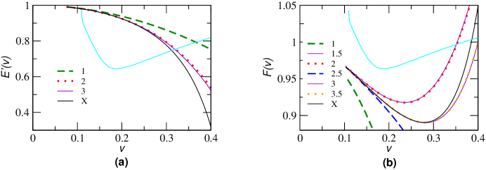
Figure 8: Various T-approximants of Newton-normalized ($v$-derivative of) energy function $E^{\prime}_{\rm T}(v)/E^{\prime}_{\rm N}(v)$ (left) and flux function ${\cal F}_{\rm T}(v)/{\cal F}_{\rm N}(v)$ (right) in the comparable mass case, along with the corresponding fiducial ‘exact’ functions (denoted by $X$). Also plotted is the amplitude spectral density (per $\sqrt{\rm Hz}$) of initial LIGO noise in arbitrary units.

The flux function in the case of comparable masses has been calculated up to 3.5PN accuracy BDIWW ; BDI ; WW ; BIWW ; B96 ; BIJ02 ; BFIJ02 , and is given by:

$${\cal F}(v;\eta)=\frac{32}{5}\eta^{2}v^{10}\left[\sum_{k=0}^{7}A_{k}(\eta)v^{k}+B_{6}(\eta)v^{6}\ln v+{\cal O}\,(v^{8})\,\right],$$ (25)

where

$$A_{0}(\eta) = 1,\ \ A_{1}(\eta)=0,\ \ A_{2}(\eta)=-\frac{1247}{336}-\frac{35}{12}\,\eta,\ \ A_{3}(\eta)=4\pi,$$

$$A_{4}(\eta) = -\frac{44711}{9072}+\frac{9271}{504}\,\eta+\frac{65}{18}\,\eta^{2},$$ (26)

$$A_{5}(\eta) = -\left(\frac{8191}{672}+\frac{583}{24}\,\eta\right)\,\pi,$$

$$A_{6}(\eta) = \frac{6643739519}{69854400}+\frac{16\pi^{2}}{3}-\frac{1712}{105}\gamma+\left(-\frac{11497453}{272160}+\frac{41\pi^{2}}{48}+\frac{176\lambda}{9}-\frac{88\Theta}{3}\right)\eta$$

$$- \frac{94403}{3024}\eta^{2}-\frac{775}{324}\eta^{3}-\frac{1712}{105}\,{\rm ln}\,4,$$

$$A_{7}(\eta) = \left(-\frac{16285}{504}+\frac{214745}{1728}\eta+\frac{193385}{3024}\eta^{2}\right)\,\pi,$$ (27)

$$B_{6}(\eta) = -\frac{1712}{105},$$ (28)

and the value of $\Theta$ has been recently calculated to be $-11831/9240\simeq-1.28$ BDEI by dimensional regularization.

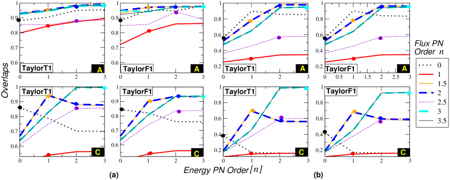
Figure 9: Effectualness (Fig. $a$) and Faithfulness (Fig. $b$) of various TaylorT1 and TaylorF1 templates in the comparable mass case for the initial LIGO noise spectrum. Different lines in the panels correspond to different orders of the flux function. Each line shows how the overlaps are evolving as a function of the accuracy of the energy function. Standard adiabatic approximants $T(E_{[n]},{\cal F}_{n})$ are marked with thick dots. Label A represents the $(10M_{\odot},\,10M_{\odot})$ binary and label C represents the $(1.4M_{\odot},\,1.4M_{\odot})$ binary.

To construct our fiducial ‘exact’ waveform, we will use the energy function given by Eq. (24) and the flux function

$${\cal F}_{\rm exact}(v;\eta) = \frac{32}{5}\eta^{2}v^{10}\left[{\cal F}_{\rm exact}(v)-\sum_{k=0}^{7}\left(A_{k}v^{k}\right.\right.\left.+B_{6}v^{6}\ln v\right)+\left.\sum_{k=0}^{7}\left(A_{k}(\eta)v^{k}+B_{6}(\eta)v^{6}\ln v\right)\right],$$ (29)

where ${\cal F}_{\rm exact}(v)$ is the Newton-normalized (numerical) exact flux in the test-mass limit. The expansion coefficients $A_{k}$’s and $B_{6}$ refer to the test-mass case and $A_{k}(\eta)$’s and $B_{6}(\eta)$ refer to the comparable mass case. The exact flux function is thus constructed by superposing all that we know in the test mass case from perturbation methods and the two body case by post-Newtonian methods. It supplements the exact flux function in the test body limit by all the $\eta$-dependent corrections known up to 3.5PN order in the comparable mass case. The T-approximants of the flux function ${\cal F}_{\rm T}(v;\eta)$ and the fiducial exact flux ${\cal F}_{\rm exact}(v;\eta)$ are plotted in Fig. 8$b$.

IV.3 Comparable mass results in the adiabatic approximation

The effectualness and faithfulness of various PN templates in the case of comparable mass binaries are plotted in Fig. 9$a$ and Fig. 9$b$, respectively, and are tabulated in Tables LABEL:table:Effectualness1-SC-CM-IL, LABEL:table:Effectualness2-SC-CM-IL and LABEL:table:Faithfulness-SC-CM-WN. The overlaps of the fiducial ‘exact’ waveform are calculated with the TaylorT1 and TaylorF1 approximants using the initial LIGO noise spectrum. Different lines in the panels of Fig. 9 correspond to different PN orders of the flux function. Let us note that in the case of comparable mass binaries the complete adiabatic approximants can be calculated, at present, at most up to 1PN order. From the Tables LABEL:table:Effectualness1-SC-CM-IL, LABEL:table:Effectualness2-SC-CM-IL and LABEL:table:Faithfulness-SC-CM-WN one can see that the complete adiabatic approximation generally improves the effectualness of the templates at 0PN and 1PN orders. But, as far as faithfulness is concerned, it is hard to conclude that one approximation is better than the other at these PN orders.

Even though complete adiabatic approximants are not calculated for higher PN orders, the general conclusion one can make from Fig. 9 is that the complete adiabatic approximation of the phasing will not result in a significant improvement in overlaps if we have a flux function of order $\geq$ 1.5PN. We, thus, conclude that, provided we have a sufficiently accurate (order $\geq$ 1.5PN) T-approximant of the flux function, the standard adiabatic approximation provides a good lower bound to the complete adiabatic approximation for the construction of both effectual and faithful templates in the case of comparable mass binaries. It should be kept in mind that unlike the test mass case where the exact energy and flux functions are known leading to an exact waveform in the adiabatic approximation, in the comparable mass case we are only talking about fiducial energy and flux functions constructed from what is known. Probably, the fiducial waveform in this case has much less to do with the exact waveform predicted by general relativity.

Tables LABEL:table:Effectualness1-SC-CM-IL and LABEL:table:Effectualness2-SC-CM-IL indicate that, to achieve the target sensitivity of 0.965 in effectualness corresponding to a 10% loss in the event-rate, standard adiabatic approximants of order 2PN and 3PN are required for the $(10M_{\odot},10M_{\odot})$ and $(1.4M_{\odot},1.4M_{\odot})$ binaries, respectively, when restricting to only the inspiral phase. Even though the 2PN standard adiabatic approximants produce the required overlaps in the case of the $(10M_{\odot},10M_{\odot})$ binary, in the real physical case of BH-BH binaries the inspiral family would not be adequate and must be supplemented by the plunge part of waveform as first discussed in bd00 ; dis03 and later in BCV02 ; DIJS . A discussion of plunge requires a 3PN description of dynamics so that the 2PN templates are no longer adequate.

Table 11: Effectualness of standard adiabatic $T(E_{[n]},{\cal F}_{n})$ and complete adiabatic $T(E_{[n+2.5]},{\cal F}_{n})$ approximants in the comparable-mass case. Overlaps are calculated for the initial LIGO noise spectrum. Percentage biases $\sigma_{m}$ and $\sigma_{\eta}$ in determining parameters $m$ and $\eta$ are given in brackets.

	$(10M_{\odot},10M_{\odot})$
	TaylorT1			TaylorF1
Order ($n$)	S		C	S		C
0PN	0.8815 (14, 0.2)		0.9515 (3.7, 0.1)	0.8810 (11, 0.1)		0.9486 (4.1, 0.2)
1PN	0.8457 (59, 0.1)		0.8957 (45, 12)	0.8089 (52, 0.1)		0.8671 (40, 8.9)
1.5PN	0.9536 (3.9, 0.3)			0.9738 (23, 29)
2PN	0.9833 (0.4, 0.2)			0.9762 (0.0, 1.9)
2.5PN	0.8728 (14, 0.1)			0.8800 (9.6, 0.1)
3PN	0.9822 (1.5, 0.0)			0.9738 (1.3, 0.1)
3.5PN	0.9843 (1.4, 0.0)			0.9746 (1.1, 0.1)

Table 12: Same as Table  LABEL:table:Effectualness1-SC-CM-IL except that the values correspond to the $(1.4M_{\odot},1.4M_{\odot})$ binary.

	$(1.4M_{\odot},1.4M_{\odot})$
	TaylorT1			TaylorF1
Order ($n$)	S		C	S		C
0PN	0.8636 (1.4, 0.2)		0.6993 (4.3, 0.2)	0.8488 (1.4, 0.2)		0.7592 (4.6, 0.0)
1PN	0.5398 (5.0, 0.1)		0.5639 (4.3, 0.2)	0.5381 (5.0, 0.0)		0.5614 (4.3, 0.2)
1.5PN	0.9516 (0.4, 0.2)			0.9056 (0.4, 0.2)
2PN	0.8751 (0.0, 0.1)			0.9315 (0.0, 0.1)
2.5PN	0.8517 (0.4, 0.1)			0.8333 (0.0, 0.1)
3PN	0.9955 (0.0, 0.3)			0.9366 (0.4, 0.1)
3.5PN	0.9968 (0.0, 0.3)			0.9376 (0.4, 0.1)

Table 13: Faithfulness of the standard adiabatic $T(E_{[n]},{\cal F}_{n})$ and complete adiabatic $T(E_{[n+2.5]},{\cal F}_{n})$ templates in the comparable-mass case. The overlaps are calculated for the initial LIGO noise spectrum.

	$(10M_{\odot},\,10M_{\odot})$				$(1.4M_{\odot},\,1.4M_{\odot})$
	TaylorT1		TaylorF1		TaylorT1		TaylorF1
Order ($n$)	S	C	S	C	S	C	S	C
0PN	0.5603	0.8560	0.5608	0.8369	0.3783	0.1624	0.4105	0.1627
1PN	0.3026	0.3491	0.3025	0.3502	0.1520	0.1615	0.1521	0.1614
1.5PN	0.7949		0.7854		0.7259		0.7094
2PN	0.9777		0.9601		0.5565		0.5777
2.5PN	0.5687		0.5686		0.5934		0.5895
3PN	0.9440		0.9446		0.9888		0.9246
3.5PN	0.9522		0.9505		0.9916		0.9271

IV.4 Comparable mass results beyond the adiabatic approximation

Finally, for the comparable mass case, non-adiabatic waveforms were generated in the Lagrangian formalism, using the complete equations Eq. (14) – Eq. (20).

Tables LABEL:EffLagrangLIGOCompar and LABEL:FaithLagrangLIGOCompar show the effectualness and faithfulness of the standard and complete non-adiabatic Lagrangian waveforms for the initial LIGO detector. The results are more mixed in this case than for the test mass case. For the 0PN order, for the NS-NS binary, the standard non-adiabatic approach seems to be more effectual and faithful than its complete non-adiabatic counterpart. However, in the BH-BH case, the complete non-adiabatic seems to be more effectual; but less faithful. At the 1PN order, the effectualness is always higher for the complete non-adiabatic case; but faithfulness is always lower. It is interesting to note that the effectualness trends shown by the adiabatic and non-adiabatic approximants are the same at orders 0PN and 1PN. However, further work will be necessary to make very strong statements in this case.

Table 14: Effectualness of the Lagrangian templates in the comparable mass case for the initial LIGO noise spectrum. Percentage biases $\sigma_{m}$ and $\sigma_{\eta}$ in determining parameters $m$ and $\eta$ are given in brackets.

	$(1.4M_{\odot},1.4M_{\odot})$			$(10M_{\odot},10M_{\odot})$
Order ($n$)	S		C	S		C
0PN	0.9282 (27, 1.6)		0.5848 (32, 3.6)	0.8533 (14, 2.5)		0.9433 (35, 8.9)
1PN	0.5472 (22, 1.3)		0.6439 (24, 3.1)	0.8137 (3.6, 0.2)		0.9329 (11, 7.4)

Table 15: Faithfulness of the Lagrangian templates in the comparable mass case for the initial LIGO noise spectrum.

	$(1.4M_{\odot},1.4M_{\odot})$		$(10M_{\odot},10M_{\odot})$
Order ($n$)	S	C	S	C
0PN	0.0717	0.0658	0.6689	0.3146
1PN	0.0810	0.0771	0.7380	0.6568

V Summary and Conclusion

The standard adiabatic approximation to the phasing of gravitational waves from inspiralling compact binaries is based on the post-Newtonian expansions of the binding energy and gravitational wave flux both truncated at the same relative post-Newtonian order. To go beyond the adiabatic approximation one must view the problem as the dynamics of a binary under conservative relativistic forces and gravitation radiation damping. In this viewpoint the standard approximation at leading order is equivalent to considering the 0PN and 2.5PN terms in the acceleration and neglecting the intermediate 1PN and 2PN terms. A complete treatment of the acceleration at leading order should include all PN terms up to 2.5PN. These define the standard and complete non-adiabatic approximants respectively. A new post-Newtonian complete adiabatic approximant based on energy and flux functions is proposed. At the leading order it uses the 2PN energy function rather than the 0PN one in the standard approximation so that heuristically, it does not miss any intermediate post-Newtonian terms in the acceleration. We have evaluated the performance of the standard adiabatic vis-a-vis complete adiabatic approximants, in terms of their effectualness (i.e. larger overlaps with the exact signal) and faithfulness (i.e. smaller bias in estimation of parameters). We restricted our study only to the inspiral part of the signal neglecting the plunge and quasi-normal mode ringing phases of the binary FH98 ; bd00 ; dis03 ; BCV02 ; DIJS ; QNM . We have studied the problem both for the white-noise spectrum and initial LIGO noise spectrum.

The main result of this study is that the conservative corrections to the dynamics of a binary that are usually neglected in the standard treatment of the phasing formula are rather important at low PN orders. At the low PN orders, they lead to significant improvement in the overlaps between the approximate template and the exact waveform. In both the white-noise and initial LIGO cases we found that at low ($<$ 3PN) PN orders the effectualness of the approximants significantly improves in the complete adiabatic approximation. However, standard adiabatic approximants of order $\geq$ 3PN are nearly as good as the complete adiabatic approximants for the construction of effectual templates.

In the white-noise case, the faithfulness of both the approximants fluctuates as we go from one PN order to the next and is generally much smaller than our target value of 0.965. The fluctuation continues all the way up to 5PN order probably reflecting the oscillatory approach of the flux function to the exact flux function with increasing PN order. Poor faithfulness also means that the parameters extracted using these approximants will be biased. It is again interesting to note that complete adiabatic approximants are generally more faithful than the standard adiabatic approximants. For the initial LIGO noise case on the other hand, the faithfulness of the complete adiabatic approximants is vastly better at all orders.

To the extent possible, we also tried to investigate this problem in the case of comparable mass binaries by studying the overlaps of all the approximants with a fiducial ‘exact’ waveform using initial LIGO noise spectrum. It is shown that, provided we have a T-approximant of the flux function of order $\geq$ 1.5PN, the standard adiabatic approximation provides a good lower bound to the complete adiabatic approximation for the construction of both effectual and faithful templates. This result is in contrast with the test mass case where we found that the complete adiabatic approximation brings about significant improvement in effectualness up to 2.5PN order and significant improvement in faithfulness at all orders. To achieve the target sensitivity of 0.965 in effectualness, standard adiabatic approximants of order 2PN and 3PN are required for the $(10M_{\odot},10M_{\odot})$ and $(1.4M_{\odot},1.4M_{\odot})$ binaries, respectively. Whether the complete adiabatic approximant achieves this at an earlier PN order is an interesting question. It is worth stressing that this result is relevant only for the family of inspiral waveforms. In the real physical case of BH-BH binaries the inspiral family would not be adequate and must be supplemented by the plunge part of waveform as first discussed in bd00 ; dis03 and later in BCV02 ; DIJS . A discussion of plunge requires a 3PN description of dynamics so that the 2PN templates are no longer adequate. This is an example of the second variety of questions one can study in this area referred to in our introduction related to whether a template family indeed represents the GWs from a specific astrophysical system.

We have also constructed both standard and complete non-adiabatic approximants using the Lagrangian models in Ref. BCV02 . However, we were limited in this investigation because of two reasons: Firstly, the Lagrangian models are available only up to 3.5PN order, and higher order PN accelerations are as yet unavailable which makes it impossible to calculate the complete non-adiabatic approximants of order $>$ 1PN. Secondly, the only exact waveform we have has, however been constructed only in the adiabatic approximation. So we are unable to make strong statements of general trends and view this effort only as a first step towards a more thorough investigation. From the non-adiabatic models studied, the conclusion one can draw is that while complete non-adiabatic approximation improves the effectualness, it results in a decrease in faithfulness.

There is a limitation to our approach which we should point out: complete adiabatic models can be very well tested in the test mass where both approximate and exact expressions are available for the various quantities. However, complete models cannot be worked out to high orders in the comparable mass case since they need the energy function to be computed to 2.5PN order greater than the flux and currently the energy function is only known to 3PN accuracy. Also, due to the lack of an exact waveform, one is constrained to depend upon some fiducial exact waveform constructed from the approximants themselves. Though, in the present paper we have used the new approximants to construct waveform templates, one can envisage applications to discuss the dynamics of the binary using numerical integration of the equations of motion.

During the course of this study, we also attempted to assess the relative importance of improving the accuracy of the energy function and the flux function by systematically studying the approach of the adiabatic PN templates constructed with different orders of the energy and the flux functions to the exact waveforms. From the study of test-mass templates we also conclude that, provided the comparable mass case is qualitatively similar to the test mass case, neither the improvement of the accuracy of energy function from 3PN to 4PN nor the improvement of the accuracy of flux function from 3.5PN to 4PN will result in a significant improvement in effectualness in the comparable mass case.

- (1) http://www.ligo.caltech.edu/
- (2) http://www.virgo.infn.it/
- (3) http://www.geo600.uni-hannover.de/
- (4) http://tamago.mtk.nao.ac.jp/
- (5) C. Cutler and E. E. Flanagan, Phys. Rev. D 49, 2658 (1994).
- (6) T. Damour, B. R. Iyer, and B. S. Sathyaprakash, Phys. Rev. D 63, 044023 (2001).
- (7) E. Poisson, Phys. Rev. D 47, 1497 (1993).
- (8) C. Cutler, L.S. Finn, E. Poisson, and G.J. Sussman, Phys. Rev. D 47, 1511 (1993); E. Poisson, Phys. Rev. D 52, 5719 (1995).
- (9) H. Tagoshi and T. Nakamura, Phys. Rev. D 49, 4016 (1994).
- (10) M. Shibata, Phys. Rev. D 48, 663 (1993).
- (11) T. Tanaka, H. Tagoshi and M. Sasaki, Prog. Theor. Phys. 96, 1087 (1996).
- (12) M. Sasaki and H. Tagoshi, Living Rev. Relativity 6, 6 (2003), http://www.livingreviews.org/lrr-2003-6.
- (13) T. Damour, P. Jaranowski, G. Schäfer, Phys. Rev. D. 62, 044024 (2000); 62, 084011 (2000); 62, 021501 (2000)(Erratum: 63 029903 (2001)); and 63, 044021 (2001) (Erratum: 66 029901 (2002).
- (14) L. Blanchet and G. Faye, Phys. Lett. A271, 58 (2000); Phys. Rev. D 63, 062005 (2001); V. C. de Andrade, L. Blanchet and G. Faye, Class. Quant. Grav. 18, 753 (2001).
- (15) T. Damour, P. Jaranowski and G. Schäfer, Phys. Lett. B 513, 147 (2001).
- (16) L. Blanchet, T. Damour and G. Esposito-Farèse, Phys. Rev. D 69, 124007 (2004).
- (17) Y. Itoh and T. Futamase, Phys. Rev. D 68, 121501 (2003).
- (18) Y. Itoh, Phys. Rev. D 69 , 064018 (2004).
- (19) L. Blanchet, T. Damour, B. R. Iyer, C. M. Will and A. G. Wiseman, Phys. Rev. Lett. 74, 3515 (1995).
- (20) L. Blanchet, T. Damour and B. R. Iyer, Phys. Rev. D 51, 5360 (1995).
- (21) C. M. Will and A. G. Wiseman, Phys. Rev. D54, 4813 (1996).
- (22) L. Blanchet, B. R. Iyer, C. M. Will and A. G. Wiseman, Class. Quantum. Gr. 13, 575, (1996).
- (23) L. Blanchet, Phys. Rev. D 54, 1417 (1996).
- (24) L. Blanchet, B. R. Iyer, B. Joguet, Phys. Rev. D 65, 064005 (2002).
- (25) L. Blanchet, G. Faye, B. R. Iyer, B. Joguet, Phys. Rev. D 65, 061501(R) (2002).
- (26) K. G. Arun, B. R. Iyer, B. S. Sathyaprakash and P. A. Sundararajan, Parameter estimation of inspiralling compact binaries using 3.5 post-Newtonian gravitational wave phasing: The non-spinning case, (2004); gr-qc/0411146.
- (27) Y. Mino, M. Sasaki, M. Shibata, H. Tagoshi, T. Tanaka, Prog. Theor. Phys. Suppl. 128, 1-121 (1997).
- (28) K. G. Arun, L. Blanchet, B. R. Iyer and M. S. S. Qusailah, Class. Quantum. Gr. 21, 3771 (2004).
- (29) L. Blanchet, T. Damour, G. Esposito-Farèse and B. R. Iyer, Phys. Rev. Lett. 93, 091101 (2004).
- (30) L. Blanchet and B. R. Iyer, Hadamard regularization of the third post-Newtonian gravitational wave generation of two point masses, Phys. Rev. D (Submitted) (2004); gr-qc/0409094.
- (31) L. Blanchet, T. Damour and B. R. Iyer, Surface-integral expressions for the multipole moments of post-Newtonian sources and the boosted Schwarzschild solution, Class. Quant. Gr. (Submitted) (2004); gr-qc/0410021.
- (32) L. Blanchet, Living Rev. Relativity 5, 3 (2002), http://www.livingreviews.org/lrr-2002-3.
- (33) L. Blanchet in Proc. 25th Johns Hopkins Workshop, ed. by I. Ciulfolini, D. Dominici and L. Lusanna (World Scientific, 2001).
- (34) A. Buonanno and T. Damour, Phys.Rev. D 59, 084006 (1999).
- (35) A. Buonanno and T. Damour, Phys.Rev. D 62, 064015 (2000).
- (36) T. Damour, E. Gourgoulhon, P. Grandclement, Phys. Rev. D 66, 024007 (2002).
- (37) P. Grandclement, E. Gourgoulhon, S. Bonazzola, Phys. Rev. D 65, 044021 (2002).
- (38) E. Gourgoulhon, P. Grandclement, S. Bonazzola, Phys. Rev. D 65, 044020 (2002).
- (39) A. Buonanno, Y. Chen, M. Vallisneri, Phys. Rev. D 67, 024016 (2003).
- (40) E. E. Flanagan and S. A. Hughes, Phys.Rev. D 57 4535 (1998); 57, 4566 (1998).
- (41) T. Damour, B. R. Iyer, P. Jaranowski and B. S. Sathyaprakash, Phys. Rev. D 67, 064028 (2003).
- (42) Y. Tsunesada et al, On Detection of Black Hole Quasi-Normal Ringdowns: Detection Efficiency and Waveform Parameter Determination in Matched Filtering, (2004); gr-qc/0410037.
- (43) T. Damour, B. R. Iyer and B. S. Sathyaprakash, Phys. Rev. D 57, 885 (1998).
- (44) T. Damour, B. R. Iyer and B. S. Sathyaprakash, Phys. Rev. D 62, 084036 (2000).
- (45) T. Damour, B. R. Iyer and B. S. Sathyaprakash, Phys. Rev. D 66, 027502 (2002).
- (46) L. Blanchet, B. R. Iyer, Class. Quantum Grav. 20, 755-776 (2003).
- (47) T. Mora and C. M. Will, Phys.Rev. D 69, 104021 (2004).
- (48) L. E. Kidder, C. M. Will and A. G. Wiseman, Class. Quantum Grav. 9, L125 (1992); Phys. Rev. D 47, 3281 (1993).