Generalized Smarr relation for Kerr AdS black
holes from improved surface integrals

G. Barnich^∗ and G. Compère^†

Abstract

By using suitably improved surface integrals, we give a unified geometric derivation of the generalized Smarr relation for higher dimensional Kerr black holes which is valid both in flat and in anti-de Sitter backgrounds. The improvement of the surface integrals, which allows one to use them simultaneously at infinity and on the horizon, consists in integrating them along a path in solution space. Path independence of the improved charges is discussed and explicitly proved for the higher dimensional Kerr AdS black holes. It is also shown that the charges for these black holes can be correctly computed from the standard Hamiltonian or Lagrangian surface integrals.

^∗ Senior Research Associate of the National Fund for Scientific Research (Belgium). E-mail: gbarnich@ulb.ac.be
^† Research Fellow of the National Fund for Scientific Research (Belgium). E-mail: gcompere@ulb.ac.be

1 Introduction

The geometric derivation of the Smarr relation and of the first law of thermodynamics for four dimensional asymptotically flat black holes is usually based on Komar integrals [1, 2]. Even though they do not provide a complete and systematic approach to conserved quantities, Komar integrals are extremely useful since they allow one to easily express the conserved quantities defined at infinity to properties associated with the horizon of the black hole. This approach can be extended to higher dimensional asymptotically flat black holes [6], but generally fails or becomes rather cumbersome for rotating asymptotically Anti-De Sitter black holes.

As has been emphasized recently [7], not even in four dimensions do all authors obtain the same expression for the energy of Kerr AdS black holes and some of these expressions are in disagreement with the first law. Gibbons et al. compute the energy of such black holes indirectly by integrating the first law. In [8], the mass and energy have been computed directly by using the BKL superpotentials [9]. In a completed version of their paper, Gibbons et al. then have also computed the energy directly by using the Ashtekar-Magnon-Das definition [10, 11].

In this article, we first briefly discuss the standard surface integrals at infinity that are used to define the conserved charges associated to Killing vectors. Several approaches to getting these surface integrals exist: a direct approach by Abbott and Deser based on manipulating the linearized Einstein equations [12], the Hamiltonian approach [13, 14, 15], covariant phase space methods [16, 17], covariant Noether methods [18, 19, 20] and cohomological techniques [21, 22]. We will recall various expressions that one obtains and their relations.

We then recall that the surface integrals can be improved by integrating them along a path in solution space [17]. Like the Komar integrands, the improved integrands are closed [25] wherever the matter-free Einstein equations hold, so that Stokes’ theorem can be used and the conserved quantities do not depend on the surfaces used for their evaluation. In particular, the conserved quantities computed over the $n-2$-sphere at infinity can be expressed as integrals over any other surface which, together with the $n-2$ sphere at infinity, bound an $n-1$ dimensional hypersurface.

The original part of the paper starts with a detailed discussion of the integrability conditions that guarantee that the charges computed with the improved surface integrals do not depend on the path used for the improvement, but only on the background solution and the end point solution.

We then compute the conserved charges, mass and angular momenta, for the Kerr AdS black holes by using the improved surface integrals and find agreement with the the results of [7, 8]. We also show explicitly that, in this case, the improved surface integrals reduce to the standard Lagrangian or Hamiltonian surface integrals at infinity, which thus also allow one to correctly compute the charges and, at the same time, proves the path independence of the improved charges.

Finally, we give a detailed and geometric derivation of the generalized Smarr relation for the higher dimensional Kerr AdS black holes, as outlined in [25]. The derivation can also be applied to asymptotically flat black holes. We do not need to do this explicitly as the corresponding results are recovered straightforwardly in the limit of vanishing cosmological constant.

2 Conserved quantities at infinity

2.1 Covariant expressions

A systematic approach to surface integrals in general relativity consists in classifying all conserved $n-2$ forms, i.e., all $n-2$ forms built out of the metric and a finite number of their derivatives such that the exterior derivative vanishes for all solutions of Einstein’s equations. One finds [26, 27] that all such $n-2$ forms are given by forms which vanish on all solutions up to exterior derivatives of $n-3$ forms. As a consequence, the associated charges obtained by integrating these forms for a given solution over closed $n-2$ dimensional surfaces all vanish.

If one considers the same problem for linearized general relativity around a fixed background solution, one finds that the non trivial conserved $n-2$ forms are in one-to-one correspondence with the Killing vectors $\bar{\xi}$ of the background $\bar{g}$ [26, 21, 28]. The corresponding surface integrals should then be used only at a boundary, where the deviations $h_{\mu\nu}$ from the background are small and the linearized approximation is justified (see [22] for more details). In the following, we will have in mind the case where this boundary is $S^{\infty}$, the $n-2$ sphere at infinity. The charges are then given by

$$Q^{\infty}_{\bar{\xi}}=\oint_{S^{\infty}}k_{\bar{\xi}}[h;\bar{g}].$$ (2.1)

Explicitly, the $n-2$ forms $k_{\xi}[h,\bar{g}]$ can be obtained from the Killing vectors $\bar{\xi}^{\mu}$ through so-called descent equations. One finds

$$k_{\bar{\xi}}[h;\bar{g}]=\frac{1}{16\pi}(d^{n-2}x)_{\mu\nu}\sqrt{-\bar{g}}\Big{(}\bar{\xi}^{\nu}\bar{D}^{\mu}h+\bar{\xi}^{\mu}\bar{D}_{\sigma}h^{\sigma\nu}+\bar{\xi}_{\sigma}\bar{D}^{\nu}h^{\sigma\mu}$$

$$+\mathchoice{\raisebox{0.5pt}{\footnotesize$\displaystyle\frac{1}{2}$}\kern 1.0pt}{\frac{1}{2}}{\frac{1}{2}}{\frac{1}{2}}h\bar{D}^{\nu}\bar{\xi}^{\mu}+\mathchoice{\raisebox{0.5pt}{\footnotesize$\displaystyle\frac{1}{2}$}\kern 1.0pt}{\frac{1}{2}}{\frac{1}{2}}{\frac{1}{2}}h^{\mu\sigma}\bar{D}_{\sigma}\bar{\xi}^{\nu}+\mathchoice{\raisebox{0.5pt}{\footnotesize$\displaystyle\frac{1}{2}$}\kern 1.0pt}{\frac{1}{2}}{\frac{1}{2}}{\frac{1}{2}}h^{\nu\sigma}\bar{D}^{\mu}\bar{\xi}_{\sigma}-(\mu\longleftrightarrow\nu)\Big{)},$$ (2.2)

where indices are lowered and raised with the background metric $\bar{g}_{\mu\nu}$ and its inverse, $\bar{D}_{\mu}$ and $h_{\mu\nu}$ denote, respectively, the covariant derivative and the deviation with respect to this background metric. We use here and in the following

$$(d^{n-p}x)_{\mu_{1}\dots\mu_{p}} \equiv \frac{1}{p!(n-p)!}\,\epsilon_{\mu_{1}\dots\mu_{n}}dx^{\mu_{p+1}}\dots dx^{\mu_{n}},\quad\epsilon_{0\dots(n-1)}=1,$$ (2.3)

$$d\sigma_{i} \equiv 2(d^{n-2}x)_{0i},\quad h=g^{\mu\nu}h_{\mu\nu}.$$ (2.4)

This expression can be shown to coincide with the one derived by Abbott and Deser [12]:

$$k_{\bar{\xi}}[h;\bar{g}]=-\frac{1}{16\pi}(d^{n-2}x)_{\mu\nu}\sqrt{-\bar{g}}\Big{(}\bar{\xi}_{\rho}\bar{D}_{\sigma}H^{\rho\sigma\mu\nu}+\frac{1}{2}H^{\rho\sigma\mu\nu}\bar{D}_{\rho}\bar{\xi}_{\sigma}\Big{)},$$ (2.5)

where $H^{\rho\sigma\mu\nu}[h;g]$ is defined by

$$H^{\mu\alpha\nu\beta}[h;g] = -\hat{h}^{\alpha\beta}\bar{g}^{\mu\nu}-\hat{h}^{\mu\nu}\bar{g}^{\alpha\beta}+\hat{h}^{\alpha\nu}\bar{g}^{\mu\beta}+\hat{h}^{\mu\beta}\bar{g}^{\alpha\nu},$$ (2.6)

$$\hat{h}_{\mu\nu} = h_{\mu\nu}-\frac{1}{2}\bar{g}_{\mu\nu}h.$$ (2.7)

Using the exact Killing equation $\bar{D}_{\mu}\bar{\xi}_{\nu}+\bar{D}_{\nu}\bar{\xi}_{\mu}=0$, one can simplify (2.2) to the expression derived in [21]:

$$k_{\bar{\xi}}[h;\bar{g}]=\frac{1}{16\pi}(d^{n-2}x)_{\mu\nu}\sqrt{-\bar{g}}\Big{(}h^{\mu\sigma}\bar{D}_{\sigma}\bar{\xi}^{\nu}-\bar{\xi}_{\sigma}\bar{D}^{\mu}h^{\nu\sigma}-\mathchoice{\raisebox{0.5pt}{\footnotesize$\displaystyle\frac{1}{2}$}\kern 1.0pt}{\frac{1}{2}}{\frac{1}{2}}{\frac{1}{2}}h\bar{D}^{\mu}\bar{\xi}^{\nu}$$

$$+\bar{\xi}^{\mu}(\bar{D}_{\sigma}h^{\nu\sigma}-\bar{D}^{\nu}h)-(\mu\longleftrightarrow\nu)\Big{)}.$$ (2.8)

If $h_{\mu\nu}=\delta g_{\mu\nu}$, this last expression can be written as

$$k_{\bar{\xi}}[h;\bar{g}]=-\delta(K^{K}_{\bar{\xi}}[g])+K^{K}_{\delta\bar{\xi}}[g]-\bar{\xi}\cdot\Theta[h;g]$$ (2.9)

where

$$K^{K}_{\bar{\xi}}[g]=(d^{n-2}x)_{\mu\nu}\frac{\sqrt{-g}}{16\pi}\Big{(}D^{\mu}\bar{\xi}^{\nu}-(\mu\leftrightarrow\nu)\Big{)}$$ (2.10)

is the Komar integrand,

$$\Theta[h;\bar{g}]=(d^{n-1}x)_{\mu}\frac{\sqrt{-\bar{g}}}{16\pi}\Big{(}\bar{D}_{\sigma}h^{\mu\sigma}-\bar{D}^{\mu}h\Big{)},$$ (2.11)

$\bar{\xi}\cdot=\bar{\xi}^{\nu}\frac{\partial}{\partial(dx^{\nu})}$ is the inner product and $\delta\bar{\xi}$ is defined such that $\mathcal{L}_{\delta\bar{\xi}}\bar{g}_{\mu\nu}+\mathcal{L}_{\bar{\xi}}\delta g_{\mu\nu}=0$. In the case where the Killing vectors of the background and of the perturbed solution $g_{\mu\nu}=\bar{g}_{\mu\nu}+\delta g_{\mu\nu}$ are the same, $\delta\bar{\xi}^{\mu}=0$, $\mathcal{L}_{\bar{\xi}}\delta g_{\mu\nu}=0$, expression (2.9) coincides with the expression derived in [16].

Finally, if $\delta\bar{\xi}=0$, the expression derived in [9]

$$k^{BKL}_{\bar{\xi}}[g;\bar{g}] = -K^{K}_{\bar{\xi}}[g]+K^{K}_{\bar{\xi}}[\bar{g}]-(d^{n-2}x)_{\mu\nu}\frac{\sqrt{-g}}{16\pi}\Big{(}\bar{\xi}^{\mu}k^{\nu}-(\mu\leftrightarrow\nu)\Big{)},$$ (2.12)

where

$$k^{\nu}=g^{\nu\rho}(\Gamma^{\sigma}_{\rho\sigma}-\bar{\Gamma}^{\sigma}_{\rho\sigma})-g^{\rho\sigma}(\Gamma^{\nu}_{\rho\sigma}-\bar{\Gamma}^{\nu}_{\rho\sigma}),$$ (2.13)

coincides to first order in $h_{\mu\nu}$ with (2.9) as can easily be seen by using $\delta\Gamma^{\nu}_{\rho\sigma}=\frac{1}{2}(\bar{D}_{\sigma}h^{\nu}_{\rho}+\bar{D}_{\rho}h^{\nu}_{\sigma}-\bar{D}^{\nu}h_{\rho\sigma})$. Hence, this expression will give the same results if evaluated at infinity and if the boundary conditions are such that the terms quadratic and higher in $h_{\mu\nu}$ vanish asymptotically.

2.2 Hamiltonian expression

Starting from the action of general relativity in first order Hamiltonian form and applying the general construction of conserved $n-2$ forms of the linearized theory along the lines of [22], one can write the $n-2$ form related to the Killing vector $\bar{\xi}^{\mu}$, $\mu=0,i$ of the background as

$$k_{\bar{\xi}}[\delta\gamma,\delta\pi;\bar{\gamma},\bar{\pi}]|_{x^{0}=cte}=\frac{1}{16\pi}(d\sigma)_{a}\Big{(}\bar{G}^{abcd}\big{[}\bar{\xi}^{\perp}\bar{\nabla}_{b}\delta\gamma_{cd}-\bar{\nabla}_{b}\bar{\xi}^{\perp}\delta\gamma_{cd}\big{]}$$

$$+2\bar{\xi}^{b}\delta\pi_{b}^{\,\,\,a}-\bar{\xi}^{a}\delta\gamma_{cd}\bar{\pi}^{cd}\Big{)},$$ (2.14)

$$\bar{G}^{abcd}=\mathchoice{\raisebox{0.5pt}{\footnotesize$\displaystyle\frac{1}{2}$}\kern 1.0pt}{\frac{1}{2}}{\frac{1}{2}}{\frac{1}{2}}\sqrt{\bar{\gamma}}(\bar{\gamma}^{ac}\bar{\gamma}^{bd}+\bar{\gamma}^{ad}\bar{\gamma}^{bc}-2\bar{\gamma}^{ab}\bar{\gamma}^{cd}),$$ (2.15)

where $x^{0}$ has been assumed to be constant and $\delta\pi_{b}^{\,\,\,a}=\delta(\gamma_{ac}\pi^{cb})$ is understood. In this expression, $a=1,\dots,n-1$, $\bar{\gamma}_{ab}$ denotes the spatial background three metric, which is used, together with its inverse $\bar{\gamma}^{bc}$ to lower and raise indices, $\bar{\nabla}_{a}$ is the associated covariant derivative, $\bar{\pi}^{ab}$ are the conjugate momenta, $\bar{\xi}_{a}=\delta_{a}^{i}\bar{\xi}_{i}$, with $i=1,\dots n-1$ and $\bar{\xi}^{\perp}=N\bar{\xi}^{0}$, with $N$ the lapse function. This expression coincides in the case of asymptotically anti-de Sitter spacetimes with the expression derived in [14, 15]. General results on the relation between the Hamiltonian and the Lagrangian formalism (see e.g. [30]) then imply that the charges computed in the two approaches coincide.

3 Improved surface integrals

3.1 Integrating along a path

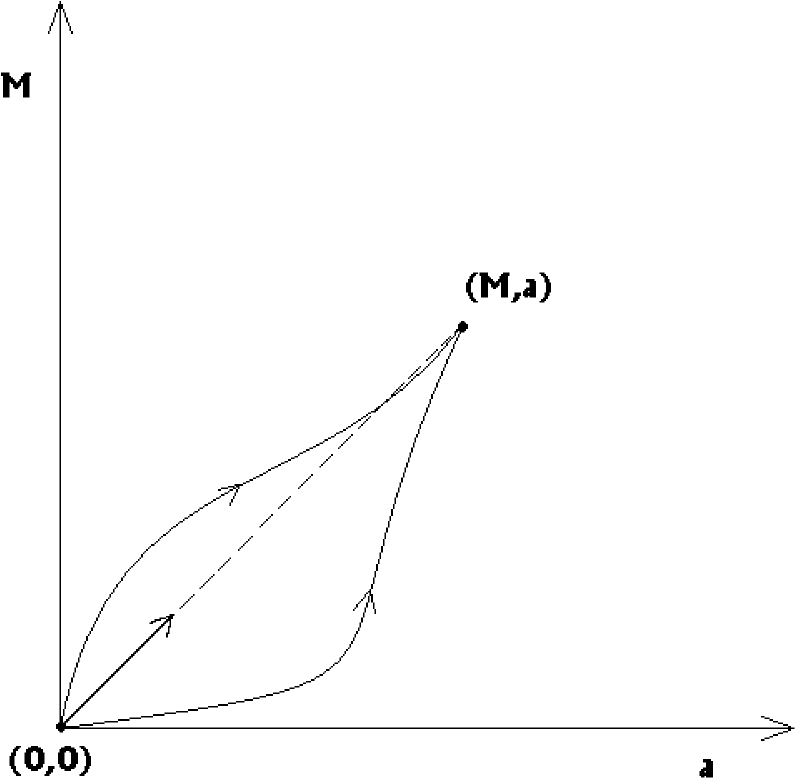
So far, in order to compute the charges the idea was to “go to infinity and stay there” [31]. What allows one to “go into the bulk” is the following modification of the $n-2$ forms $k_{\bar{\xi}}[h,\bar{g}]$: consider a path $\gamma$ in the space of solutions $g_{\mu\nu}$ to Einstein’s equations that interpolates between the background $\bar{g}_{\mu\nu}$ and a given solution $g_{\mu\nu}$ and let $\xi^{\mu}_{\gamma}$ be a Killing vector field for all the metrics along this path. Let $d_{V}g_{\mu\nu}$ denote a 1-form on the space of metrics (see e.g. [32, 33, 34] for more details). The $n-2$ form in coordinate space

$$K_{\xi;\gamma}=\int_{\gamma}k_{\xi_{\gamma}}[d_{V}g;g]$$ (3.1)

obtained by integrating $k_{\xi_{\gamma}}[d_{V}g;g]$, which is a 1-form in field space, along the path $\gamma$ can be shown to be closed wherever the interpolation is meaningful,

$$dK_{\xi;\gamma}=0,$$ (3.2)

unlike the $n-2$ forms $k_{\bar{\xi}}[h,\bar{g}]$, which are merely closed “at infinity”.

Explicitly, let $g^{(s)}_{\mu\nu}$ with $s\in[0,1]$ denote a one parameter family of solutions to Einstein’s equations interpolating between the background $\bar{g}_{\mu\nu}=g^{(0)}_{\mu\nu}$ and the given solution $g_{\mu\nu}=g^{(1)}_{\mu\nu}$, let $\xi^{s}$ be a Killing vector field for this family, $\mathcal{L}_{\xi^{(s)}}g^{(s)}_{\mu\nu}=0$, $\xi^{(0)}=\bar{\xi}$, $\xi^{(1)}=\xi$, and $h^{(s)}_{\mu\nu}=\frac{d}{ds}g^{(s)}_{\mu\nu}$ be the tangent vector to $g^{(s)}_{\mu\nu}$ in solution space. We have

$$K_{\xi;\gamma}=\int_{0}^{1}ds\,k_{\xi^{(s)}}[h^{(s)};g^{(s)}].$$ (3.3)

It follows from Stokes theorem that the charges

$$Q_{\xi;\gamma}=\oint_{S}K_{\xi;\gamma}$$ (3.4)

do not depend on the closed $n-2$ dimensional hypersurface $S$ used for their evaluation

$$\oint_{S}K_{\xi;\gamma}=\oint_{S^{\prime}}K_{\xi;\gamma}.$$ (3.5)

Figure 1: In the example of the four-dimensional Kerr black holes, the solution space is parameterized by the mass $M$ and rotation parameter $a$. One can for instance use the diagonal path $sM,sa$, $s\in[0,1]$ for the evaluation of the charges $Q_{\xi}$.

3.2 Path independence

The natural questions to ask for the charges $Q_{\xi;\gamma}$ are whether they depend on the path $\gamma$ used in their definition and what their relation with the charges $Q^{\infty}_{\xi}$ defined at infinity is.

Suppose that the dependence on $s$ of $g^{s}_{\mu\nu}(x)$ and $\xi^{s}$ is analytical and that in an expansion according to $s$ all terms which are of order $s$ or higher vanish when one approaches the boundary at infinity,

$$K_{\xi;\gamma}\longrightarrow k_{\tilde{\xi}}[h,\bar{g}],$$ (3.6)

with $h=h^{(0)}$. Because the charges $Q_{\xi;\gamma}$ can be evaluated on the surface $S^{\infty}$ at infinity, one finds, under this assumption, that they agree with the charges defined at infinity, $Q_{\xi;\gamma}=\oint_{S^{\infty}}k_{\tilde{\xi}}[h,\bar{g}]=Q^{\infty}_{\xi}$. Furthermore, the charges $Q_{\xi;\gamma}$ then do not depend on the path, but only on the initial solution $\bar{g}_{\mu\nu}(x)$ and the final solution $g_{\mu\nu}(x)$. This follows because, when evaluated at $S^{\infty}$, the charges are manifestly path independent since only the initial solution and the tangent vector pointing towards the final solution is involved. Since furthermore, the charges do not depend on the surface used for their evaluation, this remains true when they are evaluated at other surfaces $S$ in the bulk.

For the Kerr AdS black holes considered below, the angular momenta will be manifestly path independent, while we will show that the mass is integrable because (3.6) holds.

Alternatively, in order to investigate path independence of the charges $Q_{\xi;\gamma}$, one can study the integrability conditions [17, 35]

$$\oint_{S}d_{V}k_{\xi}[d_{V}g;g]=0.$$ (3.7)

In the appendix, we will show that it follows directly from the construction of the integrands $k_{\xi}[d_{V}g;g]$ that the weak integrability conditions

$$d(d_{V}k_{\xi}[d_{V}g;g])|_{\delta g,\delta\xi;g,\xi}=0$$ (3.8)

hold when $d_{V}k_{\xi}[d_{V}g;g]$ is evaluated for any $g_{\mu\nu},\delta_{1}g_{\mu\nu},\delta_{2}g_{\mu\nu}$, $\xi^{\mu}$, $\delta_{1}\xi^{\mu},\delta_{2}\xi^{\mu}$ such that

1. $g_{\mu\nu}(x)$ is a solution to Einstein’s equations,

2. $\delta g_{\mu\nu}(x)$ is a solution to the linearized Einstein’s equations,

3. $\xi^{\mu}(x)$ is a Killing vector for $g_{\mu\nu}(x)$,

4. $\delta\xi^{\mu}(x)$ satisfies the linearized Killing equation $\mathcal{L}_{\xi}\delta g_{\mu\nu}+\mathcal{L}_{\delta\xi}g_{\mu\nu}=0$.

Furthermore, we will also show that if there is no De Rham cohomology in degree $2$ in solution space and no De Rham cohomology in degree $n-2$ in $x^{\mu}$, the integrability conditions (3.8) do indeed guarantee integrability, i.e., path independence of the charges $Q_{\xi;\gamma}$.

It turns out however that, since the charges are usually integrated over closed $n-2$ dimensional surfaces, there is precisely one non vanishing De Rham cohomology class $c^{n-2}(x,dx)$ in form degree $n-2$. In the absence of De Rham cohomology in degree $2$ in solution space, this class represents the only obstruction for the weak integrability conditions (3.8) to guarantee conditions (3.7) and thus path independence of the charges: $(d_{V}k_{\xi}[d_{V}g;g])|_{\delta g,\delta\xi;g,\xi}=kc^{n-2}+d(\cdot)$, with $k$ a two form in solution space.

In the following, we will assume that there is no such obstruction ($k=0$) and denote the path independent charges simply by $Q_{\xi}$. It should be kept in mind however, that the charge related to the solution $g_{\mu\nu}$ with Killing vector $\xi$ is measured with respect to the background solution $\bar{g}_{\mu\nu}$ with Killing vector $\bar{\xi}$.

Note that any of the equivalent expressions (2.2), (2.5), (2.8), (2.9) (or (2.14), if $x^{0}$ is constant) can be used to define the charges at infinity and also the improved charges defined in (3.3). For convenience, we shall use expression (2.9), because the interpretation of the various terms will be particularly simple. Indeed, in this case, one gets

$$Q_{\xi}=-\oint_{S}K^{K}_{\xi}[g]+\oint_{S}K^{K}_{\bar{\xi}}[\bar{g}]+\oint_{S}\mathcal{C}_{\xi;\gamma},$$ (3.9)

$$\mathcal{C}_{\xi;\gamma}=\int_{0}^{1}ds\left(K^{K}_{\frac{d}{ds}\xi^{s}}[g^{(s)}]-\xi^{(s)}\cdot\Theta[h^{(s)};g^{(s)}]\right),$$ (3.10)

and the subtracted Komar integral appears explicitly. Note also that since both $Q_{\xi}$ and $-\oint_{S}K^{K}_{\xi}[g]+\oint_{S}K^{K}_{\bar{\xi}}[\bar{g}]$ are path independent, so is $\oint_{S}\mathcal{C}_{\xi;\gamma}$.

4 Geometric derivation of generalized Smarr relation

4.1 Generalized Smarr relation

We shall now show that the generalized Smarr relation follows directly by evaluating the identity (3.5), where $S=S^{\infty}$, the $n-2$ sphere at infinity and $S^{\prime}$ is chosen as an $n-2$ dimensional surface $H$ on the horizon.

More precisely, consider a black hole $g_{\mu\nu}$ with Killing horizon determined by $\xi=k+\Omega_{a}m^{a}$, where $k$ denotes the time-like Killing vector, $\Omega_{a}$ the angular velocities and $m^{a}$ the axial Killing vectors. The total energy of spacetime is defined to be $\mathcal{E}\equiv Q_{k}$, while the total angular momenta are $\mathcal{J}^{a}\equiv-Q_{m^{a}}$. In the particular case where $S^{\infty}$ is chosen tangent to $m^{a}$ and if the Killing vectors $m^{a}$ do not vary along the path $\gamma$, equation (3.9) reduces to the standard expression for the angular momenta in terms of Komar integrals:

$$\mathcal{J}^{a}=\oint_{S^{\infty}}K^{K}_{m^{a}}[g]-\oint_{S^{\infty}}K^{K}_{m^{a}}[\bar{g}].$$ (4.1)

For other surfaces or if the Killing vectors $m^{a}$ vary, the angular momenta have to be computed with the more general expression (3.9), or, if appropriate boundary conditions are fulfilled, with the expressions (2.2), (2.5), (2.8), (2.9) (or (2.14) if $x^{0}$ is constant on $S^{\infty}$).

Suppose that there exists a path $g^{(s)}_{\mu\nu}$ in solution space interpolating between the background $g^{(0)}_{\mu\nu}=\bar{g}_{\mu\nu}$ and the black hole $g^{(1)}_{\mu\nu}=g_{\mu\nu}$ with $k_{(s)}$ and $m^{a}_{(s)}$ Killing vectors along the whole path reducing to $k,m^{a}$ at the end point $g_{\mu\nu}$ of the path. It is not assumed that there is a horizon defined for all the metrics along the path. The Killing vector $\xi^{(s)}$ along the path of metrics is chosen as $\xi^{(s)}=k^{(s)}+\Omega^{(1)}_{a}m^{a}_{(s)}$, where $\Omega^{(1)}_{a}\equiv\Omega_{a}$ are the angular velocities of the horizon of the final black hole described by $g_{\mu\nu}$. Note that the Killing vector $\xi^{(s)}$ is then not the generator of the Killing horizon for the metrics $g_{\mu\nu}^{(s)}$ even when those metrics do describe black holes.

We have

$$\mathcal{E}=\oint_{S^{\infty}}K_{k;\gamma} = \oint_{S^{\infty}}K_{\xi-\Omega_{a}m^{a};\gamma}=\oint_{H}K_{\xi;\gamma}+\Omega_{a}\mathcal{J}^{a}.$$ (4.2)

The Komar integral $\oint_{H}K^{K}_{\xi}[g]$ evaluated on the horizon is well known [1] to give $\frac{\kappa}{8\pi}\mathcal{A}$ (see also e.g. [5]), where $\mathcal{A}$ is the area of the horizon. We thus get

$$\mathcal{E}-\Omega_{a}\mathcal{J}^{a}=\frac{\kappa}{8\pi}\mathcal{A}+\oint_{H}K^{K}_{\xi}[\bar{g}]+\oint_{H}\mathcal{C}_{\xi;\gamma}.$$ (4.3)

The claim is that this relation gives the generalized Smarr formula, which becomes the thermodynamical Euler relation, with the standard identifications of temperature as $\mathcal{T}=\frac{\kappa}{2\pi}$ and entropy as $\mathcal{S}=\frac{1}{4}\mathcal{A}$.

4.2 The four-dimensional Schwarzschild black hole

In order to gain some experience, let us quickly discuss the four-dimensional Schwarzschild black hole, where $\Omega_{a}=0$ and $\xi=k$. The only path interpolating between the flat background and a given solution can be parameterized by replacing $M$ by $sM$, $s\in[0,1]$, in the Schwarzschild solution in standard spherical coordinates. It is then straightforward to verify that (3.6) holds and $\mathcal{E}=M$. Furthermore, the second term on the right hand side does not contribute for the flat background $\bar{g}_{\mu\nu}=\eta_{\mu\nu}$. We then can compute $\oint_{H}\mathcal{C}_{\xi}$ in two ways:

1. Since the Komar integral is conserved by itself, $dK^{K}_{\xi}=0$, we also have $d\mathcal{C}_{\xi}=0$. We thus can move back out to infinity: $\oint_{H}\mathcal{C}_{\xi}=\oint_{S^{\infty}}\mathcal{C}_{\xi}$. There, we can either compute $\mathcal{C}_{\xi}$ directly or use the following arguments: (i) in standard spherical coordinates $\xi=\frac{\partial}{\partial t}$ is constant, so that $\mathcal{C}_{\frac{\partial}{\partial t}}$ reduces to the $\Theta$ term, (ii) because of the fall-off conditions, higher order terms in $s$ do not contribute at infinity so that $\oint_{S^{\infty}}\mathcal{C}_{\frac{\partial}{\partial t}}=-\oint_{S^{\infty}}\frac{\partial}{\partial t}\cdot\Theta[h;\bar{g}]$, (iii) the total mass at infinity is given by $-\oint_{S^{\infty}}(K^{K}_{\frac{\partial}{\partial t}}+\frac{\partial}{\partial t}\cdot\Theta[h;\bar{g}])=M$, (see e.g. [16]), (iv) since $-\oint_{S^{\infty}}K^{K}_{\frac{\partial}{\partial t}}=\mathchoice{\raisebox{0.5pt}{\footnotesize$\displaystyle\frac{1}{2}$}\kern 1.0pt}{\frac{1}{2}}{\frac{1}{2}}{\frac{1}{2}}M$ (see e.g. [1]) it follows that $\oint_{S^{\infty}}\mathcal{C}_{\frac{\partial}{\partial t}}=\frac{1}{2}M$. Injecting into (4.3), this yields $\mathchoice{\raisebox{0.5pt}{\footnotesize$\displaystyle\frac{1}{2}$}\kern 1.0pt}{\frac{1}{2}}{\frac{1}{2}}{\frac{1}{2}}M=\frac{\kappa}{8\pi}\mathcal{A}$ as it should.

2. Alternatively, one can compute $\oint_{H}\mathcal{C}_{\xi}$ directly on the horizon, or even better, following [16], on the bifurcation surface $B$, where $\xi^{s}=0$, so that now only the first term in $\mathcal{C}_{\xi}$ will contribute. Indeed, if one chooses the path $g^{s}_{\mu\nu}$ by replacing $M$ through $sM$ in the Schwarzschild solution, one has, in Kruskal coordinates, $\xi^{s}=\kappa^{s}(-U\frac{\partial}{\partial U}+V\frac{\partial}{\partial V})$ where $\kappa^{s}=\frac{1}{4sM}$. In these coordinates, the integral $\oint_{B}C_{\xi}=\oint_{B}\int^{1}_{0}ds\,K^{K}_{\frac{d\xi^{s}}{ds}}[g^{s}]$ becomes $\int_{0}^{1}ds\,\frac{4\pi(2Ms)^{2}}{16\pi}(-\partial_{V}(\frac{d\xi^{V}}{ds})+\partial_{U}(\frac{d\xi^{U}}{ds}))=\frac{1}{2}M$, as it should.

For the higher dimensional Kerr-AdS black holes discussed below, although the explicit computations are a bit more involved, the derivation of the generalized Smarr relation will also follow directly from evaluation of (4.3).

5 Application to Kerr-AdS black holes

5.1 Description of the solutions

The general Kerr Anti-de Sitter metrics in $n=2N+1+\epsilon$ dimensions, where $\epsilon\equiv n-1\text{ mod }2$ were obtained in [36, 37]. They have $N$ independent rotation parameters $a_{a}$ in $N$ orthogonal 2-planes. Gibbons et al. start from the $n$ dimensional anti-de Sitter metric in static coordinates,

$$\bar{ds}^{2}=-(1+y^{2}l^{-2})dt^{2}+\frac{dy^{2}}{1+y^{2}l^{-2}}+y^{2}\sum_{a=1}^{N}\hat{\mu}^{2}_{a}d\phi_{a}^{2}+y^{2}\sum_{i=1}^{N+\epsilon}d\hat{\mu}^{2}_{i},$$ (5.1)

with $\sum_{i=1}^{N+\epsilon}\hat{\mu}_{i}^{2}=1$. They then consider the change of variables to Boyer-Linquist spheroidal coordinates $(\tau,r,\varphi_{a},\mu_{i})$. These coordinates depend on $N$ arbitrary parameters $a_{a}$ and are defined by

$$y^{2}\hat{\mu}_{i}^{2}=\frac{(r^{2}+a_{i}^{2})}{\Xi_{i}}\mu_{i}^{2},\qquad\varphi_{a}=\phi_{a},\qquad\tau=t.$$ (5.2)

Note that for later convenience, we have renamed the variables $t,\phi^{a}$ as $\tau,\varphi^{a}$ already at this stage. The anti-de Sitter metric then becomes

$$\bar{ds}^{2} = -W(1+r^{2}l^{-2})d\tau^{2}+\frac{U}{V}\,dr^{2}+\sum_{a=1}^{N}\frac{r^{2}+a^{2}_{a}}{\Xi_{a}}\mu_{a}^{2}d{\varphi}_{a}^{2}$$

$$+\sum_{i=1}^{N+\epsilon}\frac{r^{2}+a^{2}_{i}}{\Xi_{i}}d\mu_{i}^{2}-\frac{l^{-2}}{W(1+r^{2}l^{-2})}\big{(}\sum_{i=1}^{N+\epsilon}\frac{r^{2}+a_{i}^{2}}{\Xi_{i}}\mu_{i}d\mu_{i}\big{)}^{2},$$

where

$$W \equiv \sum_{i=1}^{N+\epsilon}\frac{\mu_{i}^{2}}{\Xi_{i}},\qquad U\equiv r^{\epsilon}\sum_{i=1}^{N+\epsilon}\frac{\mu_{i}^{2}}{r^{2}+a^{2}_{i}}\prod_{a=1}^{N}(r^{2}+a_{a}^{2}),\quad\sum_{i=1}^{N+\epsilon}\mu_{i}^{2}=1,$$ (5.4)

$$V \equiv r^{\epsilon-2}(1+r^{2}l^{-2})\prod_{a=1}^{N}(r^{2}+a^{2}_{a}),\qquad\Xi_{i}\equiv 1-a_{i}^{2}l^{-2},$$ (5.5)

In the coordinates $(\tau,r,\varphi^{a},\mu^{i})$, the Kerr-AdS solutions $g_{\mu\nu}$, depending on $N+1$ parameters $M,a_{a}$, are related to the AdS metric $\bar{g}_{\mu\nu}$ as follows:

$${ds}^{2}=\bar{ds}^{2}|_{\eqref{adstilde}}+\frac{2M}{U}\big{(}W\,d\tau-\sum_{a=1}^{N}\frac{a_{a}\mu_{a}^{2}}{\Xi_{a}}\,d{\varphi}_{a}\big{)}^{2}+\frac{2MU}{V(V-2M)}\,dr^{2}.$$ (5.6)

as can be directly verified by comparing with equation (4.2) of [7]. In these coordinates, defining the metric deviations $h_{\mu\nu}$ through

$$ds^{2}=\bar{ds}^{2}|_{\eqref{adstilde}}+h_{\mu\nu}dx^{\mu}\text{d}x^{\nu}$$ (5.7)

and using $U=r^{n-3}+o(r^{n-3})$, $V=r^{n-1}l^{-2}+o(r^{n-1})$, it is straightforward to see that

$$h_{AB}\sim O(r^{-n+3}),\quad h_{rr}\sim O(r^{-n-1}),$$ (5.8)

with $A=(\tau,\varphi_{a})$, while all other components of $h_{\mu\nu}$ vanish.

The Killing vectors of the Kerr metric are given in coordinates $(t,y,\phi_{a},\hat{\mu}_{i})$ and $(\tau,r,\varphi_{a},\mu_{i})$ by

$$k\equiv\frac{\partial}{\partial t}=\frac{\partial}{\partial\tau},\qquad m^{a}\equiv\frac{\partial}{\partial\phi_{a}}=\frac{\partial}{\partial\varphi_{a}}.$$ (5.9)

5.2 Mass and angular momenta

Useful integrals

Let us define the spheroid $S^{\infty}$ in coordinates $(\tau,r,\varphi_{a},\mu_{i})$ by $r=cst\longrightarrow\infty$, $\tau=cst$. Using $\sqrt{-g}=\sqrt{-\bar{g}}$ given explicitly in equation (A.9) of [7] and expressing $\mu_{N+\epsilon}$ as a function of the remaining $\mu_{\alpha}$, $1\,{\leqslant}\,\alpha\,{\leqslant}\,N+\epsilon-1$, it is straightforward to show that

$$\mathcal{A}^{sphoid} \equiv \int_{S^{\infty}}\prod_{\alpha=1}^{N+\epsilon-1}d\mu_{\alpha}\prod_{a=1}^{N}d\varphi_{a}\ \frac{\sqrt{-\bar{g}}}{r^{n-2}}=\frac{\mathcal{A}_{n-2}}{\prod_{a=1}^{N}\Xi_{a}},$$ (5.10)

where $\mathcal{A}_{n-2}$ is the volume of the unit $n-2$ sphere, given explicitly for instance in (4.9) of [7].

Similarly,

$$\mathcal{I} \equiv \int_{S^{\infty}}\prod_{\alpha=1}^{N+\epsilon-1}d\mu_{\alpha}\prod_{a=1}^{N}d\varphi_{a}\ \frac{\sqrt{-\bar{g}}}{r^{n-2}}\,W=\frac{2}{n-1}\big{(}\sum_{a=1}^{N}\frac{1}{\Xi_{a}}+\frac{\epsilon}{2}\,\big{)}\mathcal{A}^{sphoid}.$$ (5.11)

This identity has been verified using Mathematica up to $n=8$. We suppose it holds for higher $n$.

Choosing a path

The path $\gamma$ joining the AdS background to the Kerr-AdS metric is chosen as follows: for $s\in[0,1]$, $g^{s}_{\mu\nu}$ is obtained by replacing $M$ by $sM$ in (5.6).

Angular momenta

Because $m^{a}=\frac{\partial}{\partial\varphi_{a}}$ is tangent to $S^{\infty}$ and does not vary along the path $\gamma$, one can use (4.1) instead of (3.9) to compute the angular momenta $\mathcal{J}^{a}$. Explicitly, one gets

$$\mathcal{J}^{a} = \int_{S^{\infty}}\prod_{\alpha=1}^{N+\epsilon-1}d\mu_{\alpha}\prod_{a=1}^{N}d\varphi_{a}\ \frac{\sqrt{-\bar{g}}}{16\pi}\left(g^{\tau\alpha}g^{rr}g_{\alpha\varphi^{a},r}-\bar{g}^{\tau\alpha}\bar{g}^{rr}\bar{g}_{\alpha\varphi^{a},r}\right)$$ (5.12)

$$= \frac{Ma_{a}}{8\pi}(n-1)\int_{S^{\infty}}\prod_{\alpha=1}^{N+\epsilon-1}d\mu_{\alpha}\prod_{a=1}^{N}d\varphi_{a}\ \frac{\sqrt{-g}}{r^{n-2}}\frac{\mu_{a}^{2}}{\Xi_{a}}=\frac{Ma_{a}}{4\pi\Xi_{a}}\,\mathcal{A}^{sphoid}.$$

Here, the Komar integral evaluated for the background does not contribute because $\bar{g}_{\tau\varphi_{a}}=\bar{g}^{\tau\varphi_{a}}=0$. The result agrees with the one given in [7].

Mass

In order to compute the mass, we evaluate (3.9) with $\xi=k=\frac{\partial}{\partial\tau}$ on $S^{\infty}$. We have

$$\int_{S^{\infty}}(-K^{K}_{k}[g]+K^{K}_{k}[\bar{g}]) =$$

$$\int_{S^{\infty}}\prod_{\alpha=1}^{N+\epsilon-1}d\mu_{\alpha}\prod_{a=1}^{N}d\varphi_{a}\ \frac{\sqrt{-\bar{g}}}{16\pi}\left(g^{\tau\alpha}g^{rr}g_{\alpha\tau,r}-{\bar{g}}^{\tau\alpha}{\bar{g}}^{rr}{\bar{g}}_{\alpha\tau,r}\right).$$ (5.13)

Let decompose the metric as $g_{\mu\nu}=\bar{g}_{\mu\nu}+h_{\mu\nu}$. The asymptotic behavior (5.8) of $h_{\mu\nu}$ implies that $h^{\mu}_{\,\,\nu}=\bar{g}^{\mu\alpha}h_{\alpha\nu}=O(r^{-n+1})$. Hence, in the expansion of the inverse metric $g^{\mu\nu}$

$$g^{\mu\nu}=\bar{g}^{\mu\alpha}(\delta^{\,\,\nu}_{\alpha}-h^{\,\,\nu}_{\alpha}+h^{\,\,\beta}_{\alpha}h^{\,\,\nu}_{\beta}-h^{\,\,\gamma}_{\alpha}h^{\,\,\beta}_{\gamma}h^{\,\,\nu}_{\beta}+\cdots).$$ (5.14)

only the first two terms will contribute to integral (5.13), since the following terms fall off faster and keeping only the first two terms will give finite contributions, as we will show. Injecting this expansion into (5.13), one gets terms that are at most quadratic in $h_{\mu\nu}$. The terms of order $0$ will cancel, while the terms quadratic in $h_{\mu\nu}$ can directly be shown not to contribute. Hence, only terms linear in $h_{\mu\nu}$ will contribute to (5.13) with the result

$$\int_{S^{\infty}}(-K^{K}_{k}[g]+K^{K}_{k}[\bar{g}]) = \frac{M}{8\pi}\int_{S^{\infty}}\prod_{\alpha=1}^{N+\epsilon-1}d\mu_{\alpha}\prod_{a=1}^{N}d\varphi_{a}\ \frac{\sqrt{-\bar{g}}}{r^{n-2}}\Big{[}(n-1)W-2\Big{]}$$ (5.15)

$$= \frac{M\mathcal{A}_{n-2}}{4\pi(\prod_{a}\Xi_{a})}\left(\sum_{b=1}^{N}\frac{1}{\Xi_{b}}+\frac{\epsilon}{2}-1\right).$$

The integral $\oint_{S^{\infty}}\mathcal{C}_{k;\gamma}$ defined in (3.10) reduces to the integral of the $\xi\cdot\Theta$ part which reads

$$\oint_{S^{\infty}}\mathcal{C}_{k;\gamma}=\int_{0}^{1}ds\,\int_{S^{\infty}}\prod_{\alpha=1}^{N+\epsilon-1}d\mu_{\alpha}\prod_{a=1}^{N}d\varphi_{a}\ \frac{\sqrt{-\bar{g}}}{16\pi}(D^{(s)}_{\sigma}h_{(s)}^{r\sigma}-\partial^{r}h_{(s)}),$$ (5.16)

where the integrand (but not the integral) depends explicitly on the path through $g^{(s)}_{\mu\nu}$, $h^{(s)}_{\mu\nu}=\frac{dg^{(s)}_{\mu\nu}}{ds}$ (and indices are lowered and raised with $g^{(s)}_{\mu\nu}$ and its inverse). Note that the equality $\sqrt{-g^{(s)}}=\sqrt{-\bar{g}}$ implies $h^{(s)}=0$. From the definition of the metric (5.6), one can see that

$$h^{(s)}_{\mu\nu}=h_{\mu\nu}+o(h_{\mu\nu}),\quad g^{(s)}_{\mu\nu}=\bar{g}_{\mu\nu}+sh_{\mu\nu}+o(h_{\mu\nu}),$$ (5.17)

where $\bar{g}_{\mu\nu}$ is the AdS metric and $h_{\mu\nu}$ is defined in (5.7). Now, as the leading terms in expression (5.17) give finite contributions to the integral (5.16), as we will show below, the sub-leading terms $o(h_{\mu\nu})$ will not contribute. Expanding $g^{\mu\nu}_{(s)}$ as in (5.14), we get

$$g_{(s)}^{\mu\nu}\sim\bar{g}^{\mu\alpha}(\delta^{\,\,\nu}_{\alpha}-sh^{\,\,\nu}_{\alpha}+s^{2}h^{\,\,\beta}_{\alpha}h^{\,\,\nu}_{\beta}-\cdots),$$ (5.18)

where the indices are raised with $\bar{g}^{\mu\nu}$ and where $\sim$ indicates that the sub-leading terms in equation (5.17) have been dropped. Again, we will show below that the first two terms of (5.18) give finite contributions to the integral (5.16). As the following terms in (5.18) fall off faster, we can safely ignore them in the computation. If we now expand the expressions $g_{\mu\nu}^{(s)}$, $g_{(s)}^{\mu\nu}$ and $h_{\mu\nu}^{(s)}$ in the integrand $\sqrt{-\bar{g}}D^{(s)}_{\sigma}h_{(s)}^{r\sigma}$ in terms of $\bar{g}_{\mu\nu}$ and of $h_{\mu\nu}$, we obtain after some work that

$$\sqrt{-\bar{g}}D^{(s)}_{\sigma}h_{(s)}^{r\sigma}=\sqrt{-\bar{g}}{\bar{D}}_{\sigma}h^{r\sigma}+O(r^{-n+1})$$ (5.19)

where all the dependence in $s$ appear only in the vanishing term $O(r^{-n+1})$. Because $h=0$, we have thus shown that $\oint_{S^{\infty}}\mathcal{C}_{k;\gamma}$ reduces to the integral over $S^{\infty}$ of the third term of (2.9), with $\xi=k$. Hence, we have shown that at $S^{\infty}$, the mass (and, as we have seen before, the angular momenta as well) can be computed using any one of the equivalent expressions (2.2), (2.5), (2.8), (2.9) and (2.14) (since $\tau$ is constant on $S^{\infty}$) of the linearized theory.

Explicitly, one shows after some computations that $D_{\sigma}h^{r\sigma}$ reduces to $r^{-1}h^{rr}+o(r^{-n+2})$. Therefore, $\oint_{S^{\infty}}\mathcal{C}_{k;\gamma}$ becomes

$$\oint_{S^{\infty}}\mathcal{C}_{k;\gamma} = \frac{M}{8\pi}\mathcal{A}^{sphoid}=\frac{M}{8\pi}\frac{\mathcal{A}_{n-2}}{(\prod_{a}\Xi_{a})}.$$ (5.20)

Finally, the energy (3.9) is obtained by summing the two contributions $\oint(-K^{K}_{k}[g]+K^{K}_{k}[\bar{g}])$ and $\oint\mathcal{C}_{k;\gamma}$, which gives explicitly

$$\mathcal{E}=\frac{M\mathcal{A}_{n-2}}{4\pi(\prod_{a}\Xi_{a})}\left(\sum_{b=1}^{N}\frac{1}{\Xi_{b}}-\frac{(1-\epsilon)}{2}\right),$$ (5.21)

in agreement with [7, 8].

5.3 Generalized Smarr relation

We now evaluate the remaining terms in the Smarr relation (4.3).

The integral $\oint_{H}K^{K}_{\xi}[\bar{g}]$ evaluated on the surface $r=r_{+}$, where the horizon radius $r_{+}$ is the largest root of $V(r)-2m=0$, is given by

$$\oint_{H}K^{K}_{\xi}[\bar{g}]=-\frac{\mathcal{A}_{n-2}}{8\pi l^{2}(\prod_{a}\Xi_{a})}r_{+}^{\epsilon}\prod_{a=1}^{N}(r_{+}^{2}+a^{2}_{a}).$$ (5.22)

Note that this integral vanishes in Minkowski space $(l\rightarrow\infty)$.

In Kerr-AdS spacetimes, the Komar integrand $K^{K}_{\xi}$ of a Killing vector $\xi$ is not closed. Indeed, using the equations of motion $R_{\mu\nu}=-(n-1)l^{-2}g_{\mu\nu}$, we have

$$dK^{K}_{\xi}[g] = \frac{1}{16\pi}(d^{n-1}x)_{\nu}\sqrt{-g}\big{(}D_{\mu}D^{\mu}\xi^{\nu}-D_{\mu}D^{\nu}\xi^{\mu}\big{)}$$ (5.23)

$$= -\frac{n-1}{8\pi l^{2}}(d^{n-1}x)_{\nu}\sqrt{-g}\xi^{\nu}.$$ (5.24)

Because $\sqrt{-g}=\sqrt{-\bar{g}}$, we have $d(-K^{K}_{\xi}[g]+K^{K}_{\xi}[\bar{g}])=0$. It then follows from the definition of $\mathcal{C}_{\xi;\gamma}$ (see equation (3.9)) and from the identity $dK_{\xi;\gamma}=0$ that $d\,\mathcal{C}_{\xi;\gamma}=0$. We thus can move the integral on the horizon back out to infinity,

$$\oint_{H}\mathcal{C}_{\xi;\gamma}=\oint_{S^{\infty}}\mathcal{C}_{k;\gamma}+\Omega_{a}\oint_{S^{\infty}}\mathcal{C}_{m^{a};\gamma}.$$ (5.25)

The first term on the right hand side has already been computed in (5.20), while the second term vanishes because $m^{a}=\frac{\partial}{\partial\varphi^{a}}$ does not vary along the path and is tangent to $S^{\infty}$.

We can now write the Smarr formula (4.3) as

$$\mathcal{E}-\Omega_{a}\mathcal{J}^{a} = \frac{\kappa\mathcal{A}^{sphoid}}{8\pi}+\frac{\mathcal{A}^{sphoid}}{8\pi}\big{(}M-\frac{r_{+}^{\epsilon}}{l^{2}}\prod_{b=1}^{N}(r_{+}^{2}+a^{2}_{b})\big{)},$$ (5.26)

in complete agreement with the results obtained by Euclidean methods in [7].

In the limit $l\rightarrow\infty$, we recover the Smarr formula for Kerr black holes in flat backgrounds since then $\mathcal{A}^{sphoid}=\mathcal{A}_{n-2}$, $\oint_{H}K^{K}_{\xi}[\bar{g}]=0$. Combining (5.20) with (5.21) then gives $\oint\mathcal{C}_{\xi}=(n-2)^{-1}\mathcal{E}$. Injected into (4.3), we finally have

$$\frac{n-3}{n-2}\mathcal{E}-\Omega_{a}\mathcal{J}^{a} = \frac{\kappa\mathcal{A}_{n-2}}{8\pi}.$$ (5.27)

Appendix A Integrability of charges for trivial de Rham cohomology

In this appendix, we follow the notation of [22], appendix A. More details can be found in [32]. Note however that in the considerations below we are considering jet spaces where the fibers include not only the fields $\phi^{i}$ and their derivatives, but also the gauge parameters $f^{\alpha}$. We will use the notation $\phi^{\Delta}\equiv(\phi^{i},f^{\alpha})$.

In particular, $S=\int d^{n}x\,L$ is the action of a local gauge field theory (e.g., the Einstein-Hilbert action), $\phi^{i}$ are the fields (e.g., $g_{\mu\nu}$), $f^{\alpha}$ the gauge parameters (e.g., $\xi^{\mu}$) and $R^{i}_{\alpha}(f^{\alpha})$ denote a generating set of gauge transformations (e.g., $\mathcal{L}_{\xi}g_{\mu\nu}$). The weakly vanishing Noether current $S_{f}$ is defined through

$${\frac{\delta L}{\delta\phi^{i}}}R^{i}_{\alpha}(f^{\alpha})d^{n}x=d_{H}S_{f},\ S_{f}\equiv S^{i}_{\alpha}({\frac{\delta L}{\delta\phi^{i}}},f^{\alpha}).$$ (A.1)

If $\omega^{p,s}$ is a $p$ form in $dx^{\mu}$ and an $s$ form in $d_{V}\phi^{a}_{(\lambda)}$, the horizontal homotopy operator (see eq (4.13) of [32]) is defined by

$$h^{p,s}_{H}\omega^{p,s}=\frac{1}{s}\frac{|\lambda|+1}{n-p+|\lambda|+1}\partial_{(\lambda)}[d_{V}\phi^{\Delta}\frac{\delta}{\delta d_{V}\phi^{\Delta}_{(\lambda)\rho}}\frac{\partial\omega^{p,s}}{\partial dx^{\rho}}],$$ (A.2)

where a sum over the multi-index $(\lambda)$ is understood. If

$$k_{f}[d_{V}\phi;\phi]=-h^{n-1,1}_{H}d_{V}S_{f},$$ (A.3)

it follows from the homotopy formula $\omega^{p,s}=d_{H}h^{p,s}_{H}\omega^{p,s}+h^{p+1,s}_{H}d_{H}\omega^{p,s}$, valid for $s\,{\geqslant}\,1$, that

$$d_{H}k_{f}[d_{V}\phi;\phi]=-d_{V}S_{f}-h^{n,1}_{H}d_{V}\big{(}R^{i}_{\alpha}(f^{\alpha})\frac{\delta L}{\delta\phi^{i}}\big{)}d^{n}x.$$ (A.4)

This implies that sufficient conditions for the right hand side to vanish are that $\phi^{i}$ satisfies the field equations, $\frac{\delta L}{\delta\phi^{i}}|_{\phi}=0$, $\delta\phi^{i}$ satisfies the linearized field equations around $\phi^{i}$, $(d_{V}\frac{\delta L}{\delta\phi^{i}})|_{\delta\phi,\phi}=0$, and $f^{\alpha}$ is a reducibility parameter for $\phi^{i}$, $R^{i}_{\alpha}[\phi](f^{\alpha})=0$ (which, in the case of relativity, translates into the requirement that $\xi^{\mu}$ is a Killing vector).

Note that $k_{f}[d_{V}\phi;\phi]$ defined in equation (A.3) differs from the $k_{f}[d_{V}\phi;\phi]$ defined by the homotopy formula involving the $\phi^{i}$ alone (which is the one explicitly used in subsection 2.1). The additional piece will however be linear and homogeneous in $\frac{\delta L}{\delta\phi^{i}}$ and its derivatives, hence it vanishes when evaluated for solutions of the field equations and can be safely dropped for the computation of the charges. Furthermore, it will also not affect the considerations below.

Applying $d_{V}$ to this equation gives

$$d_{H}d_{V}k_{f}=d_{V}h^{n,1}_{H}d_{V}\big{(}R^{i}_{\alpha}(f^{\alpha})\frac{\delta L}{\delta\phi^{i}}\big{)}d^{n}x.$$ (A.5)

It follows that sufficient conditions for the right hand side to vanish are now that $\frac{\delta L}{\delta\phi^{i}}$, $d_{V}\frac{\delta L}{\delta\phi^{i}}$, $R^{i}_{\alpha}(f^{\alpha})$ and $d_{V}[R^{i}_{\alpha}(f^{\alpha})]$ should vanish when evaluated for $\phi^{i},f^{\alpha},\delta\phi^{i},\delta f^{\alpha}$. This proves the first claim in subsection 3.2.

For the second claim, we first note that the vertical homotopy is given by

$$h_{V}\omega^{p,s}=\int^{1}_{0}\frac{dt}{t}\big{(}\phi^{\Delta}_{(\mu)}\frac{\partial\omega^{p,s}}{\partial d_{V}\phi^{\Delta}_{(\mu)}}\big{)}[x,dx,t\phi,td_{V}\phi],$$ (A.6)

with

$$\omega^{p,s}-\omega^{p,s}[x,dx,\phi=0,d_{V}\phi=0]=d_{V}h_{V}\omega^{p,s}+h_{V}d_{V}\omega^{p,s},$$ (A.7)

and (see e.g. (4.11) of [32])

$$d_{H}h_{V}\omega^{p,s}=-h_{V}d_{H}\omega^{p,s}.$$ (A.8)

Assume now that $k_{f}[d_{V}\phi;\phi]$ is evaluated for a family of solutions $\phi^{i}_{a}$ and associated reducibility parameters $f^{\alpha}_{a}$ depending on continuous parameters $a^{A}$. In this case, the solution space can be identified with the parameter space. The differential $d_{V}$ then reduces to the exterior derivative in parameter space, $d_{a}=da^{A}\frac{\partial}{\partial a^{A}}$ and the vertical homotopy $h_{V}$ reduces to the standard de Rham homotopy operator $h_{a}$ in parameter space. In particular, the conditions discussed below equation (A.5) then hold. It follows from (A.5) that $d_{H}d_{a}k_{f_{a}}[d_{a}\phi_{a};\phi_{a}]=0$, where $d_{H}=dx^{\mu}\frac{d}{dx^{\mu}}$ reduces to the total derivative with respect to $x^{\mu}$. Because $d_{a}k_{f_{a}}[d_{a}\phi_{a};\phi_{a}]$ is a closed $n-2$ form in $dx^{\mu}$ depending on parameters $a^{A},da^{A}$, it follows, because of the assumption that there is no cohomology in degree $n-2$ in $x^{\mu}$ space, that

$$d_{a}k_{f_{a}}[d_{a}\phi_{a};\phi_{a}]=d_{H}l(a,da,x,dx),$$ (A.9)

where $l(a,da,x,dx)$ is some $n-3$ form in $dx^{\mu}$ depending on the parameters $a^{A},da^{A}$. (Note that $l(a,da,x,dx)$ is not necessarily built out of the fields and a finite number of their derivatives). Integrating over a closed $n-2$ dimensional surface $S$, we get $d_{a}\oint_{S}k_{f_{a}}[d_{a}\phi_{a};\phi_{a}]=0$. If there is no de Rham cohomology in degree $2$ in parameter space, this implies $\oint_{S}k_{f_{a}}[d_{a}\phi_{a};\phi_{a}]=d_{a}Q(a)$ for some function $Q(a)$. More precisely, in the case where the parameter space is $\mathbb{R}^{n}$, one can apply the homotopy operator $h_{a}$ and (A.8) implies that $k_{f_{a}}[d_{a}\phi_{a};\phi_{a}]=-d_{H}h_{a}l(a,da,x,dx)+d_{a}h_{a}k_{f_{a}}[d_{a}\phi_{a};\phi_{a}]$. We thus find that $Q(a)=\oint_{S}h_{a}k_{f_{a}}[d_{a}\phi_{a};\phi_{a}]$. (Again $h_{a}k_{f_{a}}[d_{a}\phi_{a};\phi_{a}]$ is not necessarily built out of the fields and a finite number of their derivatives.)

References

- [1] J. M. Bardeen, B. Carter, and S. W. Hawking, “The four laws of black hole mechanics,” Commun. Math. Phys. 31 (1973) 161–170.
- [2] B. Carter, Black holes, ch. Black hole equilibrium states, pp. 58–214. 1972 Les Houches Lectures. Gordon and Breach, New York, C. and B. DeWitt ed., 1973.
- [3] R. Arnowitt, S. Deser, and C. Misner, Gravitation, an Introduction to Current Research, ch. 7. The Dynamics of General Relativity, pp. 227–265. Wiley, New York, 1962.
- [4] R. Arnowitt, S. Deser, and C. W. Misner, “Coordinate invariance and energy expressions in general relativity,” Phys. Rev. 122 (1961) 997–1006.
- [5] P. K. Townsend, “Black holes,” gr-qc/9707012.
- [6] R. C. Myers and M. J. Perry, “Black holes in higher dimensional space-times,” Ann. Phys. 172 (1986) 304.
- [7] G. W. Gibbons, M. J. Perry, and C. N. Pope, “The First Law of Thermodynamics for Kerr-Anti-de Sitter Black Holes,” hep-th/0408217.
- [8] N. Deruelle and J. Katz, “On the mass of a Kerr-anti-de Sitter spacetime in d dimensions,” gr-qc/0410135.
- [9] J. Katz, J. Bicak, and D. Lynden-Bell, “Relativistic conservation laws and integral constraints for large cosmological perturbations,” Phys. Rev. D55 (1997) 5957–5969.
- [10] A. Ashtekar and A. Magnon, “Asymptotically anti-de Sitter space-times,” Class. Quant. Grav. 1 (1984) L39.
- [11] A. Ashtekar and S. Das, “Asymptotically anti-de Sitter space-times: Conserved quantities,” Class. Quant. Grav. 17 (2000) L17–L30, hep-th/9911230.
- [12] L. F. Abbott and S. Deser, “Stability of gravity with a cosmological constant,” Nucl. Phys. B195 (1982) 76.
- [13] T. Regge and C. Teitelboim, “Role of surface integrals in the Hamiltonian formulation of general relativity,” Ann. Phys. 88 (1974) 286.
- [14] M. Henneaux and C. Teitelboim, “Asymptotically anti-de Sitter spaces,” Commun. Math. Phys. 98 (1985) 391.
- [15] M. Henneaux, “Asymptotically anti-de Sitter universes in d = 3, 4 and higher dimensions,” in Proceedings of the Fourth Marcel Grossmann Meeting on General Relativity, Rome 1985, R. Ruffini, ed., pp. 959–966. Elsevier Science Publishers B.V., 1986.
- [16] V. Iyer and R. M. Wald, “Some properties of Noether charge and a proposal for dynamical black hole entropy,” Phys. Rev. D50 (1994) 846–864, gr-qc/9403028.
- [17] R. M. Wald and A. Zoupas, “A general definition of conserved quantities in general relativity and other theories of gravity,” Phys. Rev. D61 (2000) 084027, gr-qc/9911095.
- [18] B. Julia and S. Silva, “Currents and superpotentials in classical gauge invariant theories. I: Local results with applications to perfect fluids and general relativity,” Class. Quant. Grav. 15 (1998) 2173, gr-qc/9804029.
- [19] S. Silva, “On superpotentials and charge algebras of gauge theories,” Nucl. Phys. B558 (1999) 391–415, hep-th/9809109.
- [20] B. Julia and S. Silva, “Currents and superpotentials in classical gauge theories. II: Global aspects and the example of affine gravity,” Class. Quant. Grav. 17 (2000) 4733–4744, gr-qc/0005127.
- [21] I. M. Anderson and C. G. Torre, “Asymptotic conservation laws in field theory,” Phys. Rev. Lett. 77 (1996) 4109–4113, hep-th/9608008.
- [22] G. Barnich and F. Brandt, “Covariant theory of asymptotic symmetries, conservation laws and central charges,” Nucl. Phys. B633 (2002) 3–82, hep-th/0111246.
- [23] J. D. Brown and J. James W. York, “Quasilocal energy and conserved charges derived from the gravitational action,” Phys. Rev. D47 (1993) 1407–1419.
- [24] M. M. Caldarelli, G. Cognola, and D. Klemm, “Thermodynamics of Kerr-Newman-AdS black holes and conformal field theories,” Class. Quant. Grav. 17 (2000) 399–420, hep-th/9908022.
- [25] G. Barnich, “Boundary charges in gauge theories: Using Stokes theorem in the bulk,” Class. Quant. Grav. 20 (2003) 3685–3698, hep-th/0301039.
- [26] G. Barnich, F. Brandt, and M. Henneaux, “Local BRST cohomology in the antifield formalism. I. General theorems,” Commun. Math. Phys. 174 (1995) 57–92, hep-th/9405109.
- [27] G. Barnich, F. Brandt, and M. Henneaux, “Local BRST cohomology in gauge theories,” Phys. Rept. 338 (2000) 439–569, hep-th/0002245.
- [28] G. Barnich, S. Leclercq, and P. Spindel, “Classification of surface charges for a spin 2 field on a curved background solution,” gr-qc/0404006.
- [29] J. D. Brown and M. Henneaux, “Central charges in the canonical realization of asymptotic symmetries: An example from three-dimensional gravity,” Commun. Math. Phys. 104 (1986) 207.
- [30] M. Henneaux and C. Teitelboim, Quantization of Gauge Systems. Princeton University Press, 1992.
- [31] B. L. Julia, “Holography of charges in gauge theories,” Nucl. Phys. Proc. Suppl. 102 (2001) 156–160, hep-th/0104231.
- [32] I. Anderson, “The variational bicomplex,” tech. rep., Formal Geometry and Mathematical Physics, Department of Mathematics, Utah State University, 1989.
- [33] I. Anderson, “Introduction to the variational bicomplex,” in Mathematical Aspects of Classical Field Theory, M. Gotay, J. Marsden, and V. Moncrief, eds., vol. 132 of Contemporary Mathematics, pp. 51–73. Amer. Math. Soc., 1992.
- [34] P. Olver, Applications of Lie Groups to Differential Equations. Spinger Verlag, New York, 2nd ed., 1993. 1st ed., 1986.
- [35] B. Julia and S. Silva, “On covariant phase space methods,” hep-th/0205072.
- [36] G. W. Gibbons, H. Lu, D. N. Page, and C. N. Pope, “The general Kerr-de Sitter metrics in all dimensions,” hep-th/0404008.
- [37] G. W. Gibbons, H. Lu, D. N. Page, and C. N. Pope, “Rotating black holes in higher dimensions with a cosmological constant,” Phys. Rev. Lett. 93 (2004) 171102, hep-th/0409155.