News from Critical Collapse: Bondi Mass, Tails and Quasinormal Modes

Abstract

We discuss critical gravitational collapse on the threshold of apparent horizon formation as a model both for the discussion of global aspects of critical collapse and for numerical studies in a compactified context. For our matter model we choose a self-gravitating massless scalar field in spherical symmetry, which has been studied extensively in the critical collapse literature. Our evolution system is based on Bondi coordinates, the mass function is used as an evolution variable to ensure regularity at null infinity. We compute radiation quantities like the Bondi mass and news function and find that they reflect the discretely self-similar (DSS) behavior. Surprisingly, the period of radiation at null infinity is related to the formal result for the leading quasi-normal mode of a black hole with rapidly decreasing mass. Furthermore, our investigations shed some light on global versus local issues in critical collapse, and the validity and usefulness of the concept of null infinity when predicting detector signals.

I Introduction

In this paper we present a numerical study of scalar field critical collapse on the threshold of singularity formation. We consider Einstein’s equations with a minimally coupled massless scalar field $\phi$:

$$G_{ab} = 8\pi T_{ab}=\nabla_{a}\phi\nabla_{b}\phi-\frac{1}{2}g_{ab}\nabla_{c}\phi\nabla^{c}\phi,$$ (1)

$$\Box_{g}\phi = 0,$$ (2)

We restrict ourselves to the case of spherical symmetry, which has been studied extensively with numerical and analytical techniques since the discovery of critical collapse by Choptuik Choptuik (1992, 1993). We extend previous investigations by focussing on global aspects of this problem, and use a compactified evolution scheme which includes null infinity on our numerical grid. The motivation is twofold: First, we want to simplify the discussion and improve the understanding of local versus global issues in critical collapse. In particular, we try to explain questions like: What is the role of asymptotic flatness for critical collapse (e.g. the critical solution, the “Choptuon” is self-similar, and thus not asymptotically flat)? How would hypothetical detectors of radiation observe the dynamics close to criticality? How can we understand the way null infinity approximates observers at large distances in this simple but nontrivial setup? The second motivation is to test numerical algorithms which are based on compactification methods in a situation that is very demanding on accuracy. We will argue that at least in the model considered here, global methods do not cause a significant penalty in accuracy, but simplify the interpretation of certain results.

Critical phenomena in gravitational collapse have been originally discovered in the pioneering numerical investigations of Choptuik Choptuik (1992, 1993). He studied a massless scalar field coupled to gravity with sophisticated numerical techniques that allowed him to analyze the transition in the space of initial data between dispersion to infinity and the formation of a black hole. It turned out, that black holes of arbitrarily small mass can be created, and that the critical solutions approach a discretely self-similar solution, called the “Choptuon”. Both the Choptuon and the scaling law for the black hole mass are universal for arbitrary families of initial data. Hamadé and Stewart Hamade and J.M.Stewart (1996) have found numerical evidence, that the critical solution contains a naked singularity which can be seen at future null infinity. Similar critical solutions – exhibiting (continuous or discrete) self-similarity – have also been found for several other types of matter fields, and have been constructed directly in several cases Gundlach (1995, 1997a, 1997b); Lechner et al. (2002); Lechner (2001). The problem has also been studied extensively from an analytic point of view by Christodoulou Christodoulou (1986, 1987, 1991, 1994), in particular he could show that the space of regular initial data that lead to naked singularities has measure zero Christodoulou (1999).

In the current work, we refer to critical collapse phenomena as “critical collapse at the threshold of apparent horizon formation” to avoid possible misunderstandings, since critical collapse is essentially a quasilocal phenomenon and the standard definition of black holes is based on global concepts (see textbooks like e.g. Wald (1984)). Also, this term emphasizes the relation of these phenomena to other areas in nonlinear partial differential equations (PDEs), where related phenomena occur, but the concept of black holes is absent.

Critical behavior of the kind originally found by Choptuik is usually referred to as type II, because of its formal correspondence with type II phase transitions of statistical physics. A different type of critical solutions at the threshold of black hole formation, corresponding to type I phase transitions, is provided by unstable static configurations – like those found by Bartnik and McKinnon Bartnik and McKinnon (1988).

Linear perturbation calculations of such critical solutions revealed exactly one unstable mode, which confirmed their interpretation as intermediate attractors in the language of dynamical systems. Critical phenomena in general relativity are reviewed in Gundlach (1998); Bizoń (1996), including discussions in terms of phase transitions and renormalization group techniques familiar from statistical physics.

A massless scalar field in spherical symmetry exhibits type II critical collapse (there are no regular stationary or time-periodic solutions). Type II critical solutions have been found to exhibit continuous or discrete self-similarity in the past lightcone of the singularity. In our case, the critical solution is known to be discretely self-similar (DSS), and has been constructed directly as an eigenvalue problem Gundlach (1995).

A spacetime is said to be DSS Gundlach (1999) if it admits a discrete diffeomorphism $\Phi_{\Delta}$ which leaves the metric invariant up to a constant scale factor:

$$\left(\Phi^{*}_{\Delta}\right)^{n}g=e^{2n\Delta}g,$$ (3)

where $\Delta$ is a dimensionless real constant and $n\in\mathbb{N}$.

We choose scalar field critical collapse in spherical symmetry for several reasons: the model is very well studied and we can compare with a large amount of previous numerical and analytical results. Furthermore, the model is also very demanding: The value of the echoing period in the DSS critical solution is $\Delta\simeq 3.44$, which is quite larger compared to many other models. Note that larger values of $\Delta$ make it more difficult to resolve a large number of echos.

Our numerical method is based on a characteristic initial value problem, i.e. we foliate spacetime by null cones. This allows for a very efficient evolution system and simplifies the study of the causal structure of the solutions. In spherical symmetry, caustics are restricted to the center of symmetry, so we do not have to deal with the dynamical appearance of caustics, which causes potential problems for characteristic initial value problems in higher dimensions. Our numerical approach mixes techniques from previous work of Garfinkle Garfinkle (1995) and the Pittsburgh group Gómez and Winicour (1992); Winicour (1998), in particular we follow Garfinkle in moving along ingoing null geodesics to utilize gravitational focusing for increasing resolution in the region of large curvature. Furthermore, compactification methods are well studied and relatively straightforward to implement in characteristic codes.

An important aspect of our compactified characteristic evolution scheme is that at late times our null slices asymptotically approach the event horizon, see Fig. 1. Essentially this is because our coordinates can not penetrate a dynamical horizon Ashtekar and Krishnan (2002, 2003, 2004); Hayward (1994) (they become singular at a marginally trapped surface, e.g. at an apparent horizon), which is spacelike if any matter or radiation falls through it and null otherwise Hawking and Ellis (1973); Ashtekar and Krishnan (2004). Note that the dynamical horizon is contained inside of the event horizon, and the outermost dynamical horizon approaches (or coincides with) the event horizon at late times, assuming cosmic censorship holds. This fact makes our approach in some sense complementary to previous critical collapse studies, which were not adapted to the asymptotic regime. In this paper we focus on those aspects of critical collapse which are associated with global structure, and in particular the phenomenology seen by asymptotic observers. We will only make brief remarks about other well-studied aspects such as mass scaling and universality.

The paper is organized as follows: in Sec. II we give a brief introduction to scalar field critical collapse in spherical symmetry, and discuss our geometric setup, which is based on Bondi-type coordinates and a compactification scheme which introduces the Misner-Sharp mass function as an independent evolution variable, which renders our evolution system regular at null infinity. Our numerical algorithms are presented in Sec. III. In Sec. IV we give a detailed discussion of our numerical results, which include the study of power law tails, and compare the radiation signal at null infinity with a heuristic estimate based on self-similar scaling and quasi-normal mode frequencies. Our results and conclusions are summarized in Sec. V.

\psfrag{r=0}[m]{$\scriptstyle r=0$}\psfrag{i+}[m]{$\scriptstyle i^{+}$}\psfrag{i-}[m]{$\scriptstyle i^{-}$}\psfrag{i0}[m]{$\scriptstyle i^{0}$}\psfrag{scri+}[m]{$\scriptstyle{\mathscr{I}}^{+}$}\psfrag{scri-}[m]{$\scriptstyle{\mathscr{I}}^{-}$}\psfrag{H+}[m]{$\scriptstyle{\mathscr{H}}^{+}$}\includegraphics[width=130.08731pt]{spacetime_grid.eps}

Figure 1: A Penrose diagram of a typical collapse spacetime. Shown is our numerical null grid which extends to future null infinity ${\mathscr{I}}^{+}$. The grid consists of the null slices $u=const$ and ingoing radial null geodesics $v=const$. Evolution slows down in the vicinity of the future event horizon ${\mathscr{H}}^{+}$. We also indicate lines (a) $r=const<2M_{f}$, (b) $r=const=2M_{f}$ and (c) $r=const>2M_{f}$, where $M_{f}$ is the final black hole mass.

II The Continuum Problem

II.1 Geometric Setup

We assume spherical symmetry with a regular center. We introduce a Bondi coordinate system $\{u,r,\theta,\varphi\}$ on spacetime based upon outgoing null hypersurfaces $u=\text{constant}$, with the line element

$$ds^{2}=-e^{2\beta(u,r)}du\Bigl{(}\frac{V(u,r)}{r}du+2dr\Bigr{)}+r^{2}(d\theta^{2}+\sin^{2}\theta d\varphi^{2}),$$ (4)

and assume that spacetime admits a regular center $r=0$. Smothness of the metric requires the metric functions $\beta$ and $V/r$ to be smooth functions on the spacetime manifold. Note that $r$ is not a smooth function in this sense. Consequently, at fixed retarded time $u_{0}$, $\beta$ and $V$ behave as

$$\begin{split}\beta(u_{0},r)&=\mathcal{O}(r^{2}),\\ V(u_{0},r)&=r+\mathcal{O}(r^{3}),\end{split}$$ (5)

where the gauge has been fixed such that the family of outgoing null cones emanating from the center is parametrized by the proper time $u$ at the center.

Following earlier work Gómez and Winicour (1992, 1992, 1992), we write the curved space wave equation (2), $\Box_{g}\phi=0$, in terms of a rescaled field $\psi=\phi\,r$ as

$$\Box_{h}\psi-\Bigl{(}\frac{V}{r}\Bigr{)}_{,r}\frac{e^{-2\beta}\psi}{r}=0,$$ (6)

where $\Box_{h}$ is the 2 dimensional wave operator in the $(u,r)$ submanifold. This ansatz factors out the known falloff of $\phi$ at large distances. The evolution system is completed by two hypersurface equations for the metric functions (which follow from the $(r,r)$ and $(u,r)$ components of Einstein’s equations, respectively)

$$\begin{split}\beta_{,r}&=2\pi r\left(\phi_{,r}\right)^{2},\\ V_{,r}&=e^{2\beta}.\end{split}$$ (7)

In spherical symmetry, there exists a well defined notion of quasilocal energy, the Misner-Sharp mass-function Misner and Sharp (1964):

$$m(u,r)=\frac{r}{2}\left[1-\frac{V}{r}e^{-2\beta}\right].$$ (8)

Note that $m/r$ is a smooth function. The Misner-Sharp mass measures the energy content of a sphere fo radius $r$ and reduces the Arnowitt-Deser-Misner (ADM) and Bondi masses in the appropriate limits.

In adapted coordinates

$$\tau = -\ln\frac{u^{*}-u}{u^{*}},$$ (9)

$$z = \frac{r}{(u^{*}-u)\zeta(\tau)}=\frac{re^{\tau}}{\zeta(\tau)u^{*}},$$ (10)

where $u^{*}$ is a real number which denotes the accumulation time of DSS and $\zeta(\tau+\frac{\Delta}{2})=\zeta(\tau)$, we have

$$f^{*}(\tau+n\Delta,z)=f^{*}(\tau,z),$$ (11)

where $f^{*}$ denotes $\phi$ or the metric functions $\beta$, $\frac{V}{r}$, which are defined in section II.1. In addition $\phi$ also satisfies

$$\left(\Phi^{*}_{\Delta/2}\right)^{n}\phi=\left(-1\right)^{n}\phi,$$ (12)

so that fields even in $\phi$, such as $\beta,\frac{V}{r},m$, are periodic in $\tau$ with period $\Delta/2$.

II.2 Compactification

Compactification is rather simple for characteristic codes, and has been used extensively in the characteristic approach to numerical relativity Gómez and Winicour (1992, 1992, 1992). Before introducing compactification we want to say a few words about asymptotic series expansions. Assuming initial data that are smooth at ${\mathscr{I}}^{+}$, one can expand the massless scalar field $\phi$ in powers of $1/r$ near ${\mathscr{I}}^{+}$

$$\phi(u,r)=\frac{c(u)}{r}+\frac{c_{\scriptscriptstyle\text{NP}}}{r^{2}}+O(r^{-3}).$$ (13)

The coefficient $c_{\scriptscriptstyle\text{NP}}$ of the $1/r^{2}$- term in the expansion is a Newman-Penrose constant Newman and Penrose (1968) of the scalar field. Inserting the expansion (13) into the hypersurface equations (7) yields

$$\beta(u,r)=H(u)-\frac{\pi c^{2}(u)}{r^{2}}+O(r^{-3}),$$ (14)

and

$$V(u,r)=e^{2H(u)}\left(r-2M(u)+\frac{\pi c^{2}(u)}{r}\right)+O(r^{-2}),$$ (15)

where integration constants $H(u)$ and $M(u)$ have been introduced. $H(u)$ indicates redshift since Bondi time $u_{\scriptscriptstyle\text{B}}$ is related to proper time at the center via the relation

$$\frac{du_{\scriptscriptstyle\text{B}}}{du}=e^{2H(u)}.$$ (16)

$M(u)=\lim_{r\to\infty}m(u,r)|_{u=const}$ is the Bondi mass which is in general not conserved. The Bondi mass-loss equation (derived from the ${uu}$ component of Einstein’s equations) states

$$\frac{dM}{du_{\scriptscriptstyle\text{B}}}=-4\pi N(u_{\scriptscriptstyle\text{B}})^{2},$$ (17)

where the news-function is defined as

$$N(u_{\scriptscriptstyle\text{B}})=\frac{dc}{du_{\scriptscriptstyle\text{B}}}.$$ (18)

In order to write down a compactified evolution system, we introduce a compactified radial coordinate

$$x:=\frac{r}{1+r},$$ (19)

so that points at ${\mathscr{I}}^{+}$ are automatically included in the grid at $x=1$. Our aim is to regularize our equations at null infinity, the coordinate singularity at the regular center can be dealt with in a straightforward manner, see Husa et al. (2000).

A naive approach of rewriting the hypersurface equations in terms of the $x$-coordinate leads to a singular equation for the quantity $V$

$$\begin{split}\beta_{,x}&=2\pi x(1-x)(\phi_{,x})^{2},\\ V_{,x}&=\frac{e^{2\beta}}{(1-x)^{2}}.\end{split}$$ (20)

To obtain a regular system of evolution equations, we eliminate $V$ by the Misner-Sharp mass-function $m(u,r)$. The set of hypersurface equations then becomes:

$$\begin{split}\frac{dm}{dx}&=2\pi x^{2}\left[1-\frac{2(1-x)}{x}m\right]\left(\phi_{,x}\right)^{2},\\ \beta_{,x}&=2\pi x(1-x)(\phi_{,x})^{2}.\end{split}$$ (21)

Note that these equations are completely regular.

We choose our gridpoints to freely fall along ingoing radial null geodesics $x(u)$ which fulfill

$$\frac{dx}{du}=-\frac{1}{2}(1-x)^{2}e^{2\beta}\left(1-2m\frac{1-x}{x}\right).$$ (22)

Note that the term $m\frac{1-x}{x}=m/r$ does not cause problems because of the smoothness of the metric at the regular center (5). In section III.2 we will argue that this choice is crucial to resolve DSS phenomena.

The vanishing of the outgoing null expansion

$$\Theta_{+}=\frac{2}{r}e^{-2\beta}$$ (23)

on some 2-sphere $r=\text{constant}$ means that this sphere is marginally outer trapped. Since this requires $\beta$ to diverge, we cannot penetrate apparent horizons in Bondi coordinates.

III Numerical Algorithm

III.1 Evolution

We choose to evolve the scalar field $\phi$ by the diamond scheme outward marching algorithm Winicour (1998) which can be obtained by integrating (6) over a null parallelogram $\Sigma$ (see figure 2):

$$\int_{\Sigma}\Box_{h}\psi=\int_{\Sigma}dudr\Bigl{(}\frac{V}{r}\Bigr{)}_{,r}\frac{\psi}{r}.$$ (24)

\psfrag{u0}[lb][m]{$\scriptstyle u_{0}$}\psfrag{u1}[lb][m]{$\scriptstyle u_{0}+\Delta u$}\psfrag{r0}[lb][m]{$\scriptstyle r=0$}\psfrag{N}[r]{$\scriptstyle N$}\psfrag{S}[r]{$\scriptstyle S$}\psfrag{W}[r]{$\scriptstyle W$}\psfrag{E}[r]{$\scriptstyle E$}\includegraphics[width=130.08731pt]{NSWE.eps}

Figure 2: A representative null-paralellogram in the numerical grid made up by two $u=const$ surfaces and two ingoing null geodesics $v=const$.

Since any 2 dimensional metric is conformally flat and the conformal weights of $\Box_{h}$ and the surface area element $d^{2}x\sqrt{-h}$ cancel, the integral $\int_{\Sigma}\Box_{h}\psi$ is equal to the flat space result $-2\int_{\Sigma}dudv\,\psi_{,uv}$ and we obtain

$$\psi_{N}=\psi_{W}+\psi_{E}-\psi_{S}-\frac{1}{2}\int_{\Sigma}dudr\Bigl{(}\frac{V}{r}\Bigr{)}_{,r}\frac{\psi}{r}.$$ (25)

In terms of the $x$-coordinate this scheme becomes

$$\psi_{N}=\psi_{W}+\psi_{E}-\psi_{S}-\int_{\Sigma}dudx\,e^{2\beta}\,m\,\psi\,\frac{1-x}{x^{3}}.$$ (26)

The gauge and regularity conditions for the metric functions and the massless scalar field at the origin of spherical symmetry become:

$$\begin{split}\beta(u,x)&=\mathcal{O}(x^{2}),\\ m(u,x)&=\mathcal{O}(x^{3}),\\ \psi(u,x)&=\mathcal{O}(x).\end{split}$$ (27)

Our code is based on the “DICE” (Diamond Integral Characteristic Evolution) code, which has been documented in Husa et al. (2000) (there particular emphasis is given to detailed convergence tests).

The code is globally second order accurate. Figure 3 shows a convergence test for near-critical evolutions. We want to emphasize that the critical value $p^{*}$ of the initial data parameter depends on the grid resolution. This fact is essential when doing convergence tests for near critical evolutions, as has been discussed in our previous paper Husa et al. (2000).

\psfrag{x}[m][1][0]{$x$}\psfrag{abs(Euur,u=2.033)}[m][0.8][0]{$|\mathbf{E_{uur}}(u=2.033,x)|$}\includegraphics[width=216.81pt]{Euur_conv.eps}

Figure 3: The convergence of the error diagnostic $\mathbf{E_{uur}}$ with increasing grid resolution for two near-critical evolutions. Evolution (1) uses 5000 gridpoints and $p=p^{*}[5000]+10^{-10}$ and evolution (2) uses 10000 gridpoints and $p=p^{*}[10000]+10^{-10}$. The data displayed as dots and circles have been sampled.

Timesteps are chosen adaptively via a condition

$$(V/r)\Delta u\leq C\Delta r,$$ (28)

where $C$ is a constant, on the order of unity. This restriction on $\Delta u$ is most severe at ${\mathscr{I}}^{+}$. For various analysis purposes, gridfunctions can be evaluated at $x=const$ locations by determining the nearest gridpoint to the specified $x=const$ value and using cubic spline interpolation in a 5-gridpoint interval.

To monitor the accuracy of the code during runs we use components of the Einstein equations which are automatically satisfied if the evolution equations hold, such as the following linear combination of the $(u,u)$ and $(u,r)$ components

$$-E_{uur}\equiv r^{2}\Bigl{(}G_{uu}-8\pi T_{uu}\Bigr{)}-r^{2}(V/r)\Bigl{(}G_{ur}-8\pi T_{ur}\Bigr{)}.$$ (29)

This can be rewritten in the following form

$$E_{uur}=2e^{2\beta}\dot{m}+8\pi\left[\dot{\psi}^{2}-e^{2\beta}\left(\frac{1}{1-x}-\frac{2m}{x}\right)(1-x)^{2}\dot{\psi}\left(\psi_{,x}(1-x)-\frac{\psi}{x}\right)\right],$$ (30)

where $\dot{f}=\frac{\partial f}{\partial u}|_{x}$. Since this expression is a linear combination of tensor components, we use a suitably normalized quantity ${\mathbf{E}_{uur}}=\frac{E_{uur}}{1+E_{|uur|}}$, where $E_{|uur|}$ is the sum of the running maxima ($\max_{i\leq j}f_{i}$ over a $u=const$-slice) of the absolute values of the individual terms of $E_{uur}$. We must have $\mathbf{E_{uur}}\ll 1$ for our finite difference solution to be a good approximation to the continuum solution. Provided that there are no unexpected cancellations between the two terms in equation (29), $\mathbf{E_{uur}}$ will be a reliable measure for the accuracy of our code. A convergence test for this quantity is shown in figure 3.

III.2 Mesh Refinment

Hamadé and Stewart Hamade and J.M.Stewart (1996) have implemented full Berger-Oliger mesh refinement in double null coordinates (without compactification) to achieve sufficient resolution to study critical collapse. Garfinke Garfinkle (1995) has shown, that this is not really necessary – here we follow his approach to increase resolution: Most importantly, we choose our gridpoints to follow ingoing radial nullgeodesics. This leads to a rapid loss of gridpoints in the early phase of collapse, but to an accumulation of gridpoints in the region of strong curvature for the late stages of critical collapse (see figure 4). Furthermore, when half of the gridpoints have reached the origin we refine the grid and thus obtain a very simple but effective form of mesh refinement which is a crucial ingredient in the calculation of critical collapse spacetimes. In previous work Husa et al. (2000) we have also tuned our outermost gridpoint to be located just outside of the self-similar horizon (SSH). Here we choose to go out all the way to null infinity. The most effective approach in this situation would be to just refine the region inside the SSH when half of the gridpoints in this region have reached the origin. While this is straightforward to implement, we found the penalty on the resolution that the original condition (the loss of half of all gridpoints) causes to be acceptable for the results presented here.

Figure 4: This figure shows the focussing of ingoing null-geodesics by gravity in the late stages of a slightly supercritical evolution. The discretely self-similar dynamics causes the density of the geodesics to increase in a periodic manner.

IV Results

IV.1 Identification of critical behavior

We consider 1-parameter families of initial data $\phi=\phi_{p}(u_{0},x)$, such that for small values of $p$ we have dispersion, while for large values of $p$ we have black hole formation. It has been found numerically Choptuik (1992, 1993) that, for any initial data family considered, the evolution of near-critical data approach a universal DSS critical solution. For the present paper we already assume universality and restrict ourselves to Gaussian-like initial data

$$\phi(u_{0},x)=A\,r(x)^{2}\exp\Bigl{[}-\bigl{(}\frac{r(x)-r_{0}}{\sigma}\bigr{)}^{2}\Bigr{]},$$ (31)

where $r(x)=\frac{x}{1-x}$. This choice makes it easy to compare compactified to uncompactified evolutions using the same initial data. All results presented here use $r_{0}=0.7$ and $\sigma=0.3$ and a radial resolution of $10000$ gridpoints. The criticality parameter $p$ is identified with the amplitude $A$. Fig. 5 shows $|\psi(\tau,x)|$ for a near-critical evolution with amplitude $A=0.144930343980315$.

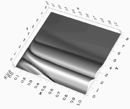
Figure 5: This figure shows a surface plot of $|\psi(\tau,x)|$ for a near-critical evolution. When the initial Gaussian reaches the origin, it is “instantly” (in retarded time $u$) radiated to future null infinity ${\mathscr{I}}^{+}$ (located at $x=1$) by interfering nonlinearly with the field that has not yet reached the origin. Once the evolution has come close to the critical solution, the matter field $\psi(u,x)=\phi r$ decays exponentially; further self-similar features are thus not visible in this plot.

As has become common practice, we find near-critical data through a bisection search in $p$. This procedure yields in particular a numerical approximation to the critical value $p=p*$ which defines the threshold of singularity formation.

In the bisection search, a number of criteria are possible to distinguish dispersion from collapse. Their equivalence can be checked a posteriori when comparing the final result, i.e. subcritical and supercritical solutions close to criticality. A typical criterion is to monitor the ratio $2m/r$, where $2m/r=1$ signifies the presence of an apparent horizon. This criterion has been used successfully also in combination with slicing conditions, that do not penetrate apparent horizons – as is the case in our approach. Numerically, we have used the condition $2m/r\geq 0.995$ as the threshold for apparent horizon formation and for estimating the black hole mass. Remarkably, in practice it turns out, that $2m/r\geq 0.6$ is a sufficient criterion to mark a scalar field evolution as supercritical and thus is useful to speed up bisection searches. For practical and historical reasons, this is the approach we have adopted for our code.

A number of other options come to mind, in particular in our context of evolving out to null infinity, one could e.g. monitor the redshift or Bondi mass. In a dispersion evolution, the redshift will decay to zero, while it will approach infinity when a black hole forms. Similarly, the Bondi mass will decay to zero with a characteristic tail behavior, as is shown in Fig. 6, in a dispersion evolution, and will asymptote to a (positive) constant when the field does not disperse.

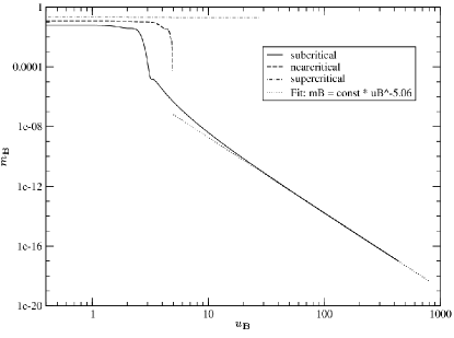
Figure 6: We compare the decay of the Bondi mass in supercritical, near–critical and subcritical evolutions. In the subcritical case, the Bondi mass is found to decay for late times with a power-law exponent of approximately $-5$.

In the course of a near-critical evolution, remnants of the self-similar dynamics which occur locally, inside the SSH, are radiated to future null infinty. Remarkably, we observe that the imprints of DSS behavior are still present in asymptotic quantities such as the Bondi mass and the news function (see figures 7 and 8).

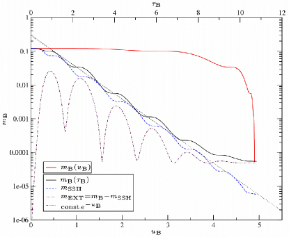
Figure 7: This figure plots the Bondi mass $m_{\scriptscriptstyle\text{B}}$ against both $u_{\scriptscriptstyle\text{B}}$ and the adapted time $\tau_{\scriptscriptstyle\text{B}}$ for a barely supercritical evolution with final black hole mass $M_{f}\approx 5\times 10^{-6}$. The Bondi mass $m_{\scriptscriptstyle\text{B}}$ and the mass at the past SSH, $m_{\scriptscriptstyle\text{SSH}}$, are found to decrease exponentially in $\tau_{\scriptscriptstyle\text{B}}$ (with an overlayed $\tau_{\scriptscriptstyle\text{B}}$-periodic oscillation with period $\Delta/2$), once the evolution has sufficiently approached the critical solution near the center of spherical symmetry. We also show $m_{\scriptscriptstyle\text{EXT}}$, the energy present outside of the SSH.

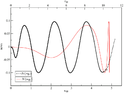
Figure 8: We show the news function $N(u)$, first as a function of the natural time coordinate $u_{\scriptscriptstyle\text{B}}$ of an asymptotic observer and also as a function of a suitably adapted time $\tau_{\scriptscriptstyle\text{B}}=-\ln\frac{u_{\scriptscriptstyle\text{B}}^{*}-u_{\scriptscriptstyle\text{B}}}{u_{\scriptscriptstyle\text{B}}}$ where $N(\tau_{\scriptscriptstyle\text{B}})$ is periodic with period $\Delta\simeq 3.44$ after the spacetime has come close to the critical solution. Even if the constant $u_{\scriptscriptstyle\text{B}}^{*}$ is not known, it can be determined by a fit to periodicity in $\tau_{\scriptscriptstyle\text{B}}$. Thus, it is possible to observe DSS at ${\mathscr{I}}^{+}$ and to extract the critical exponent $\Delta$.

In addition, in numerical evolutions of supercritical data, the black hole mass has been found to exhibit a universal scaling law (see Hod and Piran (1997); Koike et al. (1995); Gundlach (1997a)):

$$\ln m_{\scriptscriptstyle\text{BH}}=\gamma\ln(p-p^{*})+\Psi(\ln(p-p^{*}))+const,$$ (32)

where $\gamma\approx 0.373$ and the function $\Psi$ is periodic with period $\frac{1}{2}\Delta/\gamma$ in $\ln(p-p^{*})$. One needs to ensure to measure the mass of the outermost component of the horizon in order to obtain the fine-structure of the scaling law shown in figure 9.

\psfrag{'masses' using (lp($1)):(log($5) - 0.373*lp($1) +0.74)}{}\includegraphics[angle={-90},clip,width=216.81pt]{mBH-level-fine-structure.ps}

Figure 9: The fine-structure in $m_{\scriptscriptstyle\text{BH}}$ after subtracting a linear fit. The measured period $4.6$ is close to the value predicted by perturbation theory $\frac{1}{2}\Delta/\gamma\approx 4.61$.

This scaling law has been derived by arguments based on linear perturbation theory around the critical solution and dimensional analysis however without using a precise definition of the black hole mass Hod and Piran (1997); Gundlach (1997a). A typical approach in numerical simulations based on coordinates that do not penetrate apparent horizons, as far as we are aware, is to follow a peak in $2m/r$ until this quantity almost reaches unity, at which point the simulation is usually slowed down by a Courant-Friedrichs-Levy (CFL)-type condition, and then read off the approximate horizon mass at this point. We follow this heuristic approach, and are able to reproduce the mass scaling and fine structure.

At least conceptually, this approach is problematic without quantifying how much mass-energy still remains outside of the peak in $2m/r$ where the horizon-mass is read off. From the perturbation theory argument, one expects scaling behavior only for quantities within the self-similar region of spacetime, which does not necessarily extend beyond the SSH. We will return to this point in the discussion section V.

Note that for a near-critical solution, the approximate value of the accumulation time naturally defines an approximate location (i.e. advanced time) of the SSH.

For observers at null infinity, a natural time coordinate is Bondi time $u_{\scriptscriptstyle\text{B}}$ as defined in eq. (16) – Bondi time can be identified with the proper time of timelike observers at large distances – see the discussion in Sec. V. In order to analyze critical phenomena, we define a time coordinate which is suitably adapted to self-similar critical collapse and set

$$\tau_{\scriptscriptstyle\text{B}}=-\ln\frac{u_{\scriptscriptstyle\text{B}}^{*}-u_{\scriptscriptstyle\text{B}}}{u_{\scriptscriptstyle\text{B}}}.$$ (33)

The adapted time coordinate $\tau_{\scriptscriptstyle\text{B}}$ can be defined for spacetimes which are close to the critical solution inside of the SSH, so that the value of the accumulation time $u_{\scriptscriptstyle\text{B}}^{*}$ can be determined by a fit to periodicity in $\tau_{\scriptscriptstyle\text{B}}$. We have used a fit to periodicity of the news function – $N(\tau_{\scriptscriptstyle\text{B}})$ is periodic with period $\Delta\simeq 3.44$ after the spacetime has come close to the critical solution (see figure 8).

Note that $\tau_{\scriptscriptstyle\text{B}}$ is only an approximate adapted coordinate since it depends on the relation between Bondi and central time (16). In order to gain some insight into the behavior of $\tau_{\scriptscriptstyle\text{B}}(\tau)$ consider the simpler case of a continuously self-similar (CSS) collapse. We assume that $\beta$ changes only little outside the past SSH, i.e. $H(u)\approx\beta_{\scriptscriptstyle\text{SSH}}(u)$. Then, since $\beta_{\scriptscriptstyle\text{SSH}}(u)=constant$ in the CSS regime, we find by integrating (16) that

$$u_{\scriptscriptstyle\text{B}}\approx Cu,$$ (34)

where $C=e^{2\beta_{\scriptscriptstyle\text{SSH}}}$ and we have chosen the initial condition $u_{\scriptscriptstyle\text{B}}(0)=0$. Furthermore, it follows from the definition of the adapted time coordinates, equations (9) and (33), that

$$\tau_{\scriptscriptstyle\text{B}}\approx\tau,$$ (35)

in the CSS regime. Numerically, the deviations from this relation for the DSS case turn out to be quite small.

IV.2 DSS behavior in the Bondi Mass and the News Function

The following argument suggests that the news function is approximately periodic in $\tau_{\scriptscriptstyle\text{B}}$, as shown in figure 8. Assume effective DSS data for the scalar field and the metric functions on the past self-similarity horizon (SSH) (see figure 10). Moreover, we assume that the contribution of the right hand side integral in the wave equation for the scalar field (24) can be neglected outside of the SSH, such that the DSS data on the SSH are linearly propagated to ${\mathscr{I}}^{+}$ without backscattering, i.e.

$$\lim_{r\to\infty}\psi(u,r)\approx\psi_{\scriptscriptstyle\text{SSH}}(u).$$ (36)

Furthermore, assume that changes in $\beta$ outside of the SSH are small, so that $\beta_{\scriptscriptstyle\text{SSH}}(u)\approx H(u)$. It then follows that

$$\begin{split}N(u_{\scriptscriptstyle\text{B}})&=\frac{dc(u_{\scriptscriptstyle\text{B}})}{du_{\scriptscriptstyle\text{B}}}\approx\frac{d\psi_{\scriptscriptstyle\text{SSH}}(u)}{du_{\scriptscriptstyle\text{B}}}\\ &=\frac{d}{d\tau}\Bigl{[}\phi_{\scriptscriptstyle\text{SSH}}(\tau)\zeta(\tau)e^{-\tau}u^{*}\Bigr{]}\frac{e^{\tau}}{u^{*}}e^{-2H}\\ &=e^{-2\beta_{\scriptscriptstyle\text{SSH}}}\Bigl{[}\frac{d}{d\tau}\left(\phi_{\scriptscriptstyle\text{SSH}}(\tau)\zeta(\tau)\right)-\phi_{\scriptscriptstyle\text{SSH}}(\tau)\zeta(\tau)\Bigr{]},\end{split}$$ (37)

which shows that the news function $N(u_{\scriptscriptstyle\text{B}})$ is approximately periodic in $\tau$ (and in $\tau_{\scriptscriptstyle\text{B}}$ if equation (35) holds) with period $\Delta$ and satisfies $N(\tau+n\Delta/2)=(-1)^{n}N(\tau)$.

\psfrag{Scri+}{$\scriptstyle{\mathscr{I}}^{+}$}\psfrag{r=0}{$\scriptstyle z=0$}\psfrag{past SSH}{\scriptsize past SSH}\psfrag{z=1}{$\scriptstyle z=1$}\psfrag{future SSH}{\scriptsize future SSH}\psfrag{z=infty}{$\scriptstyle z=\infty,\tau=\infty$}\psfrag{tau=const}{$\scriptstyle\tau=const$}\includegraphics[clip,width=130.08731pt]{SSH.eps}

Figure 10: A conformal diagram of a critical collapse spacetime. In the backwards light cone of the accumulation point the dynamics are close to the DSS critical solution. The lightlike boundary is also called the past self-similarity horizon (SSH). Depending on whether the initial data are sub- or supercritical, the spacetime will for late times be Minkowski or Schwarzschild.

In order to determine the behavior of the Bondi mass, we can then rewrite the Bondi mass-loss equation (17)

$$\frac{dm_{\scriptscriptstyle\text{B}}}{d\tau_{\scriptscriptstyle\text{B}}}=-4\pi N^{2}(\tau_{\scriptscriptstyle\text{B}})\frac{du_{\scriptscriptstyle\text{B}}}{d\tau_{\scriptscriptstyle\text{B}}}=-4\pi u_{\scriptscriptstyle\text{B}}^{*}e^{-\tau_{\scriptscriptstyle\text{B}}}N^{2}(\tau_{\scriptscriptstyle\text{B}}).$$ (38)

Since $N^{2}(\tau_{\scriptscriptstyle\text{B}})$ is $\Delta/2$-periodic in $\tau_{\scriptscriptstyle\text{B}}$, $m_{\scriptscriptstyle\text{B}}$ then takes the following form

$$m_{\scriptscriptstyle\text{B}}(\tau_{\scriptscriptstyle\text{B}})\approx e^{-\tau_{\scriptscriptstyle\text{B}}}f_{\scriptscriptstyle\text{SSH}}(\tau_{\scriptscriptstyle\text{B}}),$$ (39)

where $f_{\scriptscriptstyle\text{SSH}}(\tau_{\scriptscriptstyle\text{B}})$ is $\Delta/2$-periodic in $\tau_{\scriptscriptstyle\text{B}}$.

This behavior mimics the behavior of the mass-function: We rewrite the mass-function in adapted coordinates $(\tau,z)$, using (10),

$$m(\tau,z)=\frac{1}{2}ze^{-\tau}\zeta(\tau)u^{*}\Bigl{[}1-\frac{V}{r}(z,\tau)e^{-2\beta(z,\tau)}\Bigr{]},$$ (40)

and evaluate it at the SSH, which, by a judicious choice of the periodic function $\zeta(\tau)$ can be chosen to be at $z=1$ (since the past SSH is a null surface, one needs to ensure that $\nabla_{a}z$ becomes null at $z=1$). We obtain

$$m_{\scriptscriptstyle\text{SSH}}(\tau)=e^{-\tau}f^{*}_{\scriptscriptstyle\text{SSH}}(\tau),$$ (41)

where $f^{*}_{\scriptscriptstyle\text{SSH}}(\tau)$ is periodic with period $\Delta/2$.

The periodicity and exponential decay of $m_{\scriptscriptstyle\text{B}}$ and $m_{\scriptscriptstyle\text{SSH}}$ are confirmed by our numerical calculations (see fig. 7). Note that the Bondi mass levels off at roughly $10^{-4}$ of the mass in the initial configuration, whereas the mass contained within the backwards light cone $m_{\scriptscriptstyle\text{SSH}}$ continues to scale according to the prediction of critical collapse evolution, equation (39). Since the difference, i.e. $m_{\scriptscriptstyle\text{EXT}}=m_{\scriptscriptstyle\text{B}}-m_{\scriptscriptstyle\text{SSH}}$, is almost zero at the initial slice, we conjecture that $m_{\scriptscriptstyle\text{EXT}}$ is the energy due to backscattering in a critical evolution.

Note that $m_{\scriptscriptstyle\text{EXT}}$ oscillates with $\tau$, as can be seen by integrating

$$\frac{\partial m}{\partial r}=2\pi r^{2}\bigl{(}1-\frac{2m}{r}\bigr{)}\left(\frac{\partial\phi}{\partial r}\right)^{2},$$ (42)

from the SSH to ${\mathscr{I}}^{+}$. The biggest contribution to $m_{\scriptscriptstyle\text{EXT}}$ will come from the vicinity of the past SSH.

We observe that $m_{\scriptscriptstyle\text{EXT}}$ contained in a slice close to horizon formation is almost constant for different near critical evolutions (down to the numerical limit of fine tuning). Therefore, if this $m_{\scriptscriptstyle\text{EXT}}$ eventually falls through the horizon, then the resulting black hole will have a tiny but finite Bondi mass, no matter how fine tuned the data are . In the very late stages of the evolution, the growing redshift, $\beta\to\infty$ effectively halts the numerical evolution, while the error norm $\max|\mathbf{E_{uur}}(\tau_{\scriptscriptstyle\text{B}}>10)|$ approaches $10^{-1}$.

IV.3 Quasinormal Modes

In gravity, quasinormal modes (see Kokkotas and Schmidt (1999) for a review) are excitations of a black hole (or a star) satisfying radiation boundary conditions. These excitations are, in general, obtained from linear perturbations off a fixed background, together with their associated (complex) eigenvalues. Thus, in a highly dynamical setting, such as in critical collapse evolutions, one would not expect to see (identify) quasinormal modes. However, it turns out that for our setting, the least damped spherically symmetric mode for scalar perturbations of a Schwarzschild black hole plays a relevant role.

Perturbation theoryIyer (1987) gives the following value for the half-period

$$\frac{T_{0}}{2}\approx 28.43M_{bg}.$$ (43)

This mode has previously been detected in supercritical evolutions (far away from criticality) for a self-gravitating massless scalar field by Gundlach et al. Gundlach et al. (1994a).

In the following, we analyze radiation signals for near-critical evolutions, where the notion of a fixed background mass does no longer apply. We find that the monopole moment of the scalar field $c(u_{\scriptscriptstyle\text{B}})$ shows a damped oscillation with exponentially decreasing frequency (see figure 11). Moreover, the sizes of the half-periods measured from one extremum to the next in $c(u_{\scriptscriptstyle\text{B}})$ roughly agree with the half-periods obtained from the least damped quasi-normal mode (QNM) of a Schwarzschild black hole with a strongly changing “background” mass $M_{bg}(u_{\scriptscriptstyle\text{B}})$ as shown in figure 12. $M_{bg}(u_{\scriptscriptstyle\text{B}})$ is obtained by evaluating $m_{\scriptscriptstyle\text{B}}(u_{\scriptscriptstyle\text{B}})$ at the mean value between the extrema of $c(u_{\scriptscriptstyle\text{B}})$ (which are inflection points of $m_{\scriptscriptstyle\text{B}}(u_{\scriptscriptstyle\text{B}})$).

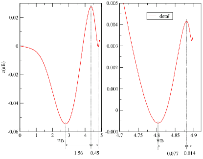
Figure 11: This figure shows the scalar field monopole moment $c(u_{\scriptscriptstyle\text{B}})$ for a near-critical (but barely supercritical) evolution. The half-periods measured from one extremum to the next roughly agree with the prediction of perturbation theory shown in figure 12.

\psfrag{tau_B}{$\scriptstyle\tau_{\scriptscriptstyle\text{B}}$}\psfrag{T0/2(u_B)}{$\scriptstyle T_{0}/2(u_{\scriptscriptstyle\text{B}})$}\psfrag{T0/2 = 28.43 * m_B}[0.9]{$\scriptstyle T_{0}/2\,=\,28.43\,m_{\scriptscriptstyle\text{B}}$}\includegraphics[clip,width=216.81pt]{T0-annotated.eps}

Figure 12: The exponential decay of the QNM half-periods predicted by perturbation theory is shown with annotated values at the midpoints between the points of inflection for the same near–critical evolution as in figure 11.

IV.4 Power-law Tails

As has been established by Price Price (1972), perturbation fields outside of Schwarzschild black holes die off with an inverse power-law tail at late times. In contrast to quasinormal modes this behavior does not depend on the details of the collapse process, but only on the asymptotic falloff of the effective potential; (i.e. in a curved spacetime, wave propagation is not confined to the light cones, rather waves spread inside the light cones, due to scattering off spacetime curvature.) Therefore, tail phenomena can be observed independently of the endstate of the evolution. For Gaussian initial data the Newman-Penrose constant Gómez et al. (1994) vanishes and for late times perturbation theory Gundlach et al. (1994b, a) predicts that the field falls off as $\phi\propto u_{\scriptscriptstyle\text{B}}^{-2}$ near ${\mathscr{I}}^{+}$ and $\phi\propto u_{\scriptscriptstyle\text{B}}^{-3}$ near timelike infinity $i^{+}$.

To be more precise Barack (1999a, b), consider a distant static observer at $r=const$ and Bondi time $\Delta u_{\scriptscriptstyle\text{B}}$ elapsed since the “main pulse” of radiation has reached the observer (the duration of the main pulse has been assumed negligible in Barack (1999a, b)). Null infinity is then found to be approximated by the region where $\Delta u_{\scriptscriptstyle\text{B}}\ll r$ within the context of a perturbative analysis of tail behavior Leaver (1986a, b); Barack (1999a). This regime has been termed the “astrophysical zone” by Leaver Leaver (1986a, b); Barack (1999a).

In addition, the convergence of the perturbation expansion in Barack (1999a, b) requires $\Delta u_{\scriptscriptstyle\text{B}}\gg M$, where $M$ is the mass of the background. In our case, the mass which gives rise to the effective potential is bounded from above by the mass of the initial (ingoing) pulse, $M_{i}$. Therefore, we demand that $\Delta u_{\scriptscriptstyle\text{B}}\gg M_{i}$. Numerically, we observe tails only for $\Delta u_{\scriptscriptstyle\text{B}}>10^{3}M_{i}$.

Closeness to timelike infinity, on the other hand, demands $\Delta u_{\scriptscriptstyle\text{B}}\gg|r_{*}|$, where $r*$ is the usual “tortoise” coordinate $r_{*}=r+2M\ln\bigl{(}\frac{r-2M}{2M}\bigr{)}$. In figure 13 we show power-law exponents determined by fits of $\psi$ at different $r=const$ curves over a series of time intervals for a subcritical evolution. As described in section III we use spline interpolation to calculate $\psi(x=const)$. The exponents have been determined by fitting the field $\psi$ at $x=constant$ against a power of $u_{\scriptscriptstyle\text{B}}$ in 5 distinct time intervals of the evolution. The domains of validity of the exponents predicted by perturbation theory, $-2$ near ${\mathscr{I}}^{+}$ and $-3$ near $i^{+}$, can be observed here. It is clear that the outermost gridpoints in this evolution (using 10000 gridpoints) are indeed located in the “astrophysical zone” since $r(x=0.9995)\approx 2000\gg\Delta u_{\scriptscriptstyle\text{B}}$, where $\Delta u_{\scriptscriptstyle\text{B}}$ is the Bondi time elapsed since the main pulse of radiation has reached the observer at about $u_{\scriptscriptstyle\text{B}}\approx 3$ (see figure 6). On the other hand, closeness to timelike infinity $i^{+}$ demands that $\Delta u_{\scriptscriptstyle\text{B}}\gg r_{*}$. Note that $r_{*}\approx r$ for $r\gg 2M_{i}$, where $M_{i}\approx 0.06$ is the initial Bondi mass. It is also apparent that for $\Delta u_{\scriptscriptstyle\text{B}}\approx r$ the observers are in between the two zones and the power-law exponents seem to change smoothly.

\psfrag{uB}{$\scriptstyle u_{\scriptscriptstyle\text{B}}$}\includegraphics[clip,width=260.17464pt]{tails-reg.eps}

Figure 13: This figure shows power-law exponents for a subcritical evolution and illustrates the domains of validity of the predictions of perturbation theory for the two zones: $-2$ near ${\mathscr{I}}^{+}$ and $-3$ near $i^{+}$.

Figure 6 displays the power-law decay, with exponent $-5$, of the Bondi mass for the same subcritical evolution. This behavior can be explained by integrating the Bondi mass-loss equation (17) with $c\propto u_{\scriptscriptstyle\text{B}}^{-2}$ in the regime of power-law tails.

Note that in situations involving realistic sources and realistic detectors, power-law tails only play a minor (if any) role as an actual signal, but the power-law tail results still can provide hints on how to resolve the very important question of whether null infinity is a useful idealisation for gravitational wave detectors. Accordingly, we suggest to generalize the term “astrophysical zone” to more general, non-perturbative situations, by reinterpreting – in a very loose sense – $\Delta u_{\scriptscriptstyle\text{B}}$ as a suitably chosen large time scale characteristic of the source. The physical idea is that the distance from observers of astrophysical phenomena, e.g. gravitational wave detectors, to the radiation sources is very large compared to the time during which substantial radiation from the source can be observed. This is at least expected for sources where general relativity is important, as opposed to problems for which a (Post-) Newtonian approach and the quadrupole formula are sufficient. An example would be a binary black hole merger in another galaxy, which might have a characteristic dynamical time scale of a fraction of a second, and which might be observed during several thousand cycles, including a portion of the QNM ringdown.

V Discussion

In this work we have presented numerical constructions of portions of near-critical spherically symmetric spacetimes that extend up to future null infinity and asymptote to the event horizon. The simulations are based on a compactified approach, where the equations have been regularized in a neighborhood of null infinity by introducing the mass function as an additional independent variable. The resolution necessary to resolve critical phenomena is gained through letting our gridpoints fall along ingoing null geodesics, following Garfinkle Garfinkle (1995). The grid is repopulated with grid points, which are filled with values through interpolations when half of the gridpoints have reached the origin. This is not optimal, but ensures sufficient resolution for our current purposes.

We reproduce standard features of near-critical solutions, such as “echoing” and mass scaling with fine structure. In addition we extract radiation at null infinity by computing the news function and find a signal with rapidly increasing frequency as measured in Bondi time, which is the natural time coordinate associated with far away observers. In order to simplify the analysis of near-critical spacetimes, we have defined an approximate adapted time in terms of Bondi time, in analogy to the standard time coordinate which is adapted to the DSS discrete diffeomorphism (3). This coordinate can be used by asymptotic observers to render the signal from a near-critical collapse (almost) periodic. The fact that such a definition actually works out, and makes DSS periodicity manifest in quantities defined at null infinity is a non-trivial result, which we explain in Sec. IV.1.

Note also that the amplitude of the news function, shown in Fig. 8 stays fairly constant after the initial transient. This feature is clearly universal, as long as the radiation signal is dominated by the DSS collapse, since the system can be approximated in the DSS region by a perturbation of the critical solution, and, according to our results, the radiation signal is dominated by the DSS structure of the critical solution. Thus, in section IV.2, we neglect contributions from scalar field which is far outside the DSS region and does not contribute to the critical collapse dynamics. Consequently, in this scenario the essential free parameters determining the radiation signal from an actual near critical solution are the number of cycles the solution spends in the neighborhood of the critical solution and the length scale at which the solution comes close to the critical solution. The robustness of this scenario, i.e. what happens if the initial data are such that there is significant mass outside of the SSH, is outside of the scope of this paper and an issue for future research.

Perhaps the most surprising feature of the radiation signal has emerged from our investigation of QNM’s, which has been motivated by Gundlach et al. (1994a), where the first quasinormal mode is found in collapse evolutions and the question is posed as to how QN ringing would change close to criticality. We find that even in very close-to-critical evolutions there is a correlation of the radiation signal with the period of the first quasinormal mode, determined from the time-dependent value of the Bondi mass, as disussed in Sec. IV.3, Figs. 11 and 12. This correlation between the radiation of the highly dynamical near-critical solution and the quasinormal mode, that is defined in terms of perturbations of a static spacetime, certainly deserves further investigation. This surprising feature might even turn out to be a key toward understanding the phenomenon of DSS behaviour in near-critical spacetimes. Our results seem to suggest that the effective curvature potential for a DSS self-gravitating field acts as a quasi-stationary background for scattering processes which can be approximately described by quasinormal modes of a 1-parameter family of Schwarzschild black holes with exponentially decreasing mass. The question of the applicability of QNM-motivated estimates is quite relevant for numerical relativity, e.g. when extracting wave forms from binary mergers. In the very different context of quasinormal modes of Schwarzschild-AdS black holes, Horowitz and Hubeny Horowitz and Hubeny (2000) have pointed out an agreement of the numerical values of the critical exponent and the imaginary part of quasinormal frequencies, and have speculated on a connection between critical collapse and quasinormal modes. While Horowitz and Hubeny assume pure coincidence as the most likely explanation, it seems worth to keep in mind in future work concerning critical collapse or quasinormal modes.

For subcritical initial data we can evolve for very long times, and thus are able to observe power-law tail behavior as shown in Figs. 13 and 6. Analytical calculations predict different falloff rates for radiation along null infinity and along timelike lines, and the natural question arises, which falloff rate would be seen by a hypothetical observer (in a realistic case, observation of power-law tails would require an extremely large signal-to-noise ratio). Accordingly, our results depicted in Fig. 13 show how the rates at finite but large radius correspond to the value for null infinity for a while before they approach the expected late-time value for finite radius. The interpretation of this phenomenon is suggested by perturbative work of Barack (1999a, b), where different tail falloff rates are computed. There, different regions of spacetime are identified, where certain approximations hold. Within the perturbative regime, results obtained for null infinity are valid for what has been termed the “astrophysical zone” by Leaver Leaver (1986a, b); Barack (1999a), and which is defined as the region where $\Delta u_{\scriptscriptstyle\text{B}}\ll r$. (Note, however, that $u_{\scriptscriptstyle\text{B}}\gg M$ must also be satisfied). The physical idea is that the distance from observers of astrophysical phenomena, e.g. gravitational wave detectors, to the radiation sources is very large compared to the time during which the source radiates at an observable rate.

We argue that our results illustrate that the relevant falloff from the point of view of an astrophysical observer is the falloff rate at null infinity, in accordance with the prediction from perturbation theory. We believe that this is a nice model calculation that exemplifies that null infinity is indeed a useful approximation for observers at large distance from the source, in the sense that such observers are located in the “astrophysical zone”.

Along the same lines, we would like to point out that by taking appropriate limits in a conformally compactified manifold, worldlines of increasingly distant geodesic observers converge to null geodesic generators of future null infinity and proper time converges to Bondi time Frauendiener (2000). Note also that a naive correspondence between observers at large distance and spatial infinity would be problematic, e.g. compactification at spatial infinity leads to “piling up” of waves, whereas at null infinity this effect does not appear – waves leave the physical spacetime through the boundary at null infinity.

Under practical circumstances, e.g. computing the signal from a source of radiation which is locted at a cosmological distance from the detector, null infinity more realistically corresponds to an observer that is sufficiently far away from the source to treat the radiation linearly, but not so far away that cosmological effects have to be taken into account. We are however not aware of a discussion where this sloppy picture has been made more precise.

When looking at critical collapse from a global spacetime perspective, as we have done here, one is confronted with some issues concerning the mass-scaling, that we would like to comment on briefly: When asking the question of whether infinitesimally small black holes can be formed – the question which triggered the original work on critical collapse – it could be phrased in two slightly different ways: (i) can we form black-hole solutions where the final-state black hole has arbitrarily small mass, or (ii) can we form arbitrarily small apparent horizons. The question which has been aswered in the affirmative by critical collapse research is the second one. The first one still seems open. Our results for near-supercritical evolutions seem to indicate that the final black hole is significantly larger than the mass leading to scaling. We conjecture that due to backscattering of the outgoing radiation one cannot form arbitrarily small black holes, no matter how fine tuned the data are.

Finally, we want to emphasize the obvious fact that the failure of the critical solution to be asymptotically flat is perfectly consistent with its role in the dynamics of a localized object emitting radiation to null infinity. First, note that for the dynamics of critical collapse, only a small region of spacetime is relevant. The scale-invariance of the DSS solution is compatible with asymptotic flatness in the following way: a near critical solution, which may or may not be asymptotically flat, comes close to the critical solution at a length scale which depends on the initial data, follows the critical solution for a number of cycles, and then collapses or disperses. The (discrete) self-similarity of the critical solution is on the one hand responsible for the failure of the critical solution to be asymptotically flat but actually makes it possible to keep a free length scale in the problem of massless scalar field collapse, as is expected to allow for asymptotically flat near critical solutions.