5-dimensional Brans-Dicke Theory and Cosmic Acceleration

Abstract

We consider a 5-dimensional scalar-tensor theory which is a direct generalization of the original 4-dimensional Brans-Dicke theory to 5-dimensions. By assuming that there is a hypersurface-orthogonal spacelike Killing vector field in the underlying 5-dimensional spacetime, the theory is reduced to a 4-dimensional theory where the 4-metric is coupled with two scalar fields. The cosmological implication of this reduced theory is then studied in the Robertson-Walker model. It turns out that the two scalar fields may account naturally for the present accelerated expansion of our universe. The observational restriction of the reduced cosmological model is also analyzed.

PACS number(s): 04.50.+h, 98.80.Es

1 Introduction

The observations on the explosion of type Ia supernova indicate that the expansion of our universe might be presently accelerating [1, 2]. The main component of the universe responsible for the acceleration is usually called as dark energy, which constitutes about three fourths of the whole matter budget of our universe according to the recent WMAP date [3]. There are a number of quintessence models of dark energy, which have been put forward and most of them involve minimally coupled scalar field with different potentials [4, 5, 6]. In order to extract a potential suitable for describing the universe, two-field quintessence model have also been taken account [7, 8]. Further models, such as (generalized) chaplygin gas [9, 10] and K-essence [11, 12], are proposed to account for both dark energy and dark matter in a unified way. However, in all these phenomenological models, the scalar fields are added by hand and hence their origins are yet understood. To explain the accelerated expansion of the universe from fundamental physics is now a great challenge. Some researchers resort to Brans-Dicke theory [13, 14], which is a modified relativistic theory of gravitation apparently compatible with Mach’s principle [15]. The scalar field in Brans-Dicke theory is then expected to account for the desired quintessence or K-essence. However, the scalar field can naturally lead to cosmological acceleration only when the coupling parameter $\omega$ varies with time [13] or there is a potential for it added by hand [14]. On the other hand, the models of accelerating universe leading by dynamical compactification of extra dimensions in Kaluza-Klein theory are also proposed [16, 17]. As a candidate of fundamental theory, Kaluza-Klein theory unifies gravity with electromagnetic field (or Yang-Mill field) by certain higher dimensional general relativity [18, 19]. It is reasonable to propose a fundamental theory which combines the advantages of both Brans-Dicke and Kaluza-Klein. We thus consider higher dimensional Brans-Dicke theories [20] as available candidates.

In this paper, to illustrate the physics of these theories we generalize Brans-Dicke theory to 5 dimensions and study its effect in the 4-dimensional sensational world. On the assumption that there is a hypersurface-orthogonal spacelike Killing vector field in the underlying 5-dimensional spacetime, the theory is reduced to a 4-dimensional theory where the 4-metric is coupled with two scalar fields. Note that if the extra dimension is compactified as a circle $S^{1}$ with a microscopic radius, a Killing vector field may arise naturally in low energy regime[19]. The cosmological implication of this reduced theory is then studied in the Robertson-Walker model. Numerical analysis shows that the two scalar fields can be used to account for the present expansion of our universe, while current observations impose crucial restrictions on the admissible range of the free parameters in the reduced model.

2 Killing reduction of 5-dimensional Brans-Dicke theory

Killing reduction of 4-dimensional and 5-dimensional spacetimes have been studied by Geroch[21] and Yang et.al.[22]. Let ($M,g_{ab}$) be an $n$-dimensional spacetime with a Killing vector field $\xi^{a}$, which is everywhere spacelike. Let $S$ denote the collection of all trajectories of $\xi^{a}$. There is a one-to-one correspondence between tensor fields $\hat{T}_{a...c}^{b...d}$ on $S$ and tensor fields $T_{a...c}^{b...d}$ on $M$ which satisfy

$$\begin{array}[]{l}\xi^{a}T^{b\cdots d}_{a\cdots c}=0,\ \cdots\ ,\xi_{d}T^{b\cdots d}_{a\cdots c}=0,\\ {\mathcal{L}}_{\xi}T^{b\cdots d}_{a\cdots c}=0,\end{array}$$ (1)

where ${\mathcal{L}}_{\xi}$ denotes the Lie derivative with respect to $\xi^{a}$. Note that the abstract index notation [23] is employed. The entire tensor field algebra on $S$ is completely and uniquely mirrored by tensor field on $M$ subject to Eq.(1). Thus, we shall speak of tensor fields being on $S$ merely as a shorthand way of saying that the fields on $M$ satisfy Eq.(1). The metric on $S$ is defined as $h_{ab}=g_{ab}-\lambda^{-1}\xi_{a}\xi_{b}$, where $\lambda\equiv\xi^{a}\xi_{a}$.

The action of our 5-dimensional Brans-Dicke theory is proposed as

$$S_{5}=\int d^{5}x\sqrt{-g}[\phi R^{(5)}-\frac{\omega}{\phi}g^{ab}(\nabla_{a}\phi)\nabla_{b}\phi]+\frac{16\pi}{c^{4}}\int d^{5}x\sqrt{-g}L_{m}^{(5)},$$ (2)

where $R^{(5)}$ is the curvature scalar associated with the 5-dimensional space-time metric $g_{ab}$, $\phi$ is a scalar field, $\omega$ is a coupling constant, and $L_{m}^{(5)}$ represents the 5-dimensional Lagrangian of the matter fields. The field equation of $g_{ab}$ derived from $(\ref{s5})$ reads

$$G_{ab}^{(5)}=\frac{8\pi\phi^{-1}}{c^{4}}T_{ab}^{(5)}+\frac{\omega}{\phi^{2}}[(\nabla_{a}\phi)\nabla_{b}\phi-\frac{1}{2}g_{ab}(\nabla^{c}\phi)\nabla_{c}\phi]+\phi^{-1}(\nabla_{a}\nabla_{b}\phi-g_{ab}\nabla^{c}\nabla_{c}\phi),$$ (3)

where $G_{ab}^{(5)}$ is the 5-dimensional Einstein tensor, and $T_{ab}^{(5)}$ represents the 5-dimensional energy momentum tensor of matter field with trace $T^{(5)}=T_{ab}^{(5)}g^{ab}$. While the field equation of $\phi$ is determined by (2) as

$$\nabla^{a}\nabla_{a}\phi=\frac{8\pi}{c^{4}}\frac{T^{(5)}}{4+3\omega}.$$ (4)

We restrict ourselves to 5-dimionsional Brans-Dicke spacetime with a Killing vector field $\xi^{a}$, which preserves both $g_{ab}$ and $\phi$ and is everywhere spacelike. Without lose generality we choose a coordinate system $\{x^{\mu},x^{5}\},\mu=0,1,2,3,$ adapted to the congruence of $\xi^{a}$, i.e., $(\frac{\partial}{\partial x^{5}})^{a}=\xi^{a}$. In the case where $\xi^{a}$ is not hypersurface-orthogonal, $\xi_{\mu}\neq 0$, $\xi_{\mu}$ will behave as the electromagnetic 4-potential in the reduced 4-dimensional theory. Since we concern mainly on the effect of the reduced scalar fields, to simplify the discussion, we will consider only the case where $\xi^{a}$ is hypersurface-orthogonal. Then the line element of $g_{ab}$ reads $ds^{2}=g_{\mu\nu}dx^{\mu}dx^{\nu}+\lambda dx^{5}dx^{5}$. Through Killing reduction, the Ricci tensor $R^{(4)}_{ab}$ of the 4-metric $h_{ab}$ and the scalar field $\lambda$ are related to the Ricci tensor $R^{(5)}_{ab}$ of $g_{ab}$ by

$$R_{ab}^{(4)}=\frac{1}{2}\lambda^{-1}D_{a}D_{b}\lambda-\frac{1}{4}\lambda^{-2}(D_{a}\lambda)D_{b}\lambda+h_{a}^{m}h_{b}^{n}R_{mn}^{(5)}$$ (5)

and

$$D^{2}\lambda=\frac{1}{2}\lambda^{-1}(D^{a}\lambda)D_{a}\lambda-2R_{ab}^{(5)}\xi^{a}\xi^{b},$$ (6)

where $D^{2}\equiv D^{a}D_{a}$ and $D_{a}$ is the covariant derivative on $S$ defined by $D_{e}T_{a\ldots c}^{b\ldots d}=h_{e}^{p}h_{a}^{m}\ldots h_{c}^{n}h_{r}^{b}\ldots h_{s}^{d}\nabla_{p}T_{m\ldots n}^{r\ldots s}$, which satisfies all the conditions of a derivative operator.

Let the matter content in Eq.(2) be a 5-dimensional perfect fluid with energy momentum tensor $T_{ab}^{(5)}=(\rho^{(5)}+P^{(5)})U_{a}U_{b}+P^{(5)}g_{ab}$, where $\rho^{(5)}$ and $P^{(5)}$ are the energy density and hydrostatic pressure respectively measured by comoving observers, and $U^{a}$ is the 5-velocity of the fluid. Suppose the fluid does not move along the fifth dimension, then $U_{a}\xi^{a}=0$. In the reduced 4-dimensional spacetime $S$, it looks like a 4-dimensional perfect fluid with energy-momentum: $T_{ab}=(\rho+P)U_{a}U_{b}+Ph_{ab}$, where $\rho\equiv\int\lambda^{\frac{1}{2}}\rho^{(5)}dx^{5}=\lambda^{\frac{1}{2}}L\rho^{(5)}$ and $P\equiv\int\lambda^{\frac{1}{2}}P^{(5)}dx^{5}=\lambda^{\frac{1}{2}}LP^{(5)}$; here $L$ is the coordinate scale of the extra dimension. $T_{ab}^{(5)}$ can then be written into

$$T_{ab}^{(5)}=\frac{1}{L\lambda^{\frac{1}{2}}}[(\rho+P)U_{a}U_{b}+Pg_{ab}].$$ (7)

Substituting Eq. (3) into (5), we obtain the 4-dimensional field equation for $h_{ab}$ as:

$$G_{ab}^{(4)} = \frac{8\pi\phi^{-1}L^{-1}\lambda^{-\frac{1}{2}}}{c^{4}}T_{ab}^{(4)}+\frac{1}{2}\lambda^{-1}(D_{a}D_{b}\lambda-h_{ab}D^{c}D_{c}\lambda)-\frac{1}{4}\lambda^{-2}[(D_{a}\lambda)D_{b}\lambda-h_{ab}(D^{c}\lambda)D_{c}\lambda]$$ (8)

$$+ \frac{\omega}{\phi^{2}}[(D_{a}\phi)D_{b}\phi-\frac{1}{2}h_{ab}(D^{c}\phi)D_{c}\phi]+\phi^{-1}(D_{a}D_{b}\phi-h_{ab}D^{c}D_{c}\phi)-\frac{\phi^{-1}}{2}\lambda^{-1}h_{ab}(D^{c}\lambda)D_{c}\phi.$$

The reduction of Eq. (4) leads to the 4-dimensional field equation of $\phi$ as

$$D^{a}D_{a}\phi=-\frac{1}{2}\lambda^{-1}(D^{c}\lambda)D_{c}\phi+\frac{8\pi L^{-1}\lambda^{\frac{1}{2}}}{c^{4}}(\frac{T^{(4)}+P}{4+3\omega}).$$ (9)

By using Eq. (6), we obtain

$$D^{a}D_{a}\lambda=\frac{1}{2}\lambda^{-1}(D^{a}\lambda)D_{a}\lambda-\phi^{-1}(D^{a}\lambda)D_{a}\phi+\frac{8\pi L^{-1}\lambda^{-\frac{1}{2}}\phi^{-1}}{c^{4}}(\frac{2\omega+2}{4+3\omega}T^{(4)}-\frac{4\omega+6}{4+3\omega}P).$$ (10)

Eqs. (8)-(10) can be regarded as those for a 4-dimensional gravity described by a 4-metric coupled to two scalar fields, which are equivalent to 5-dimensional Brans-Dicke’s field equations. The two scalar fields appear naturally in the theory and will be used to explain the present accelerated expansion of the universe.

3 Reduced Brans-Dicke cosmology

To explore the cosmological implication of the reduced Brans-Dicke theory, we consider the homogeneous and isotropic cosmology with the 4-dimensional Friedman-Robertson-Walker metric:

$$ds^{2}=-dt^{2}+a^{2}(t)[\frac{dr^{2}}{1-kr^{2}}+r^{2}d\Omega^{2}],$$ (11)

where $a(t)$ is the scale factor, and $k$ is the spatial curvature index. The 4-velocity $U^{a}$ of the reduced perfect fluid is required to coincide with that of isotropic observers. Then Eq.(8) is reduced to

$$-3\frac{\dot{a}}{a}\frac{\dot{\phi}}{\phi}-\frac{3}{2}\frac{\dot{a}}{a}\frac{\dot{\lambda}}{\lambda}-\frac{1}{2}\frac{\dot{\lambda}}{\lambda}\frac{\dot{\phi}}{\phi}+\frac{\omega}{2}(\frac{\dot{\phi}}{\phi})^{2}+\frac{8\pi}{c^{2}}L^{-1}\phi^{-1}\lambda^{-\frac{1}{2}}\rho=3(\frac{\dot{a}}{a})^{2}+3\frac{k}{a^{2}}$$ (12)

and

$$\frac{\ddot{\phi}}{\phi}+2\frac{\dot{a}}{a}\frac{\dot{\phi}}{\phi}-\frac{1}{4}({\frac{\dot{\lambda}}{\lambda}})^{2}+\frac{1}{2}\frac{\ddot{\lambda}}{\lambda}+\frac{\dot{a}}{a}\frac{\dot{\lambda}}{\lambda}+\frac{1}{2}\frac{\dot{\lambda}}{\lambda}\frac{\dot{\phi}}{\phi}+\frac{\omega}{2}(\frac{\dot{\phi}}{\phi})^{2}+\frac{8\pi}{c^{2}}L^{-1}\phi^{-1}\lambda^{-\frac{1}{2}}P=-(\frac{2\ddot{a}}{a}+\frac{\dot{a}^{2}+k}{a^{2}}),$$ (13)

where a dot on a letter represents a derivative with respective to the proper time $t$ of the isotropic observers. While, Eqs.(9) and (10) become the wave equations for the scalar fields as

$$\ddot{\phi}=-3\frac{\dot{a}}{a}\dot{\phi}-\frac{1}{2}\frac{\dot{\lambda}}{\lambda}\dot{\phi}+\frac{8\pi}{c^{2}}L^{-1}\lambda^{-\frac{1}{2}}\frac{\rho-4P}{3\omega+4}$$ (14)

and

$$\ddot{\lambda}=-3\frac{\dot{a}}{a}\dot{\lambda}+\frac{1}{2}\frac{(\dot{\lambda})^{2}}{\lambda}-\frac{\dot{\phi}}{\phi}\dot{\lambda}+\frac{8\pi L^{-1}\phi^{-1}\lambda^{\frac{1}{2}}}{c^{2}}(\frac{2\omega+2}{3\omega+4}\rho-\frac{2\omega}{3\omega+4}P).$$ (15)

The effective energy density and pressure of the scalar fields can be read out from Eqs.(12) and (13) as

$$\rho_{s}\equiv\frac{c^{2}L\lambda^{\frac{1}{2}}}{8\pi}[-3\frac{\dot{a}}{a}\dot{\phi}-\frac{3}{2}\frac{\dot{a}}{a}\frac{\dot{\lambda}}{\lambda}\phi-\frac{1}{2}\frac{\dot{\lambda}}{\lambda}\dot{\phi}+\frac{\omega}{2}\frac{(\dot{\phi})^{2}}{\phi}]$$ (16)

and

$$P_{s}\equiv\frac{c^{2}L\lambda^{\frac{1}{2}}}{8\pi}[\ddot{\phi}+2\frac{\dot{a}}{a}\dot{\phi}-\frac{1}{4}({\frac{\dot{\lambda}}{\lambda}})^{2}\phi+\frac{1}{2}\frac{\ddot{\lambda}}{\lambda}\phi+\frac{\dot{a}}{a}\frac{\dot{\lambda}}{\lambda}\phi+\frac{1}{2}\frac{\dot{\lambda}}{\lambda}\dot{\phi}+\frac{\omega}{2}\frac{(\dot{\phi})^{2}}{\phi}].$$ (17)

The scalar fields would play the role of dark energy in the universe, provided the following conditions are satisfied [24]: $-1.3<\frac{P_{s}}{\rho_{s}}<-0.7$ and $P_{s}<0$. From Eqs.(16) and (17), one can suppose that these conditions are very possible to be satisfied in certain epoch in the evolution of the universe. We now show by numerical simulation that there are indeed such solutions with accelerated expansion at the present epoch of the universe. Note that equations (12) and (13) combined with (14) and (15) lead to the matter conservation equation

$$\dot{\rho}+3\frac{\dot{a}}{a}(\rho+P)=0.$$ (18)

Since, except for the dark content, the present epoch of the universe is matter dominated, we put $P=0$ in Eq.(18) and set $\rho=\rho_{0}(a_{0}/a)^{3}$, where $\rho_{0}$ is the current value of the energy density of visible matter. Thus we suppose that the dark matter constituent is also involved in the two scalar fields. From Eqs.(12) and (13) we can obtain the evolution equation of the Hubble parameter $H(t)$ as

$$\dot{H}=2\frac{\dot{a}}{a}\frac{\dot{\phi}}{\phi}+\frac{\dot{a}}{a}\frac{\dot{\lambda}}{\lambda}+\frac{1}{2}\frac{\dot{\lambda}}{\lambda}\frac{\dot{\phi}}{\phi}-\frac{\omega}{2}(\frac{\dot{\phi}}{\phi})^{2}-\frac{8\pi}{c^{2}}L^{-1}\lambda^{-\frac{1}{2}}\phi^{-1}\frac{2\omega+3}{3\omega+4}\rho_{0}(\frac{a_{0}}{a})^{3}.$$ (19)

The wave equations (14) and (15) now become

$$\ddot{\phi}=-3\frac{\dot{a}}{a}\dot{\phi}-\frac{1}{2}\frac{\dot{\lambda}}{\lambda}\dot{\phi}+\frac{8\pi}{c^{2}}L^{-1}\lambda^{-\frac{1}{2}}\frac{\rho_{0}}{3\omega+4}(\frac{a_{0}}{a})^{3}$$ (20)

and

$$\ddot{\lambda}=-3\frac{\dot{a}}{a}\dot{\lambda}+\frac{1}{2}\frac{(\dot{\lambda})^{2}}{\lambda}-\frac{\dot{\phi}}{\phi}\dot{\lambda}+\frac{8\pi}{c^{2}}L^{-1}\phi^{-1}\lambda^{\frac{1}{2}}\frac{2\omega+2}{3\omega+4}\rho_{0}(\frac{a_{0}}{a})^{3}.$$ (21)

A necessary and sufficient condition for expansion of the universe to be accelerating is that the deceleration parameter $q\equiv-\frac{a\ddot{a}}{\dot{a}^{2}}$ is negative. Solving Eqs.(19)-(21) by numerical simulation with suitable current observed values as initial values, the evolution of the universe around present epoch can actually be obtained.

The key idea in the dynamical compactification model of Kaluza-Klein cosmology is that the extra dimensions contract while the four visible dimensions expand [20, 16, 17]. We adopt this idea to assume that the present universe satisfies

$$a^{3}(t)\lambda^{\frac{n}{2}}(t)=constant,$$ (22)

where $n$ is a positive number. Then we have

$$\frac{\dot{\lambda}}{\lambda}=-\frac{6}{n}H.$$ (23)

Note that the effective 4-dimensional gravitational parameter in our 5-dimensional theory can be expressed as $G=(\phi\lambda^{\frac{1}{2}}L)^{-1}$. Hence Eq.(23) also implies

$$\frac{\dot{\phi}}{\phi}=\frac{3}{n}H-\frac{\dot{G}}{G}.$$ (24)

Inserting Eqs.(23), (24) and $q=-(1+\dot{H}/H^{2})$ into Eq.(19), we obtain the relation of $\omega$ and $n$ as

$$\omega=\frac{2(1+q-2z-\varrho)n^{2}+6zn-18}{(zn-3)^{2}},$$ (25)

where $z\equiv\dot{G}/GH$ and $\varrho\equiv\frac{8\pi}{c^{2}}G\frac{2\omega+3}{3\omega+4}\rho_{0}(\frac{a_{0}}{a})^{3}H^{-2}$. Taking account of the current observed values $\rho_{0}=(3.8\pm 0.2)\times 10^{-28}kg\cdot m^{-3}$ and $H_{0}=(2.3\pm 0.1)\times 10^{-18}s^{-1}$ [26], we can estimate $\varrho\sim 10^{-18}$. Hence the effect of $\varrho$ in Eq.(25) is so tiny that one can simply neglect it. We thus expect that the current observational range of $q$ and $z$ as well as certain physical consideration would constrain the admissible values of $\omega$ in the 5-dimensional theory and $n$ in the present universe. Taking the current observed values $q_{0}=-0.67\pm 0.25$ [26], $\dot{G}/G=(0.46\pm 1.0)\times 10^{-12}yr^{-1}\cite[cite]{[\@@bibref{}{No}{}{}]}$, and the weak energy condition $\omega\geq-\frac{4}{3}$ [20], numerical simulation do give the restricted range of $\omega$ and $n$ as illustrated in Fig.1. It turns out that the range of $n$ is restricted to $n\geq 2.2$. In general a bigger value of $\omega$ would require a bigger value of $n$. We expect that more astronomical observations, for example the solar system experiments, would further constrain the admissible values of $\omega$ and $n$ [27].

To illustrate the evolutional character of the universe around present epoch in this model, one can choose some particular values of $\omega$ and $n$ in the admissible range and obtain desired evolution curves determined by Eqs.(19)-(21). For example, one may choose $\omega=-1.2$ and $n=3$ together with current initial values $H_{0}=2.3\times 10^{-18}s^{-1}$ and $\rho_{0}=3.8\times 10^{-28}kg\cdot m^{-3}$. Then from Eqs.(23) and (24) one has $(\frac{\dot{\lambda}}{\lambda})_{0}=-4.6\times 10^{-18}s^{-1}$ and $(\frac{\dot{\phi}}{\phi})_{0}=2.3\times 10^{-18}s^{-1}$. Let $a_{0}=1$, $\lambda(t_{0})=1$ and $L=10^{-34}m$, then one gets $\phi(t_{0})=1.5\times 10^{44}kg\cdot m^{-4}\cdot s^{2}$. Taking the above current values as initial values, the evolution of $a(t)$ with $q(t)$, $\phi(t)$ and $\lambda(t)$ are respectively illustrated in Fig.2, Fig.3 and Fig.4. Remarkably, from Fig.2 one can see that the coupling parameter and initial values can be chosen in the allowed range such that the current value of the deceleration parameter reads $q_{0}=-0.60$, which coincides with the current observation. If the age of the universe today is $t_{0}=(13\pm 1.5)Gyr$ [26], the cosmological transition from deceleration to acceleration happens at $t=t_{0}-2.5Gyr$. Fig.3 and Fig.4 show that $\phi(t)$ increases from some small value to a bigger constant while $\lambda(t)$ decreases from some large value to a smaller constant. So both of them are well behaved. Although our cosmological model is yet to be examined, the above result suggests well the scalar fields in higher dimensional Brans-Dicke theories to be responsible for the present cosmological acceleration.

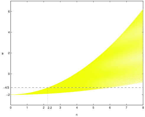
Figure 1: The restricted range of $\omega$ and $n$: The current observation restricts $\omega$ and $n$ in the shadow region, while the weak energy condition in 5-dimensional Brans-Dicke theory restricts $\omega\geq-\frac{4}{3}$.

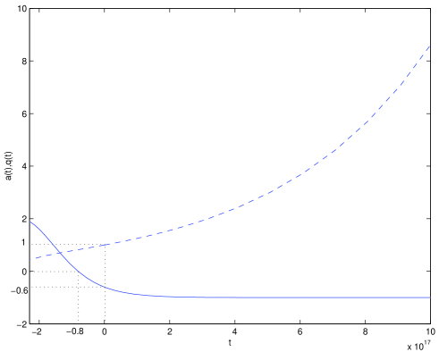
Figure 2: The evolution of $a(t)$ (dashed) and the deceleration parameter $q(t)$ (solid) are shown for the matter-dominated epoch with $\omega=-1.2$, $n=3$ and the current values: $\rho_{0}=3.8\times 10^{-28}kg\cdot m^{-3}$, $H_{0}=2.3\times 10^{-18}s^{-1}$, $a_{0}=\lambda_{0}=1$, and $\phi_{0}=1.5\times 10^{44}kg\cdot m^{-4}\cdot s^{2}$; here $t=0$ corresponds to today.

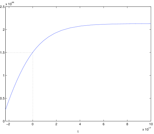
Figure 3: The evolution of $\phi(t)$ with the same parameters and current values as those in Fig.2, and $t=0$ corresponds to today.

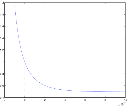
Figure 4: The evolution of $\lambda(t)$ with the same parameters and current values as those in Fig.2, and $t=0$ corresponds to today.

References

- [1] S. Perlmutter et. al., Astrophys. J. 483, 565(1997); Nature (London) 391, 51(1998); Astrophys. J. 517, 565(1999).
- [2] A. G. Riess et. al., Astrophys. J. 116, 1009(1998).
- [3] C. L. Bennett et. al., Astrophys. J. Suppl. 148, 1(2003).
- [4] P. J. E. Peebles and B. Ratra, Astrophys. J. Lett. 325, L17(1988).
- [5] A. Albrecht and C. Skordis, Phys. Rev. Lett. 84, 2076(2000).
- [6] I. Zlatev, L. Wang and P. J. Steinhardt, Phys. Rev. Lett. 82, 896(1999).
- [7] M. C. Bento, O. Bertolami, and N. C. Santos, Phys. Rev. D 65, 067301(2002).
- [8] D. Blais and D. Polarski, Phys. Rev. D 70, 084008(2004).
- [9] A. Y. Kamenshchik, U. Moschella, and V. Pasquier, Phys. Lett. B 511, 265(2001).
- [10] M. C. Bento, O. Bertolami, and A. A. Sen, Phys. Rev. D 66, 043507(2002).
- [11] C. Armendariz-Picon, V. Mukhanov, and P. J. Steinhardt, Phys. Rev. Lett. 85, 4438(2000).
- [12] R. J. Scherrer, Phys. Rev. Lett. 93, 011301(2004).
- [13] N. Banerjee and D. Pavon, Phys. Rev. D 63, 043504(2001).
- [14] S. Sen and A. A. Sen, Phys. Rev. D 63, 124006(2001).
- [15] C. Brans and R. H. Dicke, Phys. Rev. 124, 925(1961).
- [16] N. Mohammedi, Phys. Rev. D 65, 104018(2002).
- [17] F. Darabi, Class. Quantum. Grav. 20, 3385(2003).
- [18] T. Appelquist, A. Chodos, and P. G. O. Freund (ed.), Modern Kaluza-Klein Theories, Frontiers in Physics Series Vol.65(Addison-Wesley, Reading, MA, 1986).
- [19] M. Blagojevic, Gravitation and Gauge Symmetries, (IOP Publishing, 2002).
- [20] P. G. O. Freund, Nucl. Phys. B209, 146 (1982).
- [21] R. Geroch, J. Math. Phys. 12, 918(1971).
- [22] X. Yang, Y. Ma, J. Shao and W. Zhou, Phys. Rev. D 68, 024006(2003).
- [23] R. M. Wald, General Relativity, (University of Chicago Press: Chicago, 1984).
- [24] D. Spergel, et al., Astrophys. J. Suppl. 148, 175(2003).
- [25] S. G. Turyshev et. al., Lect. Notes Phys. 648, 301(2004).
- [26] W. L. Freedman and M. S. Turner, Rev. Mod. Phys. 75, 1433(2003).
- [27] L. Qiang and Y. Ma, in prepration.