1 Introduction

The quantum theory of gauge invariant cosmological perturbations is based on the validity of general relativity and quantum field theory. Both of these theories break down at Planckian scales. However if inflation lasts a little bit longer than what is required to solve the problems of standard cosmology- as predicted by most inflationary models [1]- many scales of cosmological size today have been sub-planckian at the onset of inflation. So it is natural to ask if the present cosmic microwave spectrum carries any thumbprint of physics at such small scales.

A number of papers have investigated the robustness of predictions of inflation to transplanckian physics by introducing non-linearities into the dispersion relation of Fourier modes [2, 3, 4, 5]. More general arguments [6], which may apply to any theory of quantum gravity [7], suggest a scenario in which the ultraviolet cutoff is modelled by a modified quantum mechanical commutation relation [8]:

$$[\mathbf{X},\mathbf{P}]=i\hbar(\mathbf{1}+\beta\mathbf{P}^{2})$$ (1)

This uncertainty relation has appeared in various studies of string theory [9]. Easther et.al. [10, 11] solved the equation for tensor perturbations numerically and found out that the effect on the tensor power spectrum is of order $\sigma=\sqrt{\beta}H$, where $\sqrt{\beta}$ is the minimal length associated with the hypothesized ultraviolet cutoff and $H$ is the Hubble constant during inflation.

However it was recently shown that this approach has an ambiguity: the presence of a cutoff not only affects the bulk terms of the Lagrangian density but also the boundary terms [12]. Hence a total time derivative added to the classical action will not remain a total time derivative in the presence of a cutoff. In general, it will lead to a modification of the equations of motion. In a recent paper we exploited the aforementioned modified commutation relation and the ambiguity associated with it to explain the origin of cosmic-scale primordial magnetic fields [13].

Vacuum fluctuations of the inflaton, $\phi_{0}$ – the field that drives inflation – produce both scalar and tensor perturbations, both of which contribute to the anisotropy of the cosmic microwave background radiation. For any inflationary model one can calculate $r$, the ratio of tensor to scalar amplitudes. $r$ multiplies the upper bound on the scalar density perturbations by a factor of $(1+r)^{-1/2}$. By knowing it one can tighten the bounds on the scalar spectral index [14, 15]. It is therefore important to know $r$ in as much detail as possible in order to extract cosmological parameters with more precision.

The effect of transplanckian physics on the tensor/scalar ratio was addressed for the first time in [16], where the authors discovered that the ratio will be influenced by the short distance physics, if tranplanckian physics does not lead to the same vacuum for scalar and tensor fluctuations. In this article, following the discovery of [12], we explore how the non-minimal choices of the boundary term for tensor and scalar fluctuations affect the tensor/scalar ratio. The structure of our paper is as follows: first, we present the equations that scalar and tensor fluctuations satisfy in the presence of a UV cutoff [12], categorizing various cases for which the ratio can change. Following ref. [10] we then solve these equations for scalar and tensor perturbations numerically in a near de-Sitter background. We compute how the scalar power spectrum varies as a function of $\sigma$. In the fourth section we ultimately find the ratio of tensor to scalar fluctuations.

2 Ratio of Tensor/Scalar Fluctuations with a Cutoff

Consider the action

$$S=\frac{1}{2}\int(\partial_{\mu}\phi\partial^{\mu}\phi-V(\phi))\sqrt{-g}~{}d^{4}x-\frac{1}{16\pi G}\int R\sqrt{-g}~{}d^{4}x$$ (2)

which describes a scalar inflaton field minimally coupled to gravity.  We assume that the metric $ds^{2}=a^{2}(\tau)\left({d\tau}^{2}-{\delta}_{ij}d{y}^{i}d{y}^{j}\right)$ describes the background, which is an homogenous isotropic Friedmann universe with zero spatial curvature.

We can decompose perturbations of the metric tensor into scalar, vector and tensor modes in the usual way according to their transformation properties under spatial coordinate transformations on the constant-time hypersurfaces. We shall be concerned with the scalar and tensor modes here, whose perturbative decomposition is given by

$$ds_{S}^{2} = a^{2}(\tau)\left((1+2\Phi)d\tau^{2}-2\partial_{i}Bdy^{i}d\tau-[(1-2\Psi)\delta_{ij}+2\partial_{i}\partial_{j}E]dy^{i}dy^{j}\right)$$ (3)

$$ds_{T}^{2} = a^{2}(\tau)\left(d\tau^{2}-[\delta_{ij}+h_{ij}]dx^{i}dx^{j}\right)$$ (4)

where $\Phi,B,\Psi$ and $E$ are scalar fields and $h_{ij}$ is a symmetric three-tensor field satisfying $h_{i}^{i}=0=h_{ij}{}^{,j}$. Fluctuations of the inflation field are given by $\phi(y,\tau)=\phi_{0}(\tau)+\delta\phi(y,\tau)$, where $\phi_{0}(\tau)$ is the homogenous part that drives the background expansion, with $|\delta\phi|\ll\phi_{0}$.

Using eqs. (3,4) and writing

$$\Re=-\frac{a^{\prime}}{a}\frac{\delta\phi}{\phi_{0}^{\prime}}-\Psi,$$ (5)

which is the gauge-invariant intrinsic curvature, the action can be written as [12]

$$S_{S}^{(1)}=\frac{1}{2}\int d\tau~{}d^{3}\mathbf{y}~{}z^{2}\left((\partial_{\tau}\Re)^{2}-\delta^{ij}~{}\partial_{i}\Re\partial_{j}\Re\right).$$ (6)

or alternatively as

$$S_{S}^{(2)}=\frac{1}{2}\int d\tau d^{3}\mathbf{y}\left({\left(\partial_{\tau}u\right)}^{2}-\delta^{ij}~{}{\partial}_{i}u~{}{\partial}_{j}u+\frac{z^{\prime\prime}}{z}u^{2}\right).$$ (7)

where $\Re=-u/z$ [17],

$$z=\frac{a\phi_{0}^{\prime}}{\alpha}$$ (8)

These two actions for scalar fluctuations are equivalent up to a boundary term in absence of minimal length, with $S_{S}^{(2)}$ more commonly used in the literature because of its similarity with the action of a massive free scalar field in Minkowskian space-time. However the effective mass, $z^{\prime\prime}/z$ is time dependent.

When the generalized uncertainty principal (1) is employed, $S_{S}^{(1)}$ and $S_{S}^{(2)}$ are no longer equivalent. Instead, they respectively yield the following equations of motion for the Fourier components of $u$, [12]:

$${u}_{\tilde{k}}^{\prime\prime}+\frac{{\kappa}^{\prime}}{{\kappa}}{u}_{\tilde{k}}^{\prime}+\left(\mu-\frac{z^{\prime\prime}}{z}-\frac{z^{\prime}}{z}\frac{{\kappa}^{\prime}}{{\kappa}}\right){u}_{\tilde{k}}=0,$$ (9)

$${u}_{\tilde{k}}^{\prime\prime}+\frac{{\kappa}^{\prime}}{{\kappa}}{u}_{\tilde{k}}^{\prime}+\left(\mu-\frac{z^{\prime\prime}}{z}\right){u}_{\tilde{k}}=0,$$ (10)

where

$$\mu(\tau,\rho) = \frac{a^{2}\rho^{2}}{(1-\beta\rho^{2})^{2}}$$ (11)

$$\kappa(\rho) = \frac{e^{3\beta\rho^{2}/2}}{1-\beta\rho^{2}}.$$ (12)

Here $\rho$ is a parameter that plays the role of inverse wavelength [18]. The difference in the above equations of motion is attributed to the non-triviality of the manner in which minimal length affects the boundary terms. The Scalar fluctuation amplitude is then defined as [19]

$$A_{S}(k)\equiv\frac{2}{5}P_{S}^{1/2}=\frac{2}{5}\sqrt{\frac{k^{3}}{2\pi^{2}}}\left|\frac{u_{\tilde{k}}}{z}\right|_{\tilde{k}/aH\rightarrow 0}.$$ (13)

Similarly, for tensor perturbations, among an infinite number of actions that are equivalent in the absence of minimal length we choose [12] to start from

$$S_{T}^{(1)}=\frac{m_{Pl}^{2}}{64\pi}\int d\tau d^{3}\mathbf{y}~{}a^{2}(\tau)~{}\partial_{\mu}h^{i}{}_{j}~{}\partial^{\mu}h_{i}{}^{j}$$ (14)

and

$$S_{T}^{(2)}=\frac{1}{2}\int d\tau d^{3}\mathbf{y}\left(\partial_{\tau}P_{i}{}^{j}\partial^{\tau}P^{i}{}_{j}-\delta^{rs}{\partial}_{r}P_{i}{}^{j}{\partial}_{s}P^{i}{}_{j}+\frac{a^{\prime\prime}}{a}P_{i}{}^{j}P^{i}{}_{j}\right),$$ (15)

that again differ from each other by a boundary term. As we will see, one of these actions has a minimal effect on tensor/scalar ratio whereas the other one has a maximal effect. Also, $S_{T}^{(1)}$ is the action one obtains by directly expanding the Einstein-Hilbert action. Here

$$P^{i}{}_{j}(y)=\sqrt{\frac{m_{Pl}^{2}}{32\pi}}~{}a(\tau)h^{i}{}_{j}(y)$$ (16)

and $h_{ij}$ is the transverse traceless part of tensor perturbations of the metric (4).

The $\tilde{k}$-Fourier component of $P_{ij}$ (denoted $p_{\tilde{k}}$), satisfies the following equation of motion using the cutoff modified $S_{T}^{(1)}$

$${p}_{\tilde{k}}^{\prime\prime}+\frac{{\kappa}^{\prime}}{{\kappa}}{p}_{\tilde{k}}^{\prime}+\left(\mu-\frac{a^{\prime\prime}}{a}-\frac{a^{\prime}}{a}\frac{{\kappa}^{\prime}}{{\kappa}}\right){p}_{\tilde{k}}=0,$$

whereas it satisfies

$${p}_{\tilde{k}}^{\prime\prime}+\frac{{\kappa}^{\prime}}{{\kappa}}{p}_{\tilde{k}}^{\prime}+\left(\mu-\frac{a^{\prime\prime}}{a}\right){p}_{\tilde{k}}=0.$$ (17)

if we employ the variational principal on the cutoff modified $S_{T}^{(2)}$.

We define the tensor amplitude as [19]

$$A_{T}(k)\equiv\frac{1}{10}P_{T}^{1/2}=\frac{1}{10}\sqrt{\frac{k^{3}}{2\pi^{2}}}\left|h_{\tilde{k}}\right|_{\tilde{k}/aH\rightarrow 0}$$ (18)

The ratio of tensor to scalar fluctuations and scalar spectral index are respectively given by

$$r\equiv\frac{A_{T}^{2}}{A_{S}^{2}},$$ (19)

$$n(k)-1\equiv\frac{d\ln A_{S}^{2}(k)}{d\ln k}.$$ (20)

The effect of $r$ is to multiply the upper bound on the density perturbations by a factor of $(1+r)^{-1/2}$ which in turn affects our estimation of the scalar spectral index [15, 14].

In the absence of minimal length, one can expand the ratio of tensor/scalar fluctuations in terms of the slow roll parameters. To first order it is [14, 19, 20]

$$\frac{A_{T}^{2}}{A_{S}^{2}}=\epsilon$$ (21)

where

$$\epsilon\equiv\frac{3\phi_{0}^{2}}{2}{\left(V(\phi_{0})+\frac{1}{2}{\dot{\phi}_{0}}^{2}\right)}^{-1}=\frac{m_{Pl}^{2}}{4\pi}\left(\frac{H_{\phi}}{H}\right)^{2}.$$ (22)

is the first slow-roll parameter [19]. Here, $\phi$ subscript denotes differentiation with respect to $\phi$. In the presence of minimal length the relation (21), takes the following form

$$\frac{A_{T}^{2}}{A_{S}^{2}}=\epsilon{\left|\frac{p_{k}}{u_{k}}\right|}_{k/aH\rightarrow 0}^{2}$$ (23)

The ambiguity in choosing the actions for scalar and tensor fluctuations in the presence of the minimum length is a new source of transplanckian effects that can modify the tensor/scalar ratio $r$. In general we have four possibilities:

I,II

If we choose either $(S_{S}^{(1)},S_{T}^{(1)})$ or $(S_{S}^{(2)},S_{T}^{(2)})$ as the actions describing scalar and tensor fluctuations, the scalar modes $u_{\tilde{k}}$, and tensor modes $p_{\tilde{k}}$, satisfy differential equations that are as similar as possible. In particular this implies that in the special cases of near-de-Sitter and power-law inflation where $z^{\prime\prime}/z=a^{\prime\prime}/a$ (see [19]) and $z^{\prime}/z=a^{\prime}/a$ (see Appendix), the equations governing both scalar and tensor perturbations are identical. Since metric and inflaton perturbations cannot be fully distinguished in a gauge invariant manner, scalar and tensor modes should also obey the same initial conditions, yielding $\left|\frac{p_{k}}{u_{k}}\right|=1$. The distinction between cases I and II becomes apparent when the inflating background deviates from the power-law and near-de-sitter backgrounds.

III,IV

The other extreme is to select either of the pairs $(S_{S}^{(1)},S_{T}^{(2)})$ or $(S_{S}^{(2)},S_{T}^{(1)})$ to describe the situation. In these cases the modes $u_{\tilde{k}}$ and $p_{\tilde{k}}$, satisfy differential equations of differing form even in near-de-Sitter and power-law backgrounds. In particular the tensor amplitude is not just $\epsilon$ times the scalar amplitude in power-law backgrounds. In the next section we present a complete analysis of the scalar and tensor spectra in near-de-Sitter space. We will investigate how the ratio of tensor to scalar perturbations varies as a function of $\sigma$, the ratio of minimal length to Hubble length during inflation.

3 Scalar perturbations with minimum length in near-de-Sitter space

Curvature fluctuations arise because the value of the inflaton field is coupled to the energy density of the vacuum energy driving inflation, i.e. fluctuations in the inflaton field result in fluctuations in the expansion rate at linear order in perturbation theory. This coupling is what creates fluctuations in the intrinsic curvature scalar, which are then manifest as density fluctuations. Since in de Sitter space fluctuations in the inflaton field, $\phi$, are not coupled to fluctuations in the energy density, the amplitude of density fluctuations is zero. A naive exploitation of the formalism of refs. [17, 19] implies that the expression for density fluctuations is singular for de Sitter space. The reason that the expression is singular is not because the density fluctuation amplitude is singular, but because the foliation of space-time implicit in the choice of gauge becomes singular.

Nevertheless, we can proceed in this manner by assuming that $\epsilon$ is close to zero, i.e. that the background is arbitrarily close to the de Sitter limit. Note that we are taking $H$, the Hubble parameter, to be very small, since it is known from COBE that $P_{S}=H^{2}/\epsilon\simeq const.\times 10^{-5}$.

We begin with an analysis of the scalar power spectrum, tracking the normalized modes which are inside the horizon until they are far outside the horizon, where their amplitude determines the perturbation spectrum. To this end, we will solve the mode equation (9) numerically. As in Ref.[10, 11], we describe the initial evolution by an approximate analytic solution, which we then evolve numerically to late times.

In this section and in what follows, we first analyze the action $S_{S}^{(2)}$ and $S_{T}^{(1)}$ for scalar and tensor perturbations respectively. In de Sitter space $a=-1/(H\tau)$ and $z^{\prime\prime}/z=2/\tau^{2}$. A mode with a fixed comoving wave number $\tilde{k}$ corresponds over time to increasing proper wave lengths. Each mode’s proper wave length corresponds to the Planck length at some time $\tau$ that depends on $\tilde{k}$ and this is when the evolution of that mode begins. This time is when $a^{2}(\tau_{\tilde{k}})\simeq\beta\tilde{k}^{2}$ and $\rho^{2}=1/\beta$. At this initial time equation (9) has an irregular singular point.

Since de Sitter space is time-translation invariant, the equation can be written in terms of the dimensionless parameter $w=\tilde{k}\tau$, in terms of which all the modes evolve jointly:

$$\frac{d^{2}u_{\tilde{k}}}{dw^{2}}+n(w)\frac{du_{\tilde{k}}}{dw}+\Omega^{2}(w)u_{\tilde{k}}(w)=0,$$ (24)

where

$$n(w) = \frac{1}{\theta(\zeta(w))}\frac{d\theta(\zeta(w))}{dw}$$ (25)

$$\Omega^{2}(w) = -\left(\frac{1}{\sigma^{2}w^{2}}\frac{W(\zeta(w))}{(1+W(\zeta(w)))^{2}}+\frac{2}{w^{2}}\right)$$ (26)

and in de Sitter space $\zeta(w)=-\sigma^{2}w^{2}$. Here we define

$$\sigma=\sqrt{\beta}/H^{-1},$$ (27)

which is the ratio of the minimal length scale and the Hubble length scale during inflation. The function $W(x)$ is the Lambert W-function, defined by the relation $W(x)e^{W(x)}=x$ [21].

Equation (24) has a singular point at $w_{crit}=\varpi=-\frac{1}{\sigma\sqrt{e}}$. The singular point at $\varpi$ is an irregular singular point because the coefficients of $du_{\tilde{k}}/dw$ and $u_{\tilde{k}}$ are not analytic in $v=w-\varpi$

$$n(v) = -\frac{1}{2v}-\frac{7}{12}\frac{e^{1/2}}{\sqrt{Av}}+\frac{67}{144}\frac{e}{A}+\cdots$$

$$\Omega^{2}(v) = \frac{A}{v}-\frac{e^{1/2}\sqrt{A}}{\sqrt{v}}-\frac{37}{72}e+\cdots$$ (28)

where

$$A=\frac{e^{1/2}}{4\sigma}.$$ (29)

Proceeding along the lines given in ref. [10, 11], we solve for the leading behavior of $u_{\tilde{k}}$ by extracting the most singular terms of the equation of motion

$$\ddot{u}_{\tilde{k}}-\frac{1}{2v}\dot{u}_{\tilde{k}}+\frac{A}{v}u_{\tilde{k}}=0.$$ (30)

where in the overdot now denotes the derivative with respect to $v$. Ignoring the $\dot{u}_{\tilde{k}}$ term, this equation is similar to the high frequency limit of the mode equation:

$$u_{k}^{\prime\prime}(\tau)+\Omega_{k}^{2}(\tau)u_{k}(\tau)=0$$ (31)

whose solution is approximated by the WKB form

$$u_{k}(\tau)=\frac{1}{\sqrt{2\Omega_{k}}}\exp(-i\int^{\tau}\Omega_{k}(\tau^{\prime})d\tau^{\prime})$$ (32)

if the adiabatic condition $|\Omega_{k}^{\prime}/\Omega_{k}^{2}|\ll 1$ is satisfied. This choice of vacuum, which is called Bunch-Davies vacuum, reduces to the Minkowskian vacuum for wavelengths smaller than the Hubble scale. Inspired by this similarity, one can suggest a Bunch-Davies-like vacuum of the form:

$$u_{\tilde{k}}(v)=(\frac{v}{4{\tilde{k}}^{2}A})^{1/4}\exp(-2i\sqrt{Av})$$ (33)

with

$$\Omega_{\tilde{k}}=\tilde{k}\sqrt{A/v}.$$ (34)

This vacuum does not satisfy the adiabaticity conditions in the vicinity of its creation time, $v=0$. To be specific:

$$\frac{\Omega_{\tilde{k}}^{\prime}}{\Omega_{\tilde{k}}^{2}}=\frac{\tilde{k}}{2}\frac{1}{\sqrt{Av}}$$ (35)

For $v\sim 0$ the adiabatic condition is violated. It means that each mode is born in an excited state. In the model of transplanckian physics proposed in ref.[2], each mode undergoes three phases in its evolution. In the first phase, the wavelength of the given mode is much smaller than the Planck length: $\lambda\ll l_{p}$. Each mode is born into the vacuum state that minimizes the Hamiltonian and satisfies the adiabaticity condition. In the second phase, the wavelength of the mode is larger than the Planck length but still smaller than the Hubble radius, $l_{p}\ll\lambda\ll l_{H}$. In the third phase the mode is outside the Hubble radius: $\lambda\gg l_{H}$. In our version of this scenario, the first phase is removed and replaced by an excited initial state which violates the adiabaticity conditions.

In fact, equation (30) is solved exactly by

$$u(y)=C_{+}F(v)+C_{-}F^{\ast}(v)$$ (36)

where

$$F(y)=(\frac{\sqrt{A}}{2}+iA\sqrt{v})\exp(-2i\sqrt{Av})$$ (37)

and where the coefficients $C_{\pm}$ are constrained through the Wronskian condition:

$$u_{\tilde{k}}(\tau)u_{\tilde{k}}^{\ast^{\prime}}(\tau)-u_{\tilde{k}}^{\ast}(\tau)u_{\tilde{k}}^{\prime}(\tau)=i{\kappa}^{-1},$$ (38)

that reduces to

$$|C_{+}|^{2}-|C_{-}|^{2}=\frac{e^{-1}}{2\tilde{k}A^{3}}.$$ (39)

This equation will lead to a one parameter family of solutions. Similarity with the Bunch-Davies vacuum suggests that $C_{-}=0$. In addition, in this case, it is possible to obtain conventional QFT result when $\sigma\rightarrow 0$. However there exist other legitimate choices of the vacuum. Specifically, it is possible to recover the standard QFT result in the limit $\sigma\rightarrow 0$, if $C_{-}$ approaches zero faster than $\sigma^{3/2}$, as we shall subsequently demonstrate. However we will first assume that $C_{-}=0$.

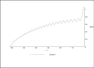
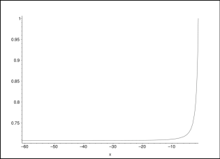
Figure 1: The left figure shows how each mode evolves in the presence of a cutoff as a function of $w=\tilde{k}\tau$. Each mode is created at a finite conformal time and the amplitude of the modes is modulated on a monotonously increasing curve. $C_{-}$ is assumed to be zero. The right figure shows how in absence of minimal length each mode is created at infinite conformal time and its amplitude monotonously increases until it leaves the horizon.

Equation (24) has been solved to order $1/v$. As in Ref.[10] we will extract the subleading behavior of $u_{\tilde{k}}$ by the method of dominant balance [22]. We solve the differential equation (24) up to $1/\sqrt{v}$ by defining $u_{\tilde{k}}(v)=F(v)(1+\epsilon_{1}(v))$, extracting the most singular terms. The equation of motion for $\epsilon_{1}$ is:

$$\frac{d^{2}\epsilon_{1}}{dv^{2}}-\frac{1}{2v}\frac{d\epsilon_{1}}{dv}-\frac{3}{2}e^{1/2}\sqrt{\frac{A}{v}}=0$$ (40)

which has the solution

$$\epsilon_{1}(v)=\frac{1}{3}\sqrt{A}e^{1/2}v^{3/2}(3\ln(v)-2).$$ (41)

The solution is improved by extracting the residual $\ln(v)$ terms. To do so, we replace $u_{\tilde{k}}$ by $F(v)(1+\epsilon_{1}(v))(1+\epsilon_{2}(v))$ and extract the most singular terms to obtain the following differential equation for $\epsilon_{2}(v)$

$$\frac{d^{2}\epsilon_{2}}{dv^{2}}-\frac{1}{2v}\frac{d\epsilon_{2}}{dv}-\frac{7}{8}e\ln(v)=0.$$ (42)

whose solution is

$$\epsilon_{2}(v)=\frac{7}{16}ev^{2}(2\ln(v)-5).$$ (43)

We have solved the differential equation (24) up to terms that vanish as $v\rightarrow 0$. We glue this analytic solution, which is valid when the mode is in the vicinity of the irregular singular point and inside the horizon, to the full numerical evaluation of the mode equation. As the coefficients of $u_{\tilde{k}}$ and $u_{\tilde{k}}^{\prime}$ are infinite at $v=0$, this junction is done at a finite nonzero value of $v_{0}$. By varying $v_{0}$ we have checked that our results do not depend on the choice of starting point. We evolved the mode equation using Fehlberg fourth-fifth order Runge-Kutta method implemented in Maple $9$. In Figure (1) we have shown how each fluctuation mode evolves as a function of $w=\tilde{k}\tau$. In the absence of minimal length there is no birth time for the modes and $|u_{k}|$ increases monotonically as it evolves. As we incorporate minimal length into the problem, each mode is created at a definite $\tilde{k}$-dependent time and $|u_{\tilde{k}}|$ is modulated on a monotonically increasing function until it crosses the horizon. At that time $|u_{k}|$ stops oscillating and goes to infinity as we approach the present time. One should notice that parameter $\tilde{k}$ is different from the comoving momentum at large momenta. This difference modifies the condition of horizon crossing in terms of the parameter $\tilde{k}$. Note that $\rho$ plays the role of inverse wavelength in our model [18]. Using the relation between $\rho$ and $\tilde{k}$ [12],

$$\tilde{k}^{i}=a\rho^{i}e^{-\beta\rho^{2}/2},$$ (44)

we can express the criterion of horizon crossing , $\rho=H$, in terms of parameter $\tilde{k}$

Figure 2: The dependence of $\frac{\sqrt{2}{\pi}\dot{\phi}}{H^{2}}P_{S}^{1/2}$ is plotted against $\sigma$. As $\sigma$ goes to zero, the standard result of $\frac{1}{\sqrt{2}}$ is obtained. It is assumed that $C_{-}=0$.

$$\tilde{k}=aH\exp(-\beta H^{2}/2)$$ (45)

which takes the following form in de Sitter space

$$w_{\text{horizon}}=-\exp(-\sigma^{2}/2)$$ (46)

where $w=\tilde{k}\tau$. In absence of minimal length this criterion reduces to the familiar one in de Sitter space, $w=-1$.

Figure 3: The left figure shows the dependence of $\frac{\sqrt{2}{\pi}\dot{\phi}}{H^{2}}P_{S}^{1/2}$ against $\sigma$ when $C_{-}/C_{+}=0.5$. The right figure graphs the dependence of $\frac{\sqrt{2}{\pi}\dot{\phi}}{H^{2}}P_{S}^{1/2}$ on $\sigma$ when $C_{-}\propto\sigma$. In neither of these cases do we recover the standard field theory result when $\sigma\rightarrow 0$.

For values of $\sigma$ close to $1$, i.e. when the energy scale of inflation is of the order of the minimal length, the horizon-crossing condition is considerably modified. Of course, we are really interested in the asymptotic values of $|u_{\tilde{k}}|$, when $\rho/H\rightarrow 0$. To implement it numerically, we have assumed this condition is satisfied when $\rho/H=0.01$. We can express this condition in terms of parameter $w$:

$$w_{\text{asymp}}=-0.01\exp(-\sigma^{2}/20000).$$ (47)

The general answer to Equation(24), has the form of $u_{\tilde{k}}(\tau)=N(\tilde{k})U_{\tilde{k}}(w)$. Comparison with Equation (39) yields $N(\tilde{k})=1/\sqrt{\tilde{k}}$. So, the power spectrum in near-de Sitter space is:

$$P_{S}^{1/2}=\sqrt{\frac{\tilde{k}^{3}}{2\pi^{2}}}\left|\frac{u_{\tilde{k}}}{z}\right|=\frac{H^{2}}{\dot{\phi}}\frac{\left|-wU_{\tilde{k}}(w)\right|}{\pi\sqrt{2}}|_{w=w_{\text{asymp}}}$$ (48)

On the other hand, quantum field theory yields the following result for the near-de Sitter space

$$P_{S}^{1/2}(\sigma=0)=\frac{H^{2}}{2\pi\dot{\phi}}$$ (49)

Figure 4: The left figure shows the dependence of $\frac{\sqrt{2}{\pi}}{H}P_{S}^{1/2}$ against $\sigma$ when $C_{-}\propto\sigma^{2}$. The right figure shows the ratio of scalar power spectrum when $C_{-}=0$ to scalar power spectrum when $C_{-}\propto\sigma^{2}$. In this case the scalar power spectrum approaches the standard result when $\sigma\rightarrow 0$

In Fig.$2$ we have displayed the $\sigma$ dependence of the scalar power spectrum when $C_{-}=0$. For small values of $\sigma$, the power spectrum has an oscillatory behavior around its standard result. For sufficiently large values of $\sigma$ the power spectrum is significantly suppressed. This could be used as a mechanism for solving the fine tuning problem of inflationary models [10].

Next we relax the condition $C_{-}=0$. Equation (39) will lead to a one parameter family of solutions. The criterion of approaching the result of conventional quantum field theory when $\sigma\rightarrow 0$ can be used to constrain our space of solutions. It has been pointed out [10] that if the ratio of $C_{-}/C_{+}$ is a non-zero constant then the tensor power spectrum does not approach its standard result in the limit $\sigma\rightarrow 0$ . In Fig.3, we have examined this statement for scalar perturbations and noticed that the same thing happens for scalar perturbations too. However, in general, $C_{-}$ can be a function of $\sigma$. Since we know that when $C_{-}=0$ and $C_{+}\propto\sigma^{3/2}$, we obtain the standard result in the limit of $\sigma\rightarrow 0$, we expect that if $C_{-}$ approaches zero faster than $\sigma^{3/2}$ when $\sigma\rightarrow 0$ the criterion of recovering the standard QFT result is satisfied. We have verified this statement for $C_{-}\propto\sigma$ and $C_{-}\propto\sigma^{2}$ respectively as shown in Figures 3 and 4. Hence we conjecture that it is possible that $C_{-}$ be proportional to $\sigma^{n}$, $n>\frac{3}{2}$ whilst obtaining the standard QFT result in the limit $\sigma\rightarrow 0$.

In most inflationary models the expansion rate is slower than de Sitter space; the ratio of minimum length to physical horizon is not constant and decreases towards the end of inflation. Our study of de Sitter space suggests that the amplitude of the longer modes will be affected more. Whether it has observable effects depends on the energy scale of inflation. We plan to return to this problem in future work [23].

4 Ratio of tensor to scalar perturbations with minimum length in near-de Sitter space

As explained above, if the action of the tensor perturbations, in absence of $\sigma$, is given in eq.(15) then the tensor power spectrum will be $\epsilon$ times that of the scalar perturbations. Otherwise, if the action is given by eq. (14), its power spectrum will not be a simple multiple of the scalar perturbations. Although a complete analysis of the equation of motion derived from this action has been done once in de Sitter space [10], we recapitulate those calculations in the present context to find the ratio of tensor to scalar fluctuations. The outline of the calculations is completely similar to what was done for scalar perturbations: we tailor the solution that is valid in vicinity of the irregular singular point to the numerically integrated solution. The exact analytic solution in the neighborhood of the singular point is:

Figure 5: The dependence of $\frac{\sqrt{\pi}m_{P}}{4H}P_{T}^{1/2}$ is plotted against $\frac{\sqrt{\pi}m_{P}}{4H}P_{T}^{1/2}$ approaches the standard result of $\frac{1}{\sqrt{2}}$ as $\sigma$ goes to zero. We have assumed that $D_{-}=0$.

$$u_{\tilde{k}}=D_{+}G(v)(1+\xi_{1}(v))(1+\xi_{2}(v))+D_{-}G^{\ast}(v)(1+\xi_{1}(v))(1+\xi_{2}(v))$$ (50)

where

$$G(y) = (\frac{\sqrt{B}}{2}+iB\sqrt{v})\exp(-2i\sqrt{Bv}),$$

$$\xi_{1}(v) = \frac{1}{3}e^{1/2}v^{3/2}\sqrt{A}(3\ln(v)-2),$$

$$\xi_{2}(v) = \frac{7}{8}ev^{2}\ln(v)-\frac{35}{16}ev^{2},$$ (51)

$$B=\frac{1}{8}\frac{8A^{2}+e}{A}$$ (52)

$D_{+}$ and $D_{-}$ are constrained by the following wronskian condition

$$|D_{+}|^{2}-|D_{-}|^{2}=\frac{e^{-1}}{2\tilde{k}B^{3}}$$ (53)

Again, we have considerable freedom in choosing our vacuum. Since the right-hand side of eq.(89) approaches zero like $\sigma^{3}$ when $\sigma\rightarrow 0$, if $D_{-}$ tends to zero faster than $\sigma^{3/2}$ we can recover the standard QFT result. Hereafter we restrict ourselves to $D_{-}=0$ so as to have a Bunch-Davies-like vacuum. We use equation (53) with $D_{-}=0$ at a point close to the singularity to integrate the differential equation. In Fig.5 we have displayed the $\sigma$-dependence of the tensor power spectrum. The oscillationary behavior in vicinity of $\sigma=0$ and decaying behavior for larger values of $\sigma$ has repeated.

Figure 6: The dependence of $\frac{P_{T}^{1/2}}{4\sqrt{\epsilon}P_{S}^{1/2}}$ is plotted against $\sigma$. It approaches the standard result of unity as $\sigma$ goes to zero. $C_{-}$ and $D_{-}$ are set to zero.

Fig.6 shows how the tensor to scalar perturbations ratio varies as a function of $\sigma$ when $C_{-}=D_{-}=0$. For small values of $\sigma$, it oscillates about its standard value, $\epsilon$. For intermediate values of $\sigma$ it remains almost constant on a value that is less than its standard result. Although the tensor and scalar fluctuations both decrease as $\sigma$ increases, their ratio gradually increases by increasing $\sigma$ and even becomes larger than its standard value. This means that the tensor fluctuations decrease more slowly than do the scalar fluctuations.

We can derive some qualitative features of the same study for power-law backgrounds from what we derived in near-de Sitter space. At the beginning of inflation the expansion is faster than it is at the end of inflation and so the Hubble parameter is larger. Hence the effect is much more profound for modes that leave the horizon at that time. For such modes, the ratio will be much more distorted from standard predictions. We plan to return to this problem in greater detail [23].

Now we assume that $S_{S}^{(1)}$ and $S_{T}^{(2)}$ describes the behavior of scalar and tensor perturbation. In near-De-sitter and power-law backgrounds the equation derived from $S_{S}^{(1)}$ and $S_{T}^{(2)}$ are the same as the ones derived from $S_{T}^{(1)}$ and $S_{S}^{(2)}$ respectively. Therefore the ratio $\frac{A_{T}^{2}}{\epsilon A_{S}^{2}}$ will be reversed. Fig.7 shows that how the ratio of tensor to scalar perturbations varies as a function of $\sigma$. The same oscilationary behavior in vicinity of $\sigma=0$ has repeated. However in this case the tensor/scalar ratio decreases as the ratio of minimal length approaches the Hubble length during the inflation. This mechanism might be used to dampen the contribution of tensor amplitudes to the anisotropy of the microwave background radiation.

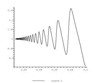
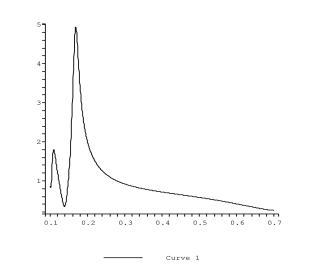
Figure 7: The dependence of $\frac{P_{T}^{1/2}}{4\sqrt{\epsilon}P_{S}^{1/2}}$ is plotted against $\sigma$. It approaches the standard result of unity as $\sigma$ goes to zero. $C_{-}$ and $D_{-}$ are set to zero. It is assumed that $S_{S}^{(1)}$ and $S_{T}^{(2)}$ describes the behavior of scalar and tensor perturbation, respectively.

5 Conclusion

Both tensor and scalar perturbations are responsible for the anisotropy of the CMB. Knowledge of the ratio of tensor/scalar perturbations provides an important constraint on related cosmological parameters.

We have investigated the implications of implementing a minimal length hypothesis from the generalized uncertainty principle (1) for the tensor/scalar ratio $r$ in inflationary scenarios. Specifically, we have studied how an ambiguity generically present in this hypothesis [12] leads to different conclusions about how and whether transplanckian physics alters $r$. In two of the cases the ratio remains constant, unless the background deviates from a power-law expansion during inflation. In the other two cases, the ratio is modified even in a simple de Sitter or power-law background. We also found the dependence of the ratio on the minimal length for the near-de-Sitter background in these two cases.

The tensor fluctuations are expected to contribute to the CMB’s $B$ -polarization. This effect may be observable with the upcoming PLANCK satellite. One can then differentiate the contribution of tensor fluctuations from scalar ones to check the above scenario.

Appendix

The scalar gauge invariant parameter, $u$, is proportional to $\Re$, the intrinsic curvature perturbations of the spatial hypersurface through a factor $z$ (8) which equivalently can be defined as:

$$z=\frac{a\dot{\phi_{0}}}{H}$$ (54)

where $H$ is the Hubble parameter, $\dot{a}/a$ (dot denotes differentiation with respect to the physical time). So one obtains:

$$\frac{z^{\prime}}{z}=\frac{a^{\prime}}{a}+\frac{\dot{\phi_{0}}^{\prime}}{\dot{\phi_{0}}}-\frac{H^{\prime}}{H}.$$ (55)

$\dot{\phi_{0}}^{\prime}/\dot{\phi_{0}}$ can be written as $a\ddot{\phi_{0}}/\dot{\phi_{0}}$. Using the definition of $\eta$

$$\eta(\phi)\equiv-\frac{\ddot{\phi_{0}}}{H\dot{\phi_{0}}}=\frac{m_{Pl}^{2}}{4\pi}\left(\frac{H_{\phi\phi}}{H}\right)=\epsilon-\frac{m_{Pl}{\epsilon}_{\phi}}{\sqrt{16\pi\epsilon}},$$ (56)

this can be written in terms of the slow roll parameters:

$$\frac{\dot{\phi_{0}}^{\prime}}{\dot{\phi_{0}}}=-\eta\frac{a^{\prime}}{a}.$$ (57)

$H^{\prime}/H$ is equal to $a\dot{\phi_{0}}H_{\phi}/H$. Choosing the convention that $\dot{\phi_{0}}>0$, from Eq. (22) one derives:

$$\frac{H_{\phi}}{H}=-\frac{2\sqrt{\pi\epsilon}}{m_{Pl}}$$ (58)

and

$$\dot{\phi_{0}}^{2}=\frac{2\epsilon V}{3-\epsilon}.$$ (59)

The inflaton energy density is $\frac{\dot{\phi_{0}}^{2}}{2}+V$ and the first Friedmann equation

$$H^{2}=\frac{8\pi}{3m_{Pl}^{2}}(\frac{\dot{\phi_{0}}^{2}}{2}+V),$$ (60)

combined with (59), yields:

$$V=\frac{m_{Pl}^{2}H^{2}(3-\epsilon)}{8\pi}.$$ (61)

From Equations (59)and (61) one concludes:

$$\dot{\phi_{0}}=\frac{m_{Pl}H}{2}\sqrt{\frac{\epsilon}{\pi}}.$$ (62)

Using the above equation one obtains:

$$\frac{H^{\prime}}{H}=-\epsilon\frac{a^{\prime}}{a}.$$ (63)

Inserting equations (63) & (57) back into eq.(55), we obtain the following expansion for $z^{\prime}/z$ in terms of the slow roll parameters:

$$\frac{z^{\prime}}{z}=\frac{a^{\prime}}{a}(1+\epsilon-\eta).$$ (64)

In power-law and near-De-sitter space $\epsilon=\eta$ and so $z^{\prime}/z=a^{\prime}/a$.

References

- [1] A. D. Linde, Particle Physics and Inflationary Cosmology (Harwood Academic, Chur, Switzerland).
- [2] J. Martin & R. H. Brandenberger, Phys. Rev. D63, 123501 (2001), hep-th/0005209.
- [3] J. C. Niemeyer, Phys. Rev. D63, 123502 (2001), astro-ph/0005533.
- [4] J. Kowalski-Glikman, Phys. Lett. B499,1 (2001), astro-ph/0006250.
- [5] J. C. Niemeyer & R. Parentani Phys. Rev. D64 101301 (2001), astro-ph/0101451.
- [6] A. Kempf, hep-th/9810215.
- [7] A. Kempf, Phys. Rev. D63, 083514 (2001), astro-ph/0009209.
- [8] A. Kempf, G. Mangano and R.B. Mann, Phys. Rev. D52, 1108 (1995).
- [9] G. Veneziano, Europhys. Lett. 2 199 (1986); D. Gross & P. Mende, Nucl. Phys. B303 407 (1988); D. Amati, M. Ciafaloni & G. Veneziano, Phys. Lett. B216 41 (1989).
- [10] R. Easther, B. Greene, W. H. Kinney, G. Shiu, Phys. Rev. D64 103502 (2001), hep-th/0104102.
- [11] R. Easther, B. Greene, W. H. Kinney, G. Shiu, Phys. Rev. D67 063508 (2003), hep-th/0110226.
- [12] A. Ashoorioon, A. Kempf, R. B. Mann, Phys. Rev. D71 023503 (2005), astro-ph/0410139.
- [13] A. Ashoorioon, R. B. Mann, Phys. Rev. D71 103509 (2005), gr-qc/0410053.
- [14] A. R. Liddle, D. H. Lyth, Phys. Lett. B291 391 (1992).
- [15] D. S. Salopek, Phys. Rev. Lett. 69 3602 (1992).
- [16] L. Hui & W. H. Kinney, Phys.Rev. D65 103507 (2002).
- [17] V. F. Mukhanov, JETP 41, 493 (1985), V. F. Mukhanov, Zh. Eksp. Teor. Fiz. 94, 1 [Sov. Phys. JETP Lett. 41, 493 (1988)], V. F. Mukhanov, H. A. Feldman, R. H. Brandenberger, Phys. Rep. 215, 203 (1992).
- [18] A. Kempf, private communications.
- [19] J. E. Lidsey, A. R. Liddle, E. W. Kolb, E. J. Copeland, T. Barreiro & M. Abney, Rev. Mod. Phys. 69, 373 (1997).
- [20] D. Stewart, D. H. Lyth, Phys. Lett 302B, 171 (1993).
- [21] R. Corless, G. Gonnet, D. Hare, D. Jeffrey, and D. Knuth, Adv. Comput. Math. 5, 329 (1996).
- [22] Carl M. Bender and Steven A. Orszag, ”Advanced Mathematical Methods for Scientists and Engineers”, McGrawHill, Inc., 1978.
- [23] A. Ashoorioon, J. Hovdebo, R. B. Mann, gr-qc/0504135.