Observation results by the TAMA300 detector
on gravitational wave bursts from stellar-core collapses

Abstract

We present data-analysis schemes and results of observations with the TAMA300 gravitational-wave detector, targeting burst signals from stellar-core collapse events. In analyses for burst gravitational waves, the detection and fake-reduction schemes are different from well-investigated ones for a chirp-wave analysis, because precise waveform templates are not available. We used an excess-power filter for the extraction of gravitational-wave candidates, and developed two methods for the reduction of fake events caused by non-stationary noises of the detector. These analysis schemes were applied to real data from the TAMA300 interferometric gravitational wave detector. As a result, fake events were reduced by a factor of about 1000 in the best cases. The resultant event candidates were interpreted from an astronomical viewpoint. We set an upper limit of $2.2\times 10^{3}$ events/sec on the burst gravitational-wave event rate in our Galaxy with a confidence level of 90%. This work sets a milestone and prospects on the search for burst gravitational waves, by establishing an analysis scheme for the observation data from an interferometric gravitational wave detector.

I Introduction

Direct observations of gravitational waves (GWs) will reveal new aspects of the universe bun-thorne1 . Since GWs are emitted by the bulk motion of matter, and are hardly absorbed or scattered, they have a potential to carry astrophysical and cosmological information different from that by electromagnetic waves. In order to create a new field of GW astronomy, several groups around the world are developing and operating GW detectors. Among them, much effort is being made recently on interferometric detectors: LIGO bun-LIGO in U.S.A., VIRGO bun-VIRGO and GEO bun-GEO in Europe, and TAMA bun-TAMA1 ; bun-TAMA3 in Japan. These detectors have wide-frequency-band sensitivity between about 10 Hz and a few kHz range, and have an ability to observe the waveform of a GW, which would contain astrophysical information. In these detectors, both high sensitivity and high stability are required because GW signals are expected to be extremely faint and rare.

There are several kinds of target GW sources in these interferometric detectors bun-thorne2 ; bun-schutz , and data-analysis schemes are being developed and applied to the observation data. Since GW signals are considered to be faint, an efficient data-analysis scheme is required to extract the remains of GWs from noisy detector outputs. The target GWs are classified by the signal waveforms: chirp waves, continuous waves, burst waves, and so on. A chirp wave is a sinusoidal waveform with increasing frequency and amplitude in time, which is radiated from an inspiraling compact binary just before its merger. Since this waveform is well-predicted, an effective and sophisticated method of matched filtering is used in chirp-wave search; correlations between the data and a template (the predicted waveform) are calculated to extract a GW signal from noisy data bun-BA ; bun-Tagoshi . A continuous wave has a sinusoidal waveform with a stable frequency for over many years, which is radiated from a quasi-stationary compact binary or a rotating neutron star. A matched filtering method can also be used in the search for continuous waves from known sources, because we can predict their waveforms precisely by observations with electromagnetic waves bun-Niebauer ; bun-LIGOcont .

A burst wave, which is the target of this article, is also a promising gravitational-waveform class. This wave has a short spike-like waveform with a duration time of less than 100 msec, which is emitted from stellar-core collapse in a supernova explosion or a merger of a binary system. Unlike the chirp and continuous-wave cases, a matched filtering method cannot be used in a burst-wave analysis. This is because a set of precise waveform templates that cover the source parameters is not available, while typical waveforms are obtained by numerical simulations bun-SNwave0 ; bun-SNwave1 ; bun-SNwave2 . Thus, several signal-extraction methods, called ’burst filters’, have been proposed for the detection of these burst gravitational waves: an excess power filter bun-excesspow , a cluster filter in the time-frequency plane bun-TFcluster , a slope (or a linear-fit) filter bun-slope , and a pulse correlation filter bun-cor . Since we have only a little knowledge on the waveforms, these filters look for unusual events in the Gaussian-noise background.

For the detection of GWs, evaluation and reduction of fake-event backgrounds are critical problems. In each analysis scheme described above, we define an evaluation filter (such as a correlation with the template in a matched filtering method, and certain statistics describing any unusual behavior of the data in burst analyses), and record the filter output as a GW event trigger if it is above a given threshold. The event triggers usually contain fake events, which are caused by statistical and externally induced excesses in the detector noise level. Although an ideal interferometric detector would have a stationary Gaussian-noise behavior, the detector output is far from stationary in practice, affected by external disturbances, such as seismic motion, acoustic disturbance, changes in the temperature and pressure and so on. As a result, it is likely that real signals are buried in these fake events, or are dismissed with a larger detection threshold set to reduce fakes. Thus, rejection of these fake events, or a veto in other words, is indispensable for the detection of GWs. In a chirp-wave analysis case, the output of the matched filter is less affected by non-stationary noises because it is only sensitive to a waveform similar to GWs. In addition, since we know a precise waveform of the target GW signal, we can reject the fake events by evaluating how well the candidate waveform fits to the template bun-BA ; bun-Tagoshi ; bun-BAveto . On the other hand, the affects of fake events are more serious and critical in the burst analysis case. Since burst filters are designed to extract any unusual behavior of the detector output, they are also sensitive to non-stationary noises by their nature. Moreover, it is not straightforward to distinguish these fakes from a real signal, and to reject them, because we do not know the precise GW waveforms.

There are several schemes to reject these fake events: coincidences by multiple detectors, veto analyses with detector monitor signals, rejection by waveform behaviors, and so on. Among them, the most powerful and reliable way will be a coincidence analysis with multiple independent detectors bun-coin1 ; bun-coin2 ; bun-coin3 . If we detect gravitational-wave candidates with multiple detectors simultaneously (or within an acceptable time difference), we can declare the detection of a real signal with high confidence. In a rough estimation, the fake rate is reduced by a power of the number of independent detectors. On the other hand, fake reduction with a single detector is also important, even in a coincidence analysis as the rejection of fakes with a single detector would reduce accidental coincidences. In observation runs, many auxiliary signals are recorded together with the GW signal-channel in order to monitor the detector status. Since some of them are sensitive to detector instabilities, it is possible to reject non-stationary noises with them bun-veto2 ; bun-dia . In addition, even without precise GW waveforms, fake events are rejected by investigations of the signal behavior with our knowledge or assumptions on the waveforms ref_ngnr .

In this article, we present a data-analysis scheme for burst GWs, and results obtained by applying them to real observation data. The data used in this work were over 2700 hours of data obtained during the sixth, eighth, and ninth data-taking runs (DT6, DT8, and DT9, respectively) of the TAMA300 detector bun-TAMA1 ; bun-TAMA3 ; ref_DT8 . We adopted an excess power filter as a burst filter, which is robust for uncertainties of the GW waveforms bun-excesspow ; ref_ana . In addition, we used two fake-reduction methods. One was a veto with detector monitor signals. Another was our new method of rejection based on the waveform behavior of the time scale. Although there have been several previous works on similar veto methods bun-veto2 ; bun-dia ; ref_ngnr , they were applied to a limited subset of observation data. We implemented these veto methods in our burst analysis code, analyzed real observation data, and evaluated their effectiveness. Such a full-scale analysis is important because the effectiveness of the vetoes strongly depends on the quality of the real data.

The obtained event triggers were interpreted from an astronomical point of view; the results were used to set upper limits on Galactic events. We carried out Monte-Carlo simulations of Galactic events with waveforms obtained by numerical simulations of stellar-core collapses. In previous works, upper limits by real observations have been set with artificial waveform models of short spikes, Gaussian waves, or sine-Gaussian waves bun-coin1 ; bun-LIGOburst ; bun-IGECburst . On the other hand, realistic waveforms by numerical simulations have been used to evaluate the efficiencies of burst filters with simulated Gaussian noises bun-slope ; bun-cor . We intended to set upper limits in a realistic way: using a realistic distribution of the Galactic events, targeting at realistic waveforms obtained by numerical simulations, and analyzing long observation data from the detector. As a result, we expect to obtain prospects for both current and future research.

This article is organized as follows. In Section II, we overview our burst analysis: target waves, analyzed data, and our burst filter. In Section III, we describe veto methods with a monitor signal and the signal behavior. After that, we present analysis results and an interpretation of the results, setting an upper limit on the Galactic events, in Section IV. At last, we present discussions and a conclusion of our research in Section V and VI.

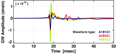
Figure 1: Waveform examples from the DFM gravitational waveform catalog. The amplitudes are for an event at 10 kpc distance from the detector.

II Generation of Event Triggers

In this Section, we overview the target GW signal characteristics, used data, and a burst filter used in this work.

II.1 Target gravitational waves

The target of the analysis in this work is a burst GW from stellar-core collapse (core-collapse supernova explosion). It is difficult to predict its waveform analytically, because of the complex time evolution of the mass densities in the explosion process. Thus, the explosion process and radiated GWs have been investigated by numerical simulations bun-SNwave0 ; bun-SNwave1 ; bun-SNwave2 . Although these simulations were performed with differently simplified models, similar waveforms were obtained in these simulations.

Among these simulations, Dimmelmeier et al. have presented rather systematic surveys on GWs from stellar-core collapses bun-SNwave0 . They have obtained 26 waveforms with relativistic simulations of rotational supernova core collapses, with axisymmetric models with different initial conditions in a differential rotation, an initial rotation rate, and an adiabatic index at subnuclear densities. Although the simulation did not cover all of the initial parameters, we used them as reference waveforms in our analysis, assuming that typical characteristics and behavior of the GWs from stellar-core collapses are included in this waveform catalog.

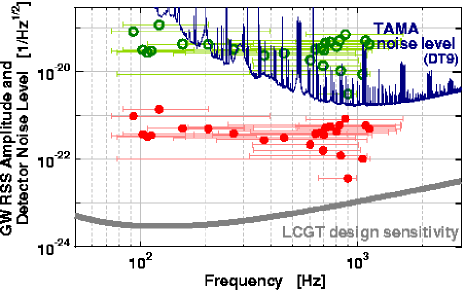
Figure 2: RSS amplitude and center frequency calculated from waveforms in the DFM catalog. The amplitudes are for events at the Galactic center (closed circles), and for events at 100 pc distance from the detector (open circles). Each error bar indicates the frequency range within which the spectrum density value is above half of its peak value. The noise level of TAMA at DT9 and the design sensitivity of LCGT bun-LCGT are shown together.

We processed the original waveforms of the catalog (we call it DFM catalog in this article) with a 30 Hz second-order high-pass digital filter, and resampled them to 20 kHz in order to be compatible with the data from the detector (described in the next part). Figure 1 shows examples from the waveform catalog. While these waveforms have different behaviors, they have common characteristics: about a 1 msec-short spike, and a total duration of less than 100 msec. According to the DFM catalog, the averaged amplitude of GWs radiated by supernovae at the Galactic center (8.5 kpc distance from the detector) is $\langle h_{\rm peak}\rangle=1.5\times 10^{-20}$ in a peak strain amplitude, or $\langle h_{\rm rss}\rangle=4\times 10^{-22}\ [{\rm Hz^{-1/2}}]$ in root-sum-square (RSS) amplitude. Here, a RSS amplitude is defined by

$$h_{\rm rss}=\left[{\int_{-\infty}^{\infty}\left|{h(t)}\right|^{2}\ dt}\right]^{1/2},$$ (1)

where $h(t)$ is the strain amplitude of the GW bun-LIGOburst . The central frequencies of the waves range from 90 Hz to 1.2 kHz (Fig. 2), which is around the observation band of interferometric detectors. Also, it is estimated from the DFM catalog that a total energy radiated as GWs in one event is $\langle E_{\rm tot}\rangle=8\times 10^{-8}\,[M_{\odot}c^{2}]$, in average. Here, $M_{\odot}$ is the mass of the Sun.

II.2 Data from a gravitational wave detector TAMA300

Table 1: Summary of long data-taking runs by TAMA300. The noise level and total observation data amount are described. The last column (D.C.) represents the duty cycle throughout the data-taking run.

	Term	Noise level	Total data	D.C.
		[${\rm Hz^{-1/2}}$]	[hours]
DT6	Aug. - Sept, 2001	$5\times 10^{-21}$	1038	87%
DT8	Feb. - April, 2003	$3\times 10^{-21}$	1157	81%
DT9	Nov., 2003 - Jan., 2004	$2\times 10^{-21}$	558	54%

We applied our analysis method to observation data obtained by TAMA300 bun-TAMA1 ; bun-TAMA3 ; TAMA300 is a Japanese laser-interferometric gravitational wave detector, located at the Mitaka campus of the National Astronomical Observatory of Japan (NAOJ) in Tokyo (${\rm 35^{\circ}40^{\prime}N,\ 139^{\circ}32^{\prime}E}$). TAMA300 has an optical configuration of a Michelson interferometer with 300 m-length Fabry-Perot arm cavities and with power recycling to enhance the laser power in the interferometer. During the operation, the mirrors of the detector are shaken by a 625 Hz sinusoidal signal, which enables us to calibrate the detector sensitivity continuously with a relative error of less than 1% bun-cal . The main output signal of the detector, which would contain GW signals, is recorded with a 20 kHz, 16 bit data-acquisition system bun-daq . Besides the main output signal, over 150 monitor signals are also recorded during the observation: signals for the laser power in and from the interferometer, detector control-loop signals, seismic and acoustic monitor signals, signals for temperature and pressure monitor, and so on ref_DT8 . These monitor signals are used for diagnosing the detector condition, and for veto analyses (Section III). The recorded data are stored in DLT tapes on site, and are sent to data-analysis computers at the collaborating institutes by Giga-bit optical network connections.

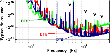
Figure 3: Typical noise level during data-taking runs with the TAMA300 detector. The noise level has been improved run by run. The spectrum contains several line peaks: harmonics of 50 Hz AC power line, violin mode peaks of the suspension wire of the mirror (described as ’V’), and a calibration peak at 625 Hz (described as ’C’).

In TAMA, nine observation runs have been carried out so far since the first observation run in 1999, and over 2700 hours of data have been collected. In this work, we used the data in the sixth, eighth, and ninth data-taking runs (DT6, DT8, and DT9, respectively, Table 1). We obtained over 1000 hours of data in each of DT6 and DT8, operating the detector stably and with a good duty cycle. The duty cycle in DT9 was not very high, because most of the day time was spent for the adjustment and measurement of the detector during the first half term. On the other hand, we obtained data with uniform quality with a high duty cycle in the second half, which included that during the quiet time of new-year holidays. The duty cycle was 96% (207 hours’ observation in 216 hours) in this quiet term of DT9. We used only this stable term as the DT9 data in the following analyses.

Typical noise spectra in these observation runs are shown in Fig. 3. The noise level has gradually been improved by detector investigations between these runs. The detector has a floor-level sensitivity of around from 300 Hz to 2 kHz frequency range. The floor level is $2\times 10^{-21}\,{[\rm Hz^{-1/2}]}$ in DT9 at around 1 kHz. The spectrum contains several line peaks: harmonics of a 50 Hz AC line, violin mode peaks (around 520 Hz and integer multiples) of the suspension wire of the mirror, and a calibration peak. Since these lines could affect the analysis results, they were removed in the data analyses.

II.3 Extraction of signals by an excess-power filter

We developed and implemented a burst-wave analysis code based on an excess-power burst filter. Among several filters proposed so far, an excess-power filter bun-excesspow and a TF-cluster filter bun-TFcluster look for an increase of power in the data of a detector, while a slope filter bun-slope and a pulse correlation filter bun-cor monitor correlations between the data and assumed waveforms. Roughly speaking, a higher detection efficiency is attained with assumptions on the waveform. On the contrary, the efficiency is drastically degraded if there are any errors in the assumed waveforms. An excess-power filter is robust because it uses only a little information on the target waveforms: the signal duration time and the frequency band. The evaluation parameter is the total noise power in a given time-frequency region. In spite of its robustness, it is nearly as efficient as matched filtering for signals with short duration and a limited frequency band bun-excesspow .

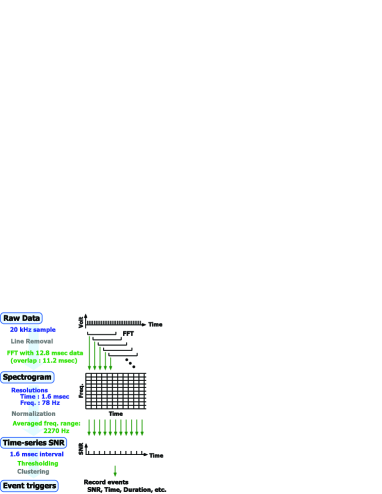
Figure 4: Data-processing chart of our excess-power burst filter. We first calculate a spectrogram from the detector output data. Next, we obtain the time-series SNR by averaging the frequency components. Then, we extract event triggers by a given threshold.

Our filter generates event triggers in the following steps (Fig. 4, details are described in Appendix A): (i) A spectrogram (time-domain change in noise power spectrum) is calculated from the output data of the detector; the power spectrum is calculated with a $\Delta t=12.8$ [msec] data chunk using a fast Fourier transform (FFT), which is repeated with 1.6 msec time-delays. We used a Hanning window in each FFT process to obtain smooth spectra and time-series results. Here, each spectrum has a frequency resolution of $1/\Delta t=78$ [Hz]. Since the original data contains many line peaks (AC line peaks in every 50 Hz, etc.), this low-resolution spectrum is contaminated by these peaks. Thus, these peaks are removed from the original time-series data before calculating the spectrogram. (ii) In each spectrum, power in pre-selected frequency bands are averaged so as to obtain a time-series of averaged power, $P_{n}$. Each spectrum is normalized (whitened) by the typical noise spectrum within 30 min before a calculation of the average in the frequency components. As a result, $P_{n}$ represents the signal-to-noise ratio (SNR): the ratio of the averaged signal power to the typical noise power in pre-selected time-frequency region. In this work, we selected a fixed band of $\Delta f=2270$ [Hz] from 230 Hz to 2.5 kHz. (iii) Event triggers are extracted if the averaged power is larger than a given threshold, $P_{n}\geq P_{\rm th}$. If unusual signals in the detector output are sufficiently large, they will be observed in the filter output. Continuous excesses above the threshold are clustered to be a single event. Each event trigger is recorded with its parameters: the peak signal power $P_{\rm ev}$, the time of the event $t_{\rm ev}$, the duration time above the threshold, and so on.

The parameters of the filter, length of the time chunk ($\Delta t$) for each FFT, and analysis frequency band ($\Delta f$) were selected to be effective for the reference burst GW signals. According to the DFM catalog, the signals have short spike-like waveforms, i.e. a short duration and a wide frequency band. Although the selected parameters ($\Delta t=12.8$ [msec], $\Delta f=2270$ [Hz]) were not fully optimized for the waveforms, the analysis results were not changed very much with a different parameter set. Moreover, we could keep the robustness of the excess-power filter with this rough tuning of the time-frequency bands.

II.4 Signal-injection simulations

Figure 5: Relation of injected signal amplitude and SNR obtained by the injection test for the DT9 data. The asterisk points and the curve represent the signal-injection results and the fitting result, respectively. The points at the lower right side of the plot are caused by waveforms in which the signal power are concentrated at a low-frequency band; the sensitivity of TAMA is worse in these frequency bands (see Fig. 2).

The output of the filter ($P_{\rm ev}$) is a dimensionless signal-to-noise ratio (SNR). SNR is calibrated to a physical value, such as the GW amplitude, by results of signal-injection simulations (called ’software injection tests’) with real data from the TAMA300 detector. In the simulation, target reference waveforms are superimposed to the detector data with proper calibration (estimated from the transfer functions of the detector, the whitening filter, the anti-aliasing filter before the data-acquisition system). The signals are injected and analyzed one by one with equal time separations in the data so as to evaluate the data uniformly. The amplitudes and waveforms were selected randomly from $10^{-22}\leq h_{\rm rss}\leq 10^{-18}\,[{\rm Hz^{-1/2}}]$ and from 26 waveforms in the DFM catalog, respectively. This data were analyzed by the same code as that for the raw data analysis.

The results of the signal-injection test are shown in Fig. 5; the recorded power SNRs of the events ($P_{\rm ev}$) are plotted as a function of the root-sum-square amplitudes of the injected signal ($h_{\rm rss}$). The injection results of each data-taking run were fitted by

$$P_{\rm ev}=1+(C_{{\rm DT}x}\times h_{\rm rss})^{2},$$ (2)

where $C_{{\rm DT}x}$ represent the averaged efficiency coefficients ($x$: the data-taking number). From the injection results, we obtained the coefficient values: $C_{\rm DT6}=2.2\times 10^{19}$, $C_{\rm DT8}=3.3\times 10^{19}$, and $C_{\rm DT9}=8.7\times 10^{19}$.

An inverse of this coefficient corresponds to the GW amplitude with which the signal power is the same as the noise power by our filter. Thus, it is interpreted as the noise-equivalent amplitude of the GW signal. The noise-equivalent GW amplitude was $h_{\rm rss,noise}=1.1\times 10^{-20}\,[{\rm Hz^{-1/2}}]$ for DT9 with our excess-power filter. From the estimation that the averaged GW amplitude was $\langle h_{\rm rss}\rangle=4\times 10^{-22}\,[{\rm Hz^{-1/2}}]$ for a 8.5 kpc event, TAMA has the ability to detect events within around 300 pc away from Earth with this noise-equivalent amplitude.

III Reduction of fake events

In this Section, we describe veto methods to reject fake events caused by detector instabilities. We have used two veto methods: a veto method using auxiliary signals for the detector monitor, and a veto method by the waveform behavior: the time-scale of the signal.

III.1 Veto with auxiliary signals for the detector monitor

Here, we describe a veto method using auxiliary signals recorded together with the main output of the detector: a correlation between the monitor signal and the main output, the confirmation not to reject real GW signals, and a false dismissal rate estimation.

III.1.1 Veto with the intensity monitor signal

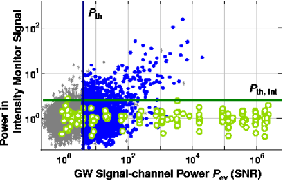
Figure 6: Correlation between the powers in the main output channel and the intensity monitor channel. The closed circles are event candidates selected by the threshold $P_{\rm th}=4$; the gray asterisks are powers at the time 100 msec-shifted from the event candidates, and the open circles are results of hardware-injection tests.

We investigated some of the monitor signals, and found strong correlations between the short spikes in the main output and the monitor signal for the laser intensity in a power-recycling cavity of the interferometer. Figure 6 shows the correlation between the main output and the intensity monitor signal. The intensity-monitor data were processed by the same excess-power filter to detect short-spike instabilities. The filter parameters were the same as that for the main signal analysis, except for the frequency range. In the analysis of the intensity-monitor data, the frequency range was $\Delta f_{\rm int}=1170$ Hz from the DC frequency, which was determined from the spectrum shape of the burst spikes in the intensity data. The closed circles in Fig. 6 represent the power (SNR) of the events in the GW data-channel and in the intensity monitor. In this figure, the event triggers were extracted with a threshold of $P_{\rm th}=4$ for the DT8 data. For a comparison, the powers at the time 100 msec-shifted from the triggers are also plotted in this figure (gray asterisks) . This figure shows that there are strong correlations between these two signal powers for some of the event triggers, and only weak correlations outside of the event triggers.

Thus, vetoes of fake events with the intensity monitor signal are expected to be effective; when the outputs of two excess power filters (one for the GW signal-channel, and another for the intensity monitor) exceed the respective thresholds simultaneously, the triggers are labeled as fakes, and are removed from the event candidate list.

III.1.2 Estimation of a false-dismissal rate

To use the veto with the intensity monitor signal, we should confirm that the intensity instabilities were not caused by huge GW signals; otherwise, we may reject real GW signals by this veto. During DT8, we investigated the response of the detector by injecting simulated waveforms to it. In this test, which is called a ’hardware injection’ test, we shook the interferometer mirrors with a short-spike waveform and a typical burst-waveform obtained by numerical simulations bun-SNwave1 with various amplitudes. The results of the hardware-injection test are plotted as open circles in Fig. 6. There were 147 injections, and 117 events were above the event-selection threshold of $P_{\rm th}=4$. We observed no excess power in the intensity monitor with an intensity veto threshold of $P_{\rm th,int}=2.2$ (described below), while the injected signals appeared with sufficiently large powers in the filter output for the GW signal-channel. The number of accidental excesses with this threshold is expected to be 1.2 (1% of injected events). Thus, the result that no excess was found above the intensity threshold is well-consistent with the expected accidental background. From these results, we ensured that the intensity instabilities were not caused by huge GWs, and that it is safe to use the intensity monitor signal for a veto analysis.

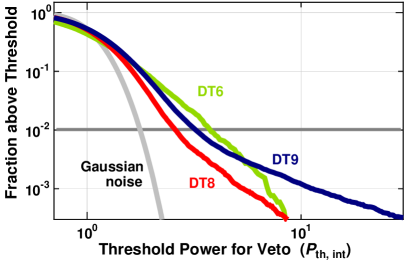
Figure 7: Estimation of an accidental coincidence. The intensity-veto threshold was decided so that the accidental coincidence probability (or the false-dismissal rate in this case) would be 1%. As a result, the thresholds are $P_{\rm th,int}=3.9$, 2.2, and 3.0 for DT6, DT8, and DT9, respectively.

The threshold for the intensity excess power is selected so as to reduce fake events effectively with small probability to reject real GW signals, i.e. with a small false-dismissal rate. The false-dismissal rate is equal to the accidental coincidence rate between the intensity excess and the excess in GW signal-channel, which was estimated from the distribution of the power in the intensity monitor signal. We selected a threshold so that the false-dismissal rate would be 1%, which resulted in thresholds of $P_{\rm th,int}=3.9$, 2.2, and 3.0 for DT6, DT8, and DT9, respectively (Fig. 7). The difference in the thresholds for these data-taking runs were caused by the difference in the detector stability in each run and the improvement of the intensity monitor instrument between DT8 and DT9.

III.2 Veto by a signal behavior test

Here, we describe the second veto method, a veto method by the time-scale of the signal. Statistics for the signal evaluation, and an estimation of the false-dismissal rate are described.

III.2.1 Signal behavior test

As described above, fake events are rejected by careful selection and an investigation of the monitor signal-channels. However, it is hard to see any clear correlations for all of the fake events in practice, because there are various origins of the fakes, which are difficult to be identified. Thus, a test of the signal behavior at the main output of the detector will be helpful to reduce fake events.

The effectiveness of the veto with a signal behavior test depends on how well we know, or how many assumptions we set, on the signal behavior. In the burst-wave analysis case, the waveforms by numerical simulations suggest that GWs from stellar-core collapse have a short duration, typically less than 100 msec. We know that some of the detector instabilities last longer than a few seconds from experience. Thus, some of the fakes caused by these slow instabilities are rejected by evaluating the time scale of the event triggers ref_ngnr .

III.2.2 Evaluation statistics for the time-scale veto

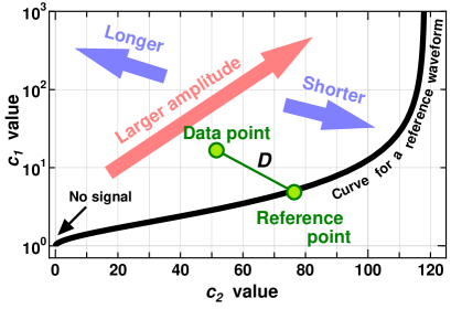
Figure 8: Evaluation of a data point on a $c_{2}$-$c_{1}$ correlation plot. The curve shows the expected locus for a reference waveform, which was drawn by sweeping the signal amplitude. The distance between a data point and a reference point on the reference curve represents the similarity of the signal amplitudes and their time scales.

In this work, we selected to evaluate the time scale of event triggers with statistics around the event (Appendix B for details). The excess-power filter outputs $P_{n}$, a time series of the power in a pre-selected frequency band. We calculate two statistics from the $\pm\Delta T/2$ time-series data around the event-candidate time $t_{\rm ev}$:

$$c_{1}=Q_{1}\ \ \ {\rm and}\ \ \ c_{2}={1\over 2}\left({{Q_{2}\over Q_{1}^{2}}-1}\right),$$ (3)

where $Q_{k}=\sum P_{n}^{k}/N$ ($k$: integer) is the $k$-th-order moment of the power bun-kur ; bun-NRC . Here, $N$ is the number of power-data points in the evaluation time (within $t_{\rm ev}\pm\Delta T/2$). The statistics $c_{1}$, which is related to an averaged power, has information about the stability of the noise level on a given time scale. On the other hand, $c_{2}$ is related to the second-order moment of the noise power. Since it is normalized by the averaged power ($Q_{1}$), the $c_{2}$ value becomes constant if the signal power is much larger than the background noise level. The constant number is determined by the time scale of the event: large in a short-burst case, and small in a case of a slow change in the noise power.

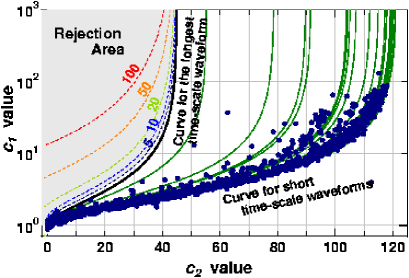
Figure 9: Correlation plot of $c_{1}$ and $c_{2}$ used for the rejection of fake events, calculated with a time window of $\Delta T=0.82$ [sec]. The solid curves show the expected loci for the reference waveforms from the DFM catalog. Among them, the curve for the waveform with the longest time-scale is shown as a bold curve. The dotted curves represent the contours for the distance $D_{\rm min}$ to the longest time-scale reference curve. When event triggers are in the gray area, which is the $D_{\rm min}\geq 5$ area, they are rejected as fakes. The closed circles represent the results of the signal-injection test using the data of DT9. With a fake-event-selection threshold of $D_{\rm th}=5$, the false dismissal rate was estimated to be 0.3%.

We use an evaluation parameter ($D_{\rm min}$), which represents the similarity to the GW signal, estimated from the $c_{1}$ and $c_{2}$ statistics. When we plot the data point in the $c_{2}$-$c_{1}$ plane (Fig. 8), they will be in the left region for long-duration event cases and in the right region for short burst-like event cases, and will be in the upper region for large power events. Thus, two independent information on each event, the power and the time scale, are shown by the position of each data point in this plot. Here, the distance ($D$) between the data point and a reference point (expected position of the real GW signal, estimated from the signal waveform), represents the similarity of their signal behaviors. The evaluation parameter ($D_{\rm min}$) is the smallest distance for all of the reference waveform and amplitude combinations.

In a practical application of this method to real data, we set a loose selection criteria for fake events (Fig. 9). We have 26 reference GW waveforms from the DFM catalog, which have different time scales. Instead of comparing the time scale of an event trigger with that of each reference waveform, we compare it only with the longest time scale of the reference GW waveforms. In other words, the evaluation parameter of an event ($D_{\rm min}$) is set to be zero if its time scale is shorter than that of the longest reference waveform.

III.2.3 Selection of parameters for the time-scale veto

Fake events with different behaviors from that of the real ones are rejected when the minimum distance ($D_{\rm min}$) is larger than a given threshold ($D_{\rm th}$). Here, two parameters should be set in this veto analysis: an evaluation time-window ($\Delta T$) and a fake-selection threshold ($D_{\rm th}$). The time window is selected to be $\Delta T=0.82$ sec, so that the veto would be effective. Since this time window length is between the typical time scales of the fakes (larger than a few seconds) and the real GW signals (less than 100 msec), we can expect a clear distinction between them. On the other hand, the threshold for the rejection ($D_{\rm th}$) is selected so that the false-dismissal rate of real GW signals would be acceptable.

The false-dismissal rate was directly evaluated from the results of a signal-injection test with the real data from the TAMA300 detector (described in Sec. II.4). This simulation is important because the real data from a detector do not have an ideal Gaussian noise distribution. The closed circles in Fig. 9 show the results of the signal-injection test to the DT9 data. The injection results are distributed well-around the theoretical predictions shown as solid curves. With a fake-event-selection threshold of $D_{\rm th}=5$, the false-dismissal rate was estimated to be 0.3%; 6 injection results were rejected out of 2006 injections . Although this value is larger than that estimated by a statistical analysis, it is sufficiently small for a veto analysis. The false dismissal rates were also investigated for the DT6 and DT8 data with a similar signal-injection test, and found to be 0.6% and 2.9%, respectively. The differences come from the original behavior of the data in these observation terms.

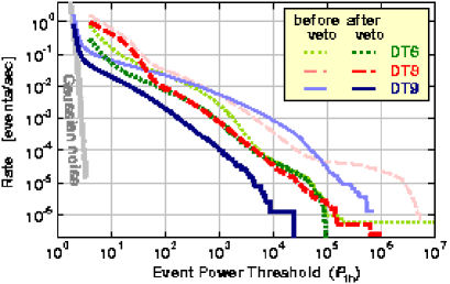
Figure 10: Event-trigger rate results with TAMA data. The horizontal and vertical axes represent the threshold ($P_{\rm th}$) and the trigger rate in a unit of events/sec, respectively. The analysis result with simulated Gaussian noise is also plotted together with the DT6, DT8, and DT9 results.

IV Data-processing results with the TAMA300 data

The analysis method described above was applied to real data from TAMA300. In this section, we consider the results of the TAMA data analysis with the vetoes, and the interpretation of the results from an astronomical point of view. The data were mainly processed by a PC-cluster computer placed at the University of Tokyo. This machine is comprised of 10 nodes, and has 20 CPUs (Athlon MP 2000+ by AMD Inc.). The analysis time for the excess power filter was about 30-times faster than the real time; it took about 1/30 sec to process 1-sec data.

In the data processing, the first 9-min and the last 1-min data of the each continuous observation span were not used because they sometimes contained loud noises caused by detector instabilities, or excited violin-mode fluctuations. In addition, the duration time of rejected fake events is considered as a dead time of the detector, and subtracted from the total observation times. The dead times by the fake rejections were 1.3%, 1.7%, and 0.4% of the observation time for DT6, DT8, and DT9, respectively. The effective observation times ($T_{\rm obs}$) are shown in Table 2.

IV.1 Event-trigger rates

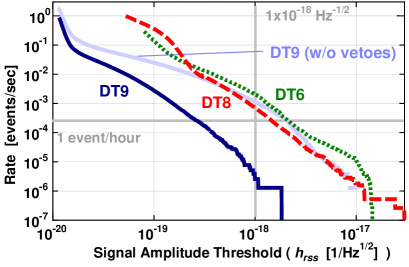
Figure 11: GW amplitude and corresponding trigger rate; the event rate (vertical axis) with larger amplitude than a given $h_{\rm rss}$ (horizontal axis) is plotted.

Figure 10 shows the event-trigger rates obtained by the TAMA data analyses; the trigger rate (in a unit of events/sec) is plotted as a function of the event-extraction threshold ($P_{\rm th}$). The analysis result with simulated Gaussian noise is also plotted in Fig. 10, together with the DT6, DT8, and DT9 results. Assuming that the real GW signals are rare and faint, we can regard most of the triggers as being fakes. From this figure, one can see that the trigger rates were reduced in these data-taking runs with vetoes. For a given GW power threshold ($P_{\rm th}$), the trigger rates were reduced by 1/10-1/1000. The power threshold could be reduced (for better GW-detection efficiency) by a factor of 10-100 for a given trigger rate. Figure 11 shows the event-trigger rates plotted as a function of $h_{\rm rss}$ amplitude, which was obtained from Eq. (2). The detector was gradually improved during the intervals of these data-taking runs. The event-trigger rates were reduced from DT6 to DT9 by about a few orders for a given GW amplitude, and by about an order for given trigger rates (Table 2).

Table 2: Summary of data analysis results. The noise-equivalent GW RSS-amplitudes ($h_{\rm rss,noise}$), the dead times by the vetoes ($T_{\rm rej}$), the total effective observation times ($T_{\rm obs}$), the trigger rates for $h_{\rm rss}\geq 1\times 10^{-18}\,[{\rm Hz^{-1/2}}]$, and the GW RSS-amplitudes above which the trigger rates are one event per hour are described.

	$h_{\rm rss,noise}$	$T_{\rm rej}$	$T_{\rm obs}$	Rate	1-${\rm hour^{-1}}$ amp.
	[${\rm Hz^{-1/2}}$]	[hours]	[hours]	[${\rm sec^{-1}}$]	[${\rm Hz^{-1/2}}$]
DT6	$4.5\times 10^{-20}$	11.8	937.8	$2.1\times 10^{-3}$	$2.1\times 10^{-18}$
DT8	$3.0\times 10^{-20}$	18.0	1064.2	$7.0\times 10^{-4}$	$1.4\times 10^{-18}$
DT9	$1.1\times 10^{-20}$	0.8	194.6	$2.5\times 10^{-6}$	$2.5\times 10^{-19}$

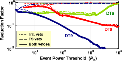
Figure 12: Reduction factor by two veto methods for DT6, DT8, and DT9. The bold curves are the reduction ratio with two vetoes. The dotted and dashed curves are only with an intensity veto and a time-scale veto, respectively.

Figure 12 shows the reduction factor of event triggers with two veto methods; the ratio of the number of event triggers after and before the vetoes are plotted as a function of the SNR threshold. In these runs, both of the two vetoes contributed to the reduction of the rates. They worked in complementary ways. The intensity veto is effective to short-duration fakes and large SNR fakes. On the other hand, the time-scale veto is effective for the long-time instability of the detector output and small SNR fakes.

In DT9, many event triggers were rejected as fakes by the intensity veto. This is because the pre-amplifier and whitening filter for the data acquisition of the intensity signal were improved in this run. Since the reduction factor is better for large SNR fakes, it is expected that the reduction ratio will be further improved with a higher detection efficiency of the intensity instabilities. On the other hand, only a small fraction of fakes were rejected by the time-scale selection in DT9 because the detector operation was sufficiently stable. The detector was operated very stably thanks to a quiet seismic environment during the holiday weeks in the second half of DT9. In addition, the drift of the typical noise level was small at that time. In DT6, the time-scale veto was much more effective than the intensity veto. This is because DT6 data contained noisy data originating in an instability of the laser source and seismic disturbances during the daytime.

The rates are still much larger than that with simulated Gaussian noises, even with the vetoes and the improvements in the detector. In addition, the trigger rate is still much higher than the expected rate of supernova explosions. The expected GW event rate is one event in a few tens of years, i.e. about $10^{-9}$ events/sec in our Galaxy. (Here, note that TAMA has an ability to detect only events within 300 pc away from Earth at best.) These results suggest that most of the observed trigger-events were fake events caused by an instability of the detector, even with vetoes.

IV.2 Simulations of Galactic events

Since the event-trigger rate is still much larger than that expected from ideal Gaussian noise or observed supernova rates, we cannot claim the detection of GW signals from the data-analysis results. Thus, we set upper limits for stellar-core collapse events in our Galaxy. We carried out Monte-Carlo simulations with a source-distribution model of our Galaxy, and with waveforms from the DFM catalog. The simulated data were analyzed in the same way as the detector data, and compared with the observation results.

In the simulation, we adopted a source-distribution model based on the observed luminous star distribution in our Galaxy, assuming that the event distribution of the stellar-core collapses was identical to it. There have been studies on the star-distribution model based on sky-survey observations ref-galmod1 ; ref-galmod2 . In our simulation, we used a simple axisymmetric distribution model (an exponential disk model) described in a cylindrical coordinates,

$$\rho(R,\theta,z)\propto\exp\left({-{R\over R_{0}}-{|z|\over h_{0}}}\right),$$ (4)

where $\rho$, $R_{0}=3.5$ kpc, and $h_{0}=320$ pc are the density of the events, and the characteristic radius and height of the density of the Galactic disk, respectively. As well as the non-axisymmetric components, such as spiral arms, the thick disk and halo structures were neglected in our simulations because their number of stars was only about 3% of that of the disk component ref-galmod2 . We adopted $R_{\odot}=8.5$ kpc and $h_{\odot}=20$ pc for the position of the Sun in our simulation.

We used 200 hours stable data in the second half of DT9 for the Galactic signal-injection test. This test was performed according to the following steps: (i) Set the GPS times at which simulated events are injected; these times are uniformly separated between the start and end times of the observation run. Decide the position of each event randomly according to the Galactic-event distribution described by Eq. (4). Select the waveform of each event randomly from the DFM catalog. (ii) Calculate the distance and sky direction seen from the detector for each event, from the position of the event in the Galaxy and the injection time information. (iii) The expected GW amplitude is calculated from the distance to the event source and the detector antenna pattern for the sky position of the event . We assumed non-polarized GWs; the GW power is equally distributed to the two polarizations. (iv) Inject each event waveform to the TAMA300 data with estimated amplitude, and analyze the data with a similar code as that for the raw-data analysis. (v) Extract the events at the injected time.

IV.3 Results of Galactic-event simulations

Figure 13 shows the results of a Galactic-event simulation. The fraction of the detectable Galactic events (the detection efficiency, $\epsilon_{\rm gal}$, left axis) is plotted as a function of the SNR threshold ($P_{\rm th}$). The event-trigger rate in DT9 is also plotted for a comparison (right axis). With an event-selection threshold of $P_{\rm th}=3.0$ (which corresponds to averaged amplitude of $h_{\rm rss,th}=1.6\times 10^{-20}\,[{\rm Hz^{-1/2}}]$ for DT9), the detection efficiency was estimated to be $\epsilon_{\rm gal}=3.1\times 10^{-5}$ for the Galactic events. The threshold was selected so that the expected contribution of the Gaussian noise would be sufficiently small (less than 1% of the triggers above the threshold). The upper limit for the event rate determined from the TAMA raw-data was $R_{\rm DT9,UL}=6.8\times 10^{-2}$ events/sec with a confidence level of 90%. From these results, we obtained the upper limit for the Galactic event rate to be $R_{\rm gal,UL}=R_{\rm DT9,UL}/\epsilon_{\rm gal}=2.2\times 10^{3}$ [events/sec] with a 90% confidence level . This value is considerably larger than the theoretical expectation of about $10^{-9}$ events/sec.

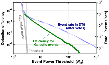
Figure 13: Results of a Galactic-event simulation. The solid curve shows the detection efficiency for the Galactic events as a function of the threshold. The trigger rate obtained by the DT9 observation is also plotted as a dotted curve for a comparison (right vertical axis).

Besides the upper limit for the rate of a stellar-core collapse in our Galaxy, an upper limit was set for the GW energy rate. The total energy radiated as GW, $E_{\rm tot}$, was estimated for each event from its waveform. The upper limit for the energy rate radiated as GW was estimated by the product of the event-rate upper limit, $R_{\rm gal,UL}$, and the averaged GW energy of the events, $\langle E_{\rm tot}\rangle$. As a result, we obtained $\dot{E}_{\rm GW,UL}=3.8\times 10^{-4}\,[M_{\odot}c^{2}$/sec]. Again, this value is considerably large; the rate of the total energy radiated as GWs would be about $M_{\rm Gal}/(2\times 10^{7})\,[M_{\odot}c^{2}$/years], where $M_{\rm Gal}$ is the total mass of our Galaxy, which we assume to be $2\times 10^{11}\,M_{\odot}$.

There are uncertainties in setting the upper limits by several origins. Here, we consider the effect of the detector calibration error, statistical error in the Monte-Carlo simulation for the Galactic events, and the error in the Galactic model. The calibration error in the conversion of the detector output to the GW strain amplitude was estimated to be less than 1%. This calibration error causes an amplitude error in the signal-injection test. From Eq. (2) and the results of the Galactic signal-injection test, the uncertainty in the upper limit is estimated to be 2.9% with a detector calibration error of 1%. On the other hand, the statistical error in the Monte-Carlo simulation is determined by the number of the simulated events above the threshold. We generated $3.8\times 10^{8}$ Galactic events, and detected $1.2\times 10^{4}$ events above the threshold of $P_{\rm th}=3.0$. Assuming that the number of detected events follows a Poisson distribution, the event-rate uncertainty is 0.9%. At last, the error in the Galactic model would affect the results. The parameter $R_{0}$ in the Galactic model has an error of 9.4% ref-galmod2 . This error corresponds to a 5.8% uncertainty in the detection efficiency for the Galactic events ($\epsilon_{\rm gal}$) with a threshold of $P_{\rm th}=3.0$, which was estimated by additional simulations. In total, the uncertainty in our upper-limit results is 6.5% at most. The detection efficiency will be reduced (the upper limit will be increased) by 1.2% by including a thick disk and halo components.

V Discussions

V.1 Comparison with previous studies

We interpreted the observation results from the viewpoint of the Galactic event rate in the previous section. In this part, we interpret the results in an similar way as in the previous studies for a comparison; we set an upper limit on the rate of GW events incident on the detector as a function of the GW amplitude bun-LIGOburst ; bun-IGECburst .

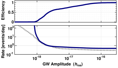
Figure 14: Detection efficiency and an upper limit (90% confidence level) for the waveforms of the DFM catalog. The detection efficiency with a given threshold of $P_{\rm th}=10^{4}$ is shown in the upper plot, and the upper limit on the event rate is shown in the lower plot (solid curve). The gray dotted curve is the envelope of the upper limits with various detection thresholds.

We used 200 hours of data in the DT9 stable term, and set an upper limit on the rate of the events received by the detector, following the procedure to set the upper limits by the LIGO group bun-LIGOburst . At first, the detection threshold was fixed, and the upper limit was set at the number of the events above the threshold with a given confidence level. Then, the detection efficiency for a given GW amplitude was estimated by a software signal-injection test. Here, the events were distributed randomly on the celestial sphere in order to include the directivity of the detector. We investigated the Gaussian (with a time scale of $\tau=0.5$ and 1 [msec]) and sine-Gaussian waveforms (with Q-value of 9 and central frequencies of 554, 850, and 1304 Hz) for a comparison with the previous studies, as well as the waveforms from the DFM catalog. Finally, we estimated the upper limit on the event rate from the upper limit on the number of events, $N_{\rm UL}$, the detection efficiencies, $\epsilon$, and the observation time, $T_{\rm obs}$, by $R_{\rm UL}=N_{\rm UL}/(\epsilon\cdot T_{\rm obs})$.

We set the threshold to be $P_{\rm th}=10^{4}$, which resulted in one trigger above the threshold. Assuming Poisson statistics, we obtained the corresponding upper limit of 3.89 events with a confidence level of 90%. The detection efficiencies and the upper limit results are shown in Fig. 14 (waveforms from the DFM catalog) and Fig. 15 (Gaussian and sine-Gaussian waveforms).

The upper limit for sufficiently large events (ex. $h_{\rm rss}>1\times 10^{-16}\,[{\rm Hz^{-1/2}}]$) was 0.49 events/day with a confidence level of 90%. This upper limit is comparable to the LIGO-S1 result of 1.6 event/day bun-LIGOburst and the Glasgow-MPQ coincidence result of 0.89 events/day bun-coin1 . On the other hand, the resonant detector network has set an upper limit of $\sim 4\times 10^{-3}$ events/day bun-IGECburst . These differences in the upper limits come mostly from the different observation times. As for the sensitivity for smaller amplitude signals, the GW amplitude for 50% detection efficiencies (averaged over source directions) was around $1\times 10^{-18}\,{\rm Hz^{-1/2}}$ for short and high-frequency waveforms in our case. The upper limit curve is almost comparable with the LIGO-S1 results for high-frequency signals, and larger for lower frequency ($<$ 800 Hz) ones bun-LIGOburst .

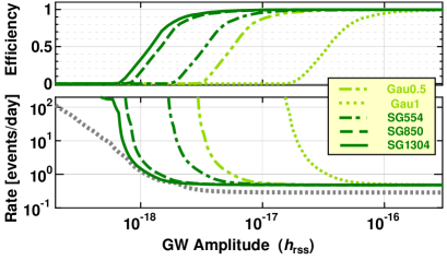
Figure 15: Detection efficiencies and upper limits (90% confidence level) for the Gaussian (time scale of 0.5 and 1 msec) and sine-Gaussian (central frequency of 554, 850, and 1304 Hz) waveforms. The gray dotted curve is the envelope of the upper limits for the 1304 Hz sine-Gaussian waveform with various detection thresholds.

V.2 Outlook for the detection of burst GWs

The large event rate and upper limit results show that the detector output is still dominated by fake events, even after these vetoes. Thus, further research efforts are necessary to detect burst gravitational waves. In this part, we discuss the outlook to better vetoes, coincidence analyses with other observatories, and better performance of the detector and data-processing scheme.

In Section III.1, we presented a veto analysis method with only one monitor signal, an intensity monitor. Similar methods can be used with the other monitor signals along with careful investigations of their correlations with the main output of the detector. However, we have found no other monitor signal with a clear correlation so far: laser power at the signal-port (the dark port), monitors for the seismic fluctuations, an acoustic monitor signal. Thus, it is necessary to investigate more deeply the monitor signals, and to introduce better monitor signals that are sensitive to the detector instabilities.

There are other event-selection criteria than the time-scale selection method presented in Section III.2. For example, the time scale of an event can be simply evaluated by the duration time above the event-selection threshold. In this case, we should consider that the veto results will be strongly dependent on the event amplitude . We will be able to reduce fake events even further by knowing the common characteristics of the target events, and setting them as event-selection criteria. For this, more systematic and precise simulations of stellar-core collapses and investigation on the waveform will be helpful.

Coincidence analyses with the other detectors for GWs, electromagnetic waves, and neutrinos will improve the result significantly, though we have focused on the reduction of fakes with a single detector in this article. The observation runs by TAMA300 (DT8 and DT9) were carried out at the same term as the LIGO second and third scientific (observation) runs (called S2 and S3), and coincidence analyses are underway bun-coinLIGO . We note that our work discussed in this article is also a part of the LIGO-TAMA coincidence analysis; the list of the event triggers obtained in our work will be used in the coincidence analysis.

In addition to a reduction of fakes, the improvements of the detector both in the floor noise level and in the reduction of non-stationary noises are also important. The performance of the TAMA300 detector has gradually been improved from DT6 to DT9 concerning both the noise level and the stability, and the detector still has room for improvement. In addition, burst filters with higher efficiencies are under development in the TAMA group and other groups. Since we can only observe events within about the 300 pc range with the current sensitivity of TAMA, the detection efficiency for the Galactic events is very small ($\epsilon_{\rm gal}=8.9\times 10^{-5}$ with a threshold for a noise-equivalent GW amplitude). The sensitivity should be improved by about two orders so as to cover our Galaxy, and to realize a sufficiently large detection efficiency. This sensitivity will be realized by the next-generation detectors, such as LCGT (Fig. 2) bun-LCGT and advanced LIGO bun-AdLIGO .

VI Conclusion

We presented data-analysis schemes and results of observation data by TAMA300, targeting at burst signals from stellar-core collapses. Since precise waveforms are not available for burst gravitational waves, the detection schemes (the construction of a detection filter and the rejection of fake events) are different from those for chirp wave analyses. We investigated two methods for the reduction of non-stationary noises, and applied them to real data from the TAMA300 interferometric gravitational wave detector. As a result, these veto methods, a veto with a detector monitor signal and a veto by time-scale selection, worked efficiently in a complimentary way. The former and the latter were effective for short-spike noises and for slow instabilities of the detector, respectively. The fake-event rate was reduced by a factor of about 1000 in the best case.

The obtained event-trigger rate was interpreted from the viewpoint of the burst gravitational-wave events in our Galaxy. From the observation and analysis results, we set an upper limit for the Galactic event rate to be $2.2\times 10^{3}$ events/sec (confidence level 90%), based on a Galactic disk model ref-galmod2 and waveforms obtained by numerical simulations of stellar-core collapses bun-SNwave0 . In addition, we determined the upper limit for the rate of the energy radiated as gravitational-wave bursts to be $3.8\times 10^{-4}\,M_{\odot}c^{2}$/sec (confidence level 90%). These large upper limits show that the detector output was still dominated by fake events, even after the selection of events, and gives us prospects on both current and future research: the necessity for further improvement of the analysis schemes, coincidence analyses with multiple detectors, better predictions on the waveforms, and future detectors, such as LCGT and advanced LIGO, to cover the whole of our Galaxy. This work has set, we believe, a milestone for these research activities.

Appendix A Detailed description on the excess-power filter

A.1 An excess-power filter

In this part, we detail the excess-power filter. We assume that the output of a detector is comprised of an ideal stationary Gaussian noise, $n(t)$, and a signal, $s(t)$ (non-Gaussian component caused by gravitational waves or instability of the detector): $v(t)=n(t)+s(t)$. The power spectrum is calculated for every $\Delta t$ data chunk with given time-delays ($\delta t$), using a fast Fourier transform (FFT). As a result, we obtain a spectrogram (a time-frequency plane) of the noise (or signal) power with $\delta t$ time separation and $1/\Delta t$ frequency resolution. Here, the Fourier component is also described by the sum of the noise and the signal: $\tilde{v}_{mn}=\tilde{n}_{mn}+\tilde{s}_{mn}$, where $m$ and $n$ represent the indices for the frequency and time, respectively. Then, the power in each time-frequency component is described by $|\tilde{v}_{mn}|^{2}$.

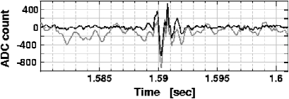
Figure 16: Example of the line removal results for the DT9 data. Time-series data before (plotted in gray) and after (plotted in black) the line removal are shown. The lower plot is a zoom up of the spike in the upper plot.

In order to make our filter equally effective for all of the analysis frequencies, we normalize the power spectrum by an averaged noise level, $\overline{N_{m}}=\sum_{n=n_{0}}^{n_{0}+N_{\rm av}-1}|\tilde{n}_{mn}|^{2}/N_{\rm av}$, where $N_{\rm av}$ is the number of time components used for the average. Then, the normalized power is written as

$$P_{mn}=N_{mn}+2C_{mn}+S_{mn},$$ (5)

where $N_{mn}=|\tilde{n}_{mn}|^{2}/\ \overline{N_{m}}$, $S_{mn}=|\tilde{s}_{mn}|^{2}/\ \overline{N_{m}}$, and $C_{mn}=\Re\{\tilde{s}_{mn}\cdot\tilde{n}_{mn}^{*}\}/\ \overline{N_{m}}$, meaning a normalized noise power, a normalized signal power, and a normalized correlation between the signal and noise components, respectively. Since $\tilde{n}_{mn}$ has a Gaussian noise distribution, $N_{mn}$ has a $\chi^{2}$ distribution of two degrees of freedom (an exponential distribution): $P(N_{mn})=\exp({-N_{mn}})$.

Then, the output of the excess-power filter, the averaged power for a given time component, is written as

$$P_{n}={1\over M}\sum_{m}P_{mn},$$ (6)

where $M$ is the number of frequency components used in the average; only the values of the power in pre-selected frequency components are used to calculate the averaged power, $P_{n}$. From Eq. (5), $P_{n}$ is written as

$$P_{n}=N_{n}+2C_{n}+S_{n},$$ (7)

where $N_{n}\equiv\sum_{m}N_{mn}/M$, $C_{n}\equiv\sum_{m}C_{mn}/M$, and $S_{n}\equiv\sum_{m}S_{mn}/M$. This represents the time evolution of the power in detector output in given frequency bands.

A.2 Data conditioning

The data from the detector is not an ideal Gaussian noise, in practice; the noise spectrum is not white, the noise level changes in time, and many line peaks are included in the output. Thus, data conditioning before processing the excess power filter is indispensable.

The spectrum contains several line peaks: harmonics of 50 Hz AC line, violin mode peaks (around 520 Hz and integer multiples) of the suspension wire of the mirror, and a calibration peak. These line peaks are removed in the following processes. At first, we obtain a Fourier spectrum from 72 sec of data by FFT. We then set the line-frequency components to be zero. In addition, the lower frequency components below 160 Hz are also rejected. At last, we obtain a time-series data by calculating the inverse FFT of the spectrum. With this process, the line peaks are clearly removed from the spectrum (Fig. 16, 17). Moreover, since only a small number of frequency components are rejected, the burst waveforms are not vary much affected by the line removal process.

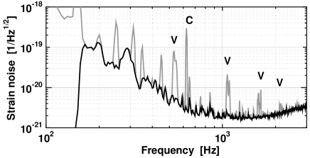
Figure 17: Results of line removal for the DT9 data. The noise spectrum before (plotted in gray) and after (plotted in black) the line removal are shown.

The frequency and time dependences of the noise spectrum are compensated by the normalization with the averaged noise power spectrum, $\overline{N_{m}}$. We calculated $\overline{N_{m}}$ by averaging the power spectra for 30 min before the data analyzed by the excess-power filter. In order to avoid the large spikes from disturbing the averaged spectrum, we rejected noisy 0.7% spectra from those used in each average. We found that we could obtain stable averaged spectra, and that each spectrum was normalized well with this method.

Appendix B Time-scale evaluation and veto

B.1 Evaluation in $\Delta$T time chunk

In this part, we describe the details of the veto method with time-scale evaluation of the event triggers. In our veto methods, each event is evaluated by the statistics in a $t_{\rm ev}\pm\Delta T/2$ data chunk ($t_{\rm ev}$: the time of the event). Here, $N$ data points of the excess-power-filter output are contained in the time window $\Delta T$, i.e. $\Delta T=N\delta t$. From the output of the excess-power filter, $P_{n}$, we define the evaluation parameters $c_{1}$ and $c_{2}$ as

$$c_{1}\equiv Q_{1},\ \ \ c_{2}\equiv{Q_{2}\over Q_{1}^{2}}-1,$$ (8)

where $Q_{1}$, and $Q_{2}$ are the first- and second-order moments of $P_{n}$ for $N$ data points, respectively, written as:

$$Q_{1}\equiv{1\over N}\sum_{n=n_{0}}^{n_{0}+N-1}P_{n},\ \ \ Q_{2}\equiv{1\over N}\sum_{n=n_{0}}^{n_{0}+N-1}(P_{n})^{2}.$$ (9)

Here, note that $Q_{1}$ is an averaged power for $M\times N$ time-frequency components. On the other hand, $c_{2}$ is defined by the second-order moment normalized by the averaged power. This value is analogous to the kurtosis (defined by the fourth-order moment of data), which describes any non-Gaussianity of the data bun-kur ; bun-NRC .

B.2 Statistics of $Q_{1}$ and $Q_{2}$

We calculate the statistics of parameters $Q_{1}$ and $Q_{2}$ as a preparation for calculating the statistics of the parameters $c_{1}$ and $c_{2}$, defined in Eq. (8). Although the $M\times N$ components are not independent in practice, because of overlapping in time and a window function, we describe the following calculations while assuming that they are independent, for simplicity. In practical use, the statistics (the averages, the variances, and the covariance) are estimated by replacing the time and frequency window size, $N$ and $M$, by effective time and frequency range, $N_{\rm eff}$ and $M_{\rm eff}$. The effective window sizes, $N_{\rm eff}$ and $M_{\rm eff}$, are estimated by simulations with Gaussian noises.

From Eq. (7), $Q_{1}$ is also written by the sum of the noise, signal, and their correlation terms. Thus, the expected value is

$$E(Q_{1})={1\over N}\sum_{n}\left\{{S_{n}+E(N_{n})+2E(C_{n})}\right\}=\alpha+1,$$ (10)

where we define the average of the signal component power by

$$\alpha\equiv{1\over N}\sum_{n}S_{n},$$ (11)

and we use relations $E(N_{n})=1$ and $E(C_{n})=0$. The expected value of the square of $Q_{1}$ is written as

$$E(Q_{1}^{2}) = E\left({{1\over N^{2}}\sum_{j}\sum_{l}\left({S_{j}+N_{j}+2C_{j}}\right)\left({S_{l}+N_{l}+2C_{l}}\right)}\right)$$

$$= {2\alpha+1\over MN}+(\alpha+1)^{2},$$

where we use relations $E(N_{k}N_{l})=E(N_{k})E(N_{l})$ $(k\neq l)$, $E(N_{n}^{2})=(M+1)/M$, and so on. Thus, the variance of $Q_{1}$ is written as

$$\mu_{2}(Q_{1})=E(Q_{1}^{2})-E(Q_{1})^{2}={(2\alpha+1)\over MN}.$$ (12)

On the other hand, the expected value of $Q_{2}$ is

$$E(Q_{2}) = E\left({{1\over N}\sum_{n}\left({S_{n}+N_{n}+2C_{n}}\right)^{2}}\right)$$ (13)

$$= \beta_{2}\alpha^{2}+2\alpha+1+{2\alpha+1\over M},$$

where $\beta_{2}$ is a constant value related to the second-order moment of the signal,

$$\beta_{2}\alpha^{2}=\sum_{n}S_{n}^{2}/N.$$ (14)

Similarly, a constant value, $\beta_{3}$, is written as $\sum_{n}S_{n}^{3}/N=\beta_{3}\alpha^{3}$. The constant numbers $\alpha$, $\beta_{2}$ and $\beta_{3}$ are determined only by the waveform and the amplitude of the signal. The value $\alpha$ represents the normalized signal power. The value $\beta_{2}$ depends on the time scale of the signal; $\beta_{2}$ becomes large for a short signal.

With more complicated, but similar, calculations, the variance of $Q_{2}$ and the covariance between $Q_{1}$ and $Q_{2}$ are obtained to be

$$\mu_{2}(Q_{2}) = {8\over N}\beta_{3}\alpha^{3}+{20M+32\over M^{2}N}\beta_{2}\alpha^{2}$$

$$+{16(M^{2}+M+3)\over M^{3}N}\alpha$$

$$+{2(2M^{2}+5M+3)\over M^{3}N},$$

$$\mu_{11}(Q_{1},Q_{2}) = {2\over MN}\left\{{\vphantom{\frac{(M)}{M}}2\beta_{2}\alpha^{2}}\right.$$ (15)

$$\left.{+{3(M+1)\over M}\alpha+{M+1\over M}}\right\}.$$

B.3 Statistics for $c_{1}$ and $c_{2}$

From the results described above, we obtain the expected value and the variance of $c_{1}$ as

$$E(c_{1}) = \alpha+1,$$

$$\mu_{2}(c_{1}) = {2\alpha+1\over MN}.$$ (16)

On the other hand, the expected value and the variance of $c_{2}$ are obtained as bun-kur

$$E(c_{2}) = H_{0}+O\left({1\over N}\right),$$

$$\mu_{2}(c_{2}) = \mu_{2}(Q_{1})H_{1}^{2}+2\mu_{11}(Q_{1},Q_{2})H_{1}H_{2}+\mu_{2}(Q_{2})H_{2}^{2}$$ (17)

$$+O\left({1\over N^{3/2}}\right),$$

where

$$H_{0} = c_{2}(E(Q_{1}),E(Q_{2})),$$

$$H_{1} = \left.{\partial c_{2}\over\partial Q_{1}}\right|_{Q_{1}=E(Q_{1}),Q_{2}=E(Q_{2}),}$$

$$H_{2} = \left.{\partial c_{2}\over\partial Q_{2}}\right|_{Q_{1}=E(Q_{1}),Q_{2}=E(Q_{2}).}$$

Thus, we obtain the mean and variance of $c_{2}$,

$$E(c_{2}) = {(\beta_{2}-1)\alpha^{2}+{2\alpha+1\over M}\over(\alpha+1)^{2}},\$$ (18)

$$\mu_{2}(c_{2}) = {4\alpha^{2}\over MN(\alpha+1)^{6}}\times$$ (19)

$$\left\{{2(\beta_{3}-\beta_{2}^{2})\alpha^{3}+(4\beta_{3}-3\beta_{2}^{2}-\beta_{2})\alpha^{2}}\right.$$

$$\left.{+2(\beta_{3}-\beta_{2})\alpha+(\beta_{2}-1)}\right\},$$

and the covariance of $c_{1}$ and $c_{2}$,

$$\mu_{11}(c_{1},c_{2})={2(\beta_{2}-1)\alpha^{2}\over MN(\alpha+1)^{3}}.$$ (20)

Here, we have neglected the higher terms, such as $O(1/M^{2}N)$, $O(1/M^{3}N)$.

B.4 Veto method

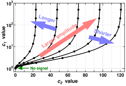
Figure 18: Theoretical predictions of the data point on a $c_{2}$-$c_{1}$ plot for given waveform parameters ($\alpha$ and $\beta_{2}$). The loci corresponds to the $\beta_{2}$ parameter of $\beta_{2}=122.21\times(0.2,0.4,0.6,0.8,1)$. The locus for a waveform with a large $\beta_{2}$ value (with a short time scale) appears on the right side of the plot.

From the calculations described above, we can estimate the expected values as $E(c_{1})$ and $E(c_{2})$ when the waveform and amplitude are given. Figure 18 shows the expected points for given waveforms in the $c_{2}$-$c_{1}$ plane; each curve is plotted by sweeping the power $\alpha$. When $\alpha$ is small, the ($c_{2}$, $c_{1}$) point is around (0, 1) independently of the waveform ($\beta_{2}$). (Here, we assume $M\gg 1$.) On the other hand, the position has a strong dependence on the $\beta_{2}$ parameter for large $\alpha$: $c_{2}\rightarrow\beta_{2}-1$, for $\alpha\gg 1$. Since signals with different time scales have different $\beta_{2}$ values, they appear along different loci.

Since the average time, $\Delta T$, is finite, and since the data contains the Gaussian noise components, the ($c_{2}$, $c_{1}$) data points have a distribution around the predicted curve shown in Fig. 18. With an approximation that $\Delta T$ (or data point number $N$) is sufficiently large, the ($c_{2}$, $c_{1}$) points for given $\alpha$ and $\beta_{2}$ have a two-dimensional Gaussian distribution, determined by the expected values ($E(c_{1})$ and $E(c_{2})$), the variances ($\mu_{2}(c_{1})$ and $\mu_{2}(c_{2})$), and the covariance $\mu_{11}(c_{1},c_{2})$. We define the distance between a reference point, which is calculated by a gravitational waveform (a reference waveform), and a data point by

$$D^{2} = {1\over V}\left\{{\mu_{2}(c_{2})\Delta c_{1}^{2}}\right.$$ (21)

$$\left.{-2\mu_{11}(c_{1},c_{2})\Delta c_{1}\Delta c_{2}+\mu_{2}(c_{1})\Delta c_{2}^{2}}\right\},$$

where $\Delta c_{1}$, $\Delta c_{2}$, and $V$ are defined by $\Delta c_{1}=c_{1}-E(c_{1})$, $\Delta c_{2}=c_{2}-E(c_{2})$, and $V=\mu_{2}(c_{1})\mu_{2}(c_{2})-\mu_{11}(c_{1},c_{2})$, respectively (Fig. 8). This distance, which is normalized by the variances and covariance, represents how similar these points are; if $D$ is small, the data point has a similar amplitude and a time scale as that of the reference point. Here, the minimum distance ($D_{\rm min}$) for various amplitudes ($\alpha$) is the similarity of the time scales of the data point and the reference waveform. Thus, we use $D_{\rm min}$ to distinguish fakes from the true GW signals. If the data points have a two-dimensional Gaussian distribution around their mean point, and if the variances and covariance are sufficiently smaller than the curvature of the locus, the minimal distance ($D_{\rm min}$) approximately obeys an exponential distribution,

$$P(D_{\rm min})\propto e^{-D_{\rm min}^{2}/2}.$$ (22)

For a practical implementation of the veto scheme, we should consider the acceptability of multiple reference waveforms and a reduction of the computational load. Thus, we adopted a conservative way for the veto analysis; we reject only the events with longer time scales than the longest one in the reference waveforms (Fig. 9). We use one waveforms with the smallest $\beta_{2}$ value, i.e. with the longest time scale, as the reference waveform, and set $D_{\rm min}=0$ if the data point is on the right side of the reference locus in the $c_{1}$-$c_{2}$ plot. In addition, we prepare a map of $D_{\rm min}$ in the $c_{1}$-$c_{2}$ plane before the data analysis, so as to reduce the computational load during the data analysis.

References

- (1) K. S. Thorne, in: Three hundred years of gravitation, eds: S. Hawking and W. Israel (Cambridge University Press) p. 330-458 (1987).
- (2) A. Abramovici et al., Science 256 325 (1992).
- (3) The VIRGO collaboration, VIRGO Final Design Report VIR-TRE-1000-13 (1997), C. Bradaschia, et al., Nucl. Instrum. Meth. A 289 518 (1990).
- (4) K. Danzmann et al., Proposal for a 600m Laser-Interferometric Gravitational Wave Antenna (Max-Planck-Institut für Quantenoptik Report) 190 (1994).
- (5) K. Tsubono, Gravitational Wave Experiments, eds: E. Coccia, G. Pizzella, and F. Ronga (World Scientific) p. 112 (1995), K. Kuroda et al., Gravitational Waves: Sources and Detectors, eds: I. Ciufolini and F. Fidecaro (World Scientific) p. 100 (1997).
- (6) M. Ando et al., Phys. Rev. Lett. 86 3950 (2001).
- (7) K. S. Thorne, Rev. Mod. Phys. 52 285 (1980).
- (8) B. F. Schutz, Class. Quantum Grav. 16 A131 (1999).
- (9) B. Allen et al., Phys. Rev. Lett. 83 1498 (1999).
- (10) H. Tagoshi et al., Phys. Rev. D 63 062001 (2001).
- (11) T. M. Niebauer et al., Phys. Rev. D 47 3106 (1993), K. Soida et al., Class. Quantum Grav. 20 S645 (2003).
- (12) B. Abbott et al., Phys. Rev. D 69 082004 (2004).
- (13) H. Dimmelmeier , J. A. Font, and E. Müller, Astron. Astrophys. 393 523 (2002).
- (14) T. Zwerger and E. Müller, Astron. Astrophys. 317 L79 (1997), E. Müller, M. Rampp, R. Buras, H. Janka, and D. Shoemaker, Astrophysical Journal 603 221 (2004).
- (15) C. D. Ott, A. Burrows, E. Livne, and R. Walder Ap. J. 600 834 (2004), T. Harada, H. Iguchi, and M. Shibata, Phys. Rev. D 68 024002 (2003), K. Kotake, S. Yamada, and K. Sato, Phys. Rev. D 68 044023 (2003).
- (16) W. G. Anderson et al., Phys. Rev. D 63 042003 (2001), W. G. Anderson et al., Phys. Rev. D 60 102001 (1999), A. Viceré, Phys. Rev. D 66 062002 (2002).
- (17) S. S. Mohanty, Phys. Rev. D 61 122002 (2000).
- (18) T. Pradier et al., Phys. Rev. D 63 042002 (2001), N. Arnaud et al., Phys. Rev. D 67 062004 (2003).
- (19) N. Arnaud et al., Phys. Rev. D 59 082002 (1999).
- (20) B. Allen, Phys. Rev. D accepted, gr-qc/0405045.
- (21) D. Nicholson et al., Phys. Lett. A 218 175 (1996).
- (22) H. Takahashi et al., Phys. Rev. D 70 042003 (2004), N. Arnaud et al., Phys. Rev. D 68 102001 (2003).
- (23) P. Astone et al., Phys. Rev. D 59 122001 (1999), Z. Allen et al., Phys. Rev. Lett. 85 5046 (2000), P. Astone et al., Class. Quantum Grav. 11 2093 (1994).
- (24) L. Cadonati and E. Katsavounidis, Class. Quantum Grav. 20 S633 (2003), K. Kotter et al., Class. Quantum Grav. 20 S895 (2003).
- (25) S. D. Mohanty and S. Mukherjee, Class. Quantum Grav. 19 1471 (2002).
- (26) M. Ando et al., Class. Quantum Grav. 20 S697 (2003).
- (27) R. Takahashi et al., Class. Quantum Grav. 21 S403 (2004), M. Ando, Class. Quantum Grav. 19 1409 (2002).
- (28) M. Ando et al., Class. Quantum Grav. 21 S735 (2004).
- (29) B. Abbott et al., Phys. Rev. D 69 102001 (2004).
- (30) P. Astone et al., Phys. Rev. D 68 022001 (2003).
- (31) S. Telada et al., in: Gravitational Wave detection II, eds.: S. Kawamura, N. Mio (Universal Academy Press) pp. 129-136 (2000), N. Kanda and the TAMA Collaboration, Int. J. Mod. Phys. D 9 233 (2000),
- (32) D. Tatsumi et al., in: Gravitational Wave detection II, eds.: S. Kawamura, N. Mio, Universal Academy Press (2000) pp. 113-121.
- (33) R. Wainscoat, M. Cohen, K. Volk, H. Walker, and D. Schwartz, Ap. J. S. 83 111 (1992) and the references therein.
- (34) J. Larsen and R. Humphreys, Astronomical Journal 125 1958 (2003).
- (35) P. J. Sutton et al., Class. Quantum Grav. 21 S1801 (2004).
- (36) K. Kuroda et al., Int. J. Mod. Phys. D 8 557-579 (1999), K. Kuroda et al., Class. Quantum Grav. 20 S871 (2003).
- (37) LIGO Scientific Collaboration, ed: P. Fritschel, LIGO Technical Note T010075, A. Weinstein, Class. Quantum Grav. 19 1575 (2002).
- (38) H. Cramer, Mathematical methods of statistics (Princeton University Press, 1946).
- (39) W. Press et al., Numerical Recipes in C (Cambridge University Press, 1988).