Probing anisotropies of gravitational-wave backgrounds
with a space-based interferometer:
Geometric properties of antenna patterns and their angular power

Abstract

We discuss the sensitivity to anisotropies of stochastic gravitational-wave backgrounds (GWBs) observed via space-based interferometer. In addition to the unresolved galactic binaries as the most promising GWB source of the planned Laser Interferometer Space Antenna (LISA), the extragalactic sources for GWBs might be detected in the future space missions. The anisotropies of the GWBs thus play a crucial role to discriminate various components of the GWBs. We study general features of antenna pattern sensitivity to the anisotropies of GWBs beyond the low-frequency approximation. We show that the sensitivity of space-based interferometer to GWBs is severely restricted by the data combinations and the symmetries of the detector configuration. The spherical harmonic analysis of the antenna pattern functions reveals that the angular power of the detector response increases with frequency and the detectable multipole moments with effective sensitivity $h_{\rm eff}\sim 10^{-20}$Hz^-1/2 may reach $\ell\sim 8$–$10$ at $f\sim f_{*}=10$ mHz in the case of the single LISA detector. However, the cross correlation of optimal interferometric variables is blind to the monopole ($\ell=0$) intensity anisotropy, and also to the dipole ($\ell=1$) in some case, irrespective of the frequency band. Besides, all the self-correlated signals are shown to be blind to the odd multipole moments ($\ell=\mathrm{odd}$), independently of the frequency band.

I Introduction

Space-based gravitational wave detectors retain many possibilities of providing access to new gravitational-wave sources that are not covered by ground-based gravitational-wave detectors. The Laser Interferometer Space Antenna (LISA) is such a planned gravitational-wave observatory aimed at detecting and studying low-frequency gravitational waves in the band $0.1$ mHz $\sim$ $0.1$Hz. The constellation of the LISA and the next generation detectors, e.g. DECIGO/BBO Seto et al. (2001); Takahashi and Nakamura (2003); BBO (2003), will consist of three spacecrafts keeping a triangle configuration.

Compared to ground-based detectors, a space-based gravitational-wave detector is characterized by many different features. For instance, the LISA introduces complications unknown to ground-based detectors, such as the complex signal and noise transfer functions. The complications block the analytical characterization of the detector Vallisneri (2004); Cor (2003); Cornish and Rubbo (2003); Merkowitz (2003); Merkowitz et al. (2004), and in particular, the response of an interferometer becomes complicated for gravitational waves shorter than the arm length of the detector. Only in the low-frequency limit, the response of the LISA detector is very simplified. The three arms of the LISA function like a pair of two-arm detectors, and it is well known that the pair is equivalent in the low frequency limit to two $90^{\circ}$ interferometers which are rotated by $\pi/4$ with respect to each other (e.g. Cutler (1998)).

An important ingredient of a space-based detector is analysis of time-delayed combinations of data streams, which provide laser-noise-free interferometric variable. The technique to synthesize data streams is known as time delay interferometry (TDI) Tinto and Armstrong (1999); Armstrong et al. (1999); Dhurandhar et al. (2002); Prince et al. (2002). Several TDI signals, such as Michelson-like and Sagnac-like signals which are free from the laser frequency noise, will have different responses to secondary phase noise sources and to incoming gravitational waves. Starting with the original TDI observables for stationary-array combinations, the TDI observables have been developed until recently (see Krolak et al. (2004) and references therein).

Space-based gravitational-wave detectors could be the most suitable devices to study and search for stochastic gravitational-wave signals. Examples of stochastic gravitational waves are those produced by large populations of Galactic Hils et al. (1990); Bender and Hils (1997); Nelemans et al. (2001) and extra-galactic binaries Kosenko and Postnov (1998); Schneider et al. (2001); Farmer and Phinney (2003) and a primordial gravitational-wave background produced by several cosmological mechanisms (see Maggiore (2000) for a review). Stochastic gravitational waves are expected to be anisotropic, and an important issue is to identify unambiguously the anisotropy to get insights into the origin and underlying physics of them.

A method to explore an anisotropy of gravitational-wave background has been recently proposed based on the time modulation of the single data stream Giampieri and Polnarev (1997a, b); Cornish (2001, 2002a); Ungarelli and Vecchio (2001) and/or the two data streams Cornish (2001); Seto and Cooray (2004); Allen and Ottewill (1997), which allow us to extract the individual coefficients of multipole moments related to a distribution of gravitational waves on the sky. Hence, provided all the coefficients of multipole moments observationally, one can, in principle, make the sky map of the gravitational-wave backgrounds Cornish (2001, 2002a). It was demonstrated in the low frequency limit that the LISA is blind to the whole set of odd multipole moments and sensitive only to monopole ($\ell=0$), quadrupole ($\ell=2$) and octupole ($\ell=4$) anisotropy Ungarelli and Vecchio (2001); Cornish (2001). Actually, the multipole moments $\ell=2,4$ and their $m$ th harmonics of the galactic distribution of binaries would be observable with sufficiently high signal-to-noise ratios, except for some multipole harmonics Seto and Cooray (2004). The restricted sensitivity to the multipole moments is an immediate outcome of the low-frequency approximation, but what is the underlying physics that determines the limitation? As discussed in this paper, it is intimately associated with the geometric properties of the spacecraft configuration.

So far most of the works aimed at probing the anisotropy of gravitational-wave background by means of space-based interferometers have been restricted to the low-frequency approximation. One reason is that a confusion gravitational-wave background formed by the superposition of many Galactic binaries comes in the low-frequency band of the LISA as the dominant source Hils et al. (1990). However there are many expected sources of gravitational-wave backgrounds that spread outside the low-frequency region Kosenko and Postnov (1998); Schneider et al. (2001); Farmer and Phinney (2003); Schneider et al. (2000); Enoki et al. (2004). Thus it is an interesting problem to create maps of the gravitational-wave background in a very wide range of frequency. For that purpose we need to know the general response and properties of space-based interferometer over a wide range of frequency.

In this paper we are interesting in general features of response function for space-based detectors. The sensitivity of space-based detectors to multipole moments of a gravitational-wave distribution is in general restricted by symmetries of a response function independently of frequency. For example, symmetries of a response function tell us that a self-correlated data is blind to the odd multipole moments of anisotropy irrespective of frequency band (Sec. IV.3). Other interesting features independent of frequency can be also derived based on symmetries of a detector’s response and geometric configuration of the spacecrafts.

The paper is organized as follows. After briefly reviewing the detection method of an anisotropy by the correlation analysis in the next section, detector response functions for space-based interferometers are given in Sec. III. In Sec. IV, we develop spherical harmonic analysis of antenna pattern functions and derive various fundamental properties of multipole moments. Based on those fundamental properties, in Sec. V, we examine the directional sensitivity of space interferometer. Angular power and effective sensitivity curves are discussed there, specifically focusing on the LISA detector. Section VI concludes the paper with a brief summary. Below the speed of light is set equal to unity ($c=1$).

II detection of anisotropy through the correlation analysis

We begin by discussing how one can prove the anisotropy of gravitational-wave background based on the correlation analysis. A stochastic background of gravitational waves can be expressed as a random superposition of plane waves propagating along $\mathbf{\Omega}=-\textbf{n}$ direction with surfaces of constant phase $\xi(\bf{x})=t+{\bf n\cdot x}$. Then the metric perturbation in transverse-traceless gauge h is expressed as:

$$\textbf{h}(t,\textbf{x})=\sum_{A=+,\times}\int_{-\infty}^{\infty}df\int d\mathbf{\Omega}\,\,e^{i\,2\pi\,f\xi}\widetilde{h}_{A}(f,\mathbf{\Omega})\,\,{\bf{e}}^{A}(\mathbf{\Omega}),$$ (1)

where $\int d\mathbf{\Omega}$ denotes an integral over the sphere and $\tilde{h}_{A}(-f)=\tilde{h}^{*}_{A}{(f)}$ are the Fourier amplitudes of the gravitational waves for each polarization mode. The Fourier amplitudes $h_{A}$ is assumed to be characterized by the Gaussian random process:

$$\left\langle\widetilde{h}_{A}(f,{\bf{\Omega}})\right\rangle = 0,$$ (2)

$$\left\langle\widetilde{h}_{A}^{*}(f,{\bf{\Omega}}){{\widetilde{h}}_{A^{\prime}}}(f^{\prime},{\bf{\Omega}}^{\prime})\right\rangle = \frac{1}{2}\delta(f-f^{\prime})\frac{\delta^{2}({\bf{\Omega}},{\bf{\Omega}}^{\prime})}{4\pi}\delta_{AA^{\prime}}S_{h}(|f|,\,\mathbf{\Omega}),$$ (3)

where $S_{h}(|f|,\,{\bf\Omega})$ is the power spectral density of gravitational waves. The polarization tensors ${\bf{e}}^{A}(\bf{\Omega})$ appearing in equation (1) may be explicitly given as follows:

$${\bf e}^{+}({\bf{\Omega}})={\bf u}\otimes{\bf u}-{\bf v}\otimes{\bf v},\quad{\bf e}^{\times}({\bf{\Omega}})={\bf u}\otimes{\bf v}+{\bf v}\otimes{\bf u},\,\,$$ (4)

where the unit vectors ${\bf u}$, ${\bf v}$ are expressed in an ecliptic coordinate as:

$${\bf u} = \cos\theta_{E}\cos\phi_{E}{\bf x}+\cos\theta_{E}\sin\phi_{E}{\bf y}-\sin\theta_{E}{\bf z},$$ (5)

$${\bf v} = \sin\phi_{E}{\bf x}-\cos\phi_{E}{\bf y},$$ (6)

$${\bf n} = \sin\theta_{E}\cos\phi_{E}{\bf x}+\sin\theta_{E}\sin\phi_{E}{\bf y}+\cos\theta_{E}{\bf z}=-{\bf\Omega}.$$ (7)

The detection of a gravitational-wave background is achieved through the correlation analysis of two data streams. The output signal for the detector $I$ denoted by $s_{I}(t)$ is described by a sum of the gravitational-wave signal $h_{I}(t)$ and the detector noise $n_{I}(t)$:

$$s_{I}(t)=h_{I}(t)+n_{I}(t).$$

We assume that the noise $n_{I}(t)$ is treated as a Gaussian random process with zero mean and spectral density $S_{\rm n}(f)$:

$$\left\langle\widetilde{n}_{I}(f)\right\rangle = 0,$$

$$\left\langle\widetilde{n}_{I}^{*}(f){{\widetilde{n}}_{J}}(f^{\prime})\right\rangle = \frac{1}{2}\delta(f-f^{\prime})\,\delta_{IJ}\,\,S_{\rm n}(|f|).$$

Here, we further assume that the noise correlation between the two independent detectors is neglected .

On the other hand, in addition to the information of a gravitational-wave background, the output signal $h_{I}(t)$ contains the time variation of the detector response caused by the detector motion. For example, the rotation of the Earth sweeps the ground-based interferometer across the sky. As for the space interferometer, LISA, the antenna pattern sweeps over the sky as the LISA constellation orbits around the sun with period of one sidereal year. These effects induce the signal modulation, which can be used to extract the information of anisotropy of gravitational-wave backgrounds.

According to Ref.Allen and Ottewill (1997), we introduce two time-scales, $\Delta T$ and $T_{0}$: the light travel time $\Delta T$ between the two detectors (space crafts) and the period of the detector motion $T_{0}$. Since $\Delta T\ll T_{0}$, it is possible to choose the averaging time scale $\tau$ as $\Delta T\ll\tau\ll T_{0}$ appropriately. Then, one can safely employ the correlation analysis between two detectors as a function of time averaged over the period $\tau$. Keeping this situation in mind, the output signal $h_{I}(t)$ may be written as

$$h_{I}(t)=\sum_{A=+,\times}\int_{-\infty}^{+\infty}df\int d\mathbf{\Omega}\,\,\textbf{D}_{I}(\mathbf{\Omega},f;t)\,\textbf{:}~{}\textbf{e}^{A}(\mathbf{\Omega})\,\,\widetilde{h}_{A}(f,\mathbf{\Omega})\,\,e^{i2\pi f\,\xi(x_{I})},$$ (8)

where the colon denotes the double contraction, i.e., $\textbf{D:\,e}=D_{ij}e^{ij}$ Cornish and Larson (2001). The quantity D is detector’s response function, whose explicit expression will be presented in next section. Note that the response function depends on time due to the detector motion.

Provided the two output data sets, the correlation analysis is examined depending on the strategy of data analysis, i.e., self-correlation analysis only using the single data stream or cross-correlation analysis using the two independent data stream:

$$C(t) \equiv \left\langle s_{I}(t)s_{J}(t)\right\rangle=\left\langle h_{I}(t)h_{J}(t)\right\rangle+\left\langle n_{I}(t)n_{J}(t)\right\rangle$$

$$= \int^{\infty}_{-\infty}\frac{df}{2}\int\frac{d\mathbf{\Omega}}{4\pi}S_{h}(|f|,\mathbf{\Omega})~{}\mathcal{F}_{IJ}^{E}(f,\mathbf{\Omega};\,t)+\delta_{IJ}\int^{\infty}_{-\infty}\frac{df}{2}S_{n}(|f|),$$

where $\mathcal{F}^{E}_{IJ}$ is the antenna pattern function defined in an ecliptic coordinate, which is expressed in terms of detector’s response function and an optimal filter:

$$\mathcal{F}^{E}_{IJ}(f,\mathbf{\Omega};\,t)=e^{i\,2\pi f{\bf\Omega\cdot}(\textbf{x}_{I}-\textbf{x}_{J})/L}\sum_{A=+,\times}F_{I}^{A*}(\mathbf{\Omega},f;\,t)F_{J}^{A}(\mathbf{\Omega},f;\,t)\,\widetilde{Q}(f)\,$$ (9)

$$F_{I}^{A}(\mathbf{\Omega},f;\,t)={\bf D}_{I}(\mathbf{\Omega},f;\,t)\,\textbf{:}\,\textbf{e}^{A}(\mathbf{\Omega})$$ (10)

with $\widetilde{Q}(f)$ being the Fourier transform of the optimal filter. Note that the phase factor $e^{i\,2\pi\,f\,\mathbf{\Omega}{\cdot}(\textbf{x}_{I}-\textbf{x}_{J})/L}$ arises due to the differences between the arrival time of the signal at each detector. The above expression implies that the time series data $C(t)$ as observable is given by the all-sky integral of the spectral density $S_{h}$, or luminosity distribution of gravitational waves convolving with the antenna pattern function. To see this more clearly, for the moment, we neglect the noise contribution and set the optimal filter as $\tilde{Q}(f)=1$. Keeping the assumption $\Delta T\ll t\ll T_{0}$, the detector output $C(t)$ is written as

$$C(t) = \int_{-\infty}^{\infty}\frac{df}{2}\,\,\widetilde{C}(t,f)$$ (11)

$$= \int_{-\infty}^{\infty}\frac{df}{2}\int\frac{d\mathbf{\Omega}}{4\pi}~{}{S}_{h}(|f|,\mathbf{\Omega})\,\mathcal{F}^{E}_{IJ}(f,t,\mathbf{\Omega}).$$ (12)

We then decompose the antenna pattern function $\mathcal{F}_{IJ}^{E}$ and the luminosity distribution into spherical harmonics in an ecliptic coordinate, i.e., sky-fixed frame. We have

$$S_{h}(|f|,\,\mathbf{\Omega})=\sum_{\ell m}[p^{E}_{\ell m}(f)]^{*}\,\,Y_{\ell m}^{*}(\mathbf{\Omega}),\quad\mathcal{F}^{E}_{IJ}(f,\,\mathbf{\Omega};\,t)=\sum_{\ell m}a_{\ell m}^{E}(f,t)\,\,Y_{\ell m}(\mathbf{\Omega}).$$ (13)

Substituting (13) into (12) becomes

$$\widetilde{C}(t,f)=\frac{1}{4\pi}\,\sum_{\ell m}\,\,\left[p^{E}_{\ell m}(f)\right]^{*}a^{E}_{\ell m}(f,\,t).$$ (14)

Note that the time dependent multipole coefficient $a^{E}_{\ell m}$ appears due to the detector motion, which can be eliminated by further employing the harmonic expansion in detector’s rest frame $(\theta,\phi)$. We denote the multipole coefficients of the antenna pattern in detector’s rest frame by $a_{\ell m}$ (see Eq.[40]). The transformation between the detector rest frame and the sky-fixed frame is described by a rotation matrix by the Euler angles $(\psi,\vartheta,\varphi)$, whose explicit relation is expressed in terms of the Wigner $D$ matrices Allen and Ottewill (1997); Cornish (2002a); Edmonds (1957):

$$a^{E}_{\ell m}(f,t)=\sum_{n=-\ell}^{\ell}e^{-i\,n\,\psi}\,d^{\ell}_{nm}(\vartheta)\,e^{-i\,m\,\varphi}\,\,a_{\ell n}(f).$$ (15)

Here the Euler rotation is defined to perform a sequence of rotation, starting with a rotation by $\psi$ about the original $z$ axis, followed by rotation by $\vartheta$ about the original $y$ axis, and ending with a rotation by $\varphi$ about the original $z$ axis. Note that the Euler rotation conserves the multipole moment $\ell$, but mixes $m$-th harmonics.

For illustration, let us envisage the orbital motion of the LISA constellation. The LISA orbital motion can be expressed by $\psi=-\omega t$, $\vartheta=-\pi/3$, $\varphi=\omega t$, where $\omega=2\pi/T_{0}$ is LISA’s orbital frequency ($T_{0}=1$ sidereal year). Since the antenna pattern function is periodic in time due to the orbital motion, one can naturally perform the Fourier transformation of the detector output by Giampieri and Polnarev (1997a); Cornish (2001):

$$\tilde{C}_{k}(f)=\frac{1}{T_{0}}\int^{T_{0}}_{0}dt~{}e^{-ik\omega t}\,\,\tilde{C}(t,f).$$

Using the relation (15), we finally obtain:

$$\tilde{C}_{k}(f)=\frac{1}{4\pi}\,\,\sum_{\ell=0}^{\infty}\sum_{m=-\ell}^{\ell-k}[p_{\ell m}^{E}(f)]^{*}\,\,d^{\ell}_{(m+k),m}\left(\vartheta\right)\,a_{\ell,(m+k)}(f),$$ (16)

for $k\geq 0$. The above equation shows how the detector output depends on the multipole coefficients $a_{\ell m}$ in detector’s rest frame for a given luminosity distribution of a gravitational-wave background, $p_{\ell m}^{E}(f)$. Given the output data $\tilde{C}_{k}(f)$ experimentally, the task is to solve the linear system (16) with respect to $p_{\ell m}^{E}(f)$ if we know the antenna pattern function. As discussed by Cornish Cornish (2001), this deconvolution problem is typically either over-constrained or under-constrained depending on the antenna pattern. In this sense, the understanding of the general properties of antenna pattern functions is primarily important and would shed light on the deconvolution problem. It might be further helpful to characterize the directional sensitivity to the sky map of the gravitational-wave background. The detailed investigation for the spherical harmonic analysis of antenna pattern will be presented in Sec. IV. Before developing the analysis, we briefly review the detector response functions for space interferometers.

III Detector response function for space interferometer

In this section, according to the treatment based on the coordinate-free approach in Ref. Cornish and Rubbo (2003); Cornish (2002b), we derive various types of detector response functions for space interferometer, which will be used to analyze the sensitivity to an anisotropy of gravitational-wave background.

III.1 One-arm detector tensor

Following the Doppler tracking calculations described in Ref. Cornish and Larson (2001), the optical-path length between spacecraft $i$ and spacecraft $j$ is formally written as

$$\ell_{ij}(t_{i})=\int^{j}_{i}\sqrt{g_{\mu\nu}dx^{\mu}dx^{\nu}},$$ (17)

where $g_{\mu\nu}$ is spacetime metric. According to Ref. Cornish and Rubbo (2003), the optical-path variation in presence of the gravitational waves is given by

$$\delta\ell_{ij}(t_{i})=\ell_{ij}(t_{i})\int^{\infty}_{-\infty}df\,\,\int\,d\mathbf{\Omega}\,\,\,\textbf{D}(f,t_{i},{\bf n})\textbf{:}\tilde{\textbf{h}}(f,\,\mathbf{\Omega})e^{i\,2\pi\,f(t_{i}+{\bf n}\cdot\textbf{x}_{i})},$$ (18)

where the one-arm detector tensor D and the transfer function $\mathcal{T}$ are

$$\textbf{D}(f,t_{i},\textbf{n}) = \frac{1}{2}[\textbf{r}_{ij}(t_{i})\otimes\textbf{r}_{ij}(t_{i})]\mathcal{T}(w,t_{i},\textbf{n}),$$ (19)

$$\mathcal{T}(f,t_{i},\textbf{n}) = {\mathrm{sinc}}\left[\frac{f}{2f_{ij}}[1+\textbf{n}\cdot\textbf{r}_{ij}(t_{i})]\right]\exp\left[i\frac{f}{2f_{ij}}[1+\textbf{n}\cdot\textbf{r}_{ij}(t_{i})]\right],$$ (20)

where $\textbf{r}_{ij}(t_{i})$ is the unit vector pointing from the space craft $i$ at the time of emission $t_{i}$ to the space craft $j$ at the time of reception $t_{j}$, i.e., $\textbf{r}_{ij}(t_{i})=\{{\bf x}_{j}(t_{j})-{\bf x}_{i}(t_{i})\}/l_{ij}(t_{i})$. The function ${\mathrm{sinc}}(x)$ is defined by ${\mathrm{sinc}}(x)=\sin x/x$ and the variable $f_{ij}=[2\pi\ell_{ij}(t_{j})]^{-1}$ means the characteristic transfer frequency.

III.2 Detector response function

The calculation of the one-arm detector tensor can be applied to derive the response function for a space interferometer via Doppler tracking method. The constellation of the planned space interferometer, LISA and also the next generation detectors DECIGO/BBO constitutes three space crafts and each of them is separated in an equal arm length (Fig. 1). Note cautiously that the detector arm length varies in time, mainly due to the intrinsic variation by the Keplerian motion of three spacecrafts and the tidal variation caused by the gravitational force of Solar System planets Bender and et. al., (1998); Rubbo et al. (2004). The caveats concerning these effects have been already mentioned Cornish and Hellings (2003) and their influences were recently investigated. As long as the low-frequency gravitational waves with frequencies comparable or lower than the characteristic frequency $f_{ij}$ are concerned Cornish and Rubbo (2003); Rubbo et al. (2004); Vecchio and Wickham (2004), the so-called rigid adiabatic approximation Rubbo et al. (2004), in which the three space crafts rigidly orbit around the sun under keeping their configuration, really works.

Keeping these remarks in mind, we adopt the rigid adiabatic approximation to give an analytic expression for response functions. For the sake of the brevity, we work with the static and the equal-arm limit of the detector response. In this case, one writes $L=l_{ij}$ and $f_{*}\equiv f_{ij}=1/(2\pi L)$. Thus, the interferometric signals combining with the six data streams can be generally expressed as function of

$$\hat{f}\equiv\frac{f}{f_{*}}.$$ (21)

Specifically, for LISA detector, the arm length is $L=5\times 10^{6}$km, yielding $f_{*}\simeq 10$mHz.

Based on the configuration in Fig. 1, a signal of Michelson interferometers extracted from the space craft $1$ is Cornish and Rubbo (2003); Cornish (2002b):

$$h_{\scriptscriptstyle\rm M_{1}}(t) = \frac{1}{2L}\Bigl{[}\delta\ell_{12}(t-2L)+\delta\ell_{21}(t-L)-\delta\ell_{13}(t-2L)-\delta\ell_{31}(t-L)\Bigr{]}$$ (22)

$$= \int^{\infty}_{-\infty}df\,\,\int d\mathbf{\Omega}\,\,\textbf{D}_{\scriptscriptstyle\rm M_{1}}(\mathbf{\Omega},f)\textbf{:}\widetilde{\textbf{h}}(f,\mathbf{\Omega})\,\,e^{i\,2\pi\,f\xi(x_{1})},$$ (23)

where $\textbf{D}_{\scriptscriptstyle\rm M_{1}}(\mathbf{\Omega},\,f)$ is the detector tensor. The explicit form of the detector tensor is given by

$${\bf D}_{\scriptscriptstyle\rm M_{1}}(\mathbf{\Omega},f) = \frac{1}{2}\left\{({\bf a}\otimes{\bf a})\,{\cal T}_{\scriptscriptstyle\rm M}({\bf a}\cdot{\bf\Omega},f)-({\bf c}\otimes{\bf c})\,{\cal T}_{\scriptscriptstyle\rm M}(-{\bf c}\cdot{\bf\Omega},f)\right\}~{}~{};$$ (24)

$${\cal T}_{\scriptscriptstyle\rm M}({\bf u}\cdot{\bf\Omega},f) = e^{-i{\hat{f}}}\left\{{\mathrm{sinc}}\left(\frac{{\hat{f}}(1-{\bf u}\cdot{\bf\Omega})}{2}\right)e^{-\frac{i}{2}{\hat{f}}(1+{\bf u}\cdot{\bf\Omega})}+{\mathrm{sinc}}\left(\frac{{\hat{f}}(1+{\bf u}\cdot{\bf\Omega})}{2}\right)e^{-\frac{i}{2}{\hat{f}}(-1+{\bf u}\cdot{\bf\Omega})}\right\}.$$ (25)

The directional unit vectors for the three space crafts are denoted by $\mathbf{a},\mathbf{b},\mathbf{c}$ (Fig. 1). Note that the above expression possesses the symmetry, i.e., ${\bf D}_{\scriptscriptstyle\rm M}(\mathbf{\Omega},-f)={\bf D}_{\scriptscriptstyle\rm M}(\mathbf{\Omega},f)^{*}$.

Unfortunately, the simple Michelson interferometry with unequal armlengths does not cancel the laser frequency noise, which is thought to be one of the most dominant sources in the instrumental noises. Thus, the Michelson signal might not be a viable interferometric variable. Instead, a number of so-called TDI variables that cancel the laser frequency noise even when the armlengths are unequal have been proposed (Armstrong et al., 1999). These signals are built by combining time-delayed Michelson signals so as to reduce the overall laser frequency noise down to a level of other noises. A particular example of a TDI variable is the X signal:

$$h_{\scriptscriptstyle\rm X_{1}}(t) = \frac{1}{4L}\Bigl{[}\delta\ell_{12}(t-2L)-\delta\ell_{12}(t-4L)+\delta\ell_{21}(t-L)-\delta\ell_{21}(t-3L)$$ (26)

$$-\delta\ell_{13}(t-2L)+\delta\ell_{13}(t-4L)-\delta\ell_{31}(t-L)+\delta\ell_{31}(t-3L)\Bigr{]}.$$

This signal is expressed by a superposition of the Michelson signal, $s_{\scriptscriptstyle\rm X_{1}}(t)=\frac{1}{2}[s_{1}^{\scriptscriptstyle\rm M}(t)-s_{1}^{\scriptscriptstyle\rm M}(t-2L)]$. Thus, the detector tensor for the interferometer variable is ${\bf D}_{\scriptscriptstyle\rm X}=\frac{1}{2}(1-e^{-2i\hat{f}}){\bf D}_{\scriptscriptstyle\rm M}$.

Other useful combination comes from comparing the phase of signals that are sent clockwise and counter-clockwise around the triangle. Such combination is named as Sagnac signal. The Sagnac signal extracted from the space craft $1$ is

$$h_{\scriptscriptstyle\rm S_{1}}(t) = \frac{1}{3L}\Big{[}\delta\ell_{13}(t-3L)+\delta\ell_{32}(t-2L)+\delta\ell_{21}(t-L)-\delta\ell_{12}(t-3L)-\delta\ell_{23}(t-2L)-\delta\ell_{31}(t-L)\Big{]}$$ (27)

$$= \int^{\infty}_{-\infty}df\,\,\int d\mathbf{\Omega}\,\,{\bf D}_{\scriptscriptstyle\rm S_{1}}({\bf\Omega},f)\,\textbf{:}\,\widetilde{\textbf{h}}(f,\,{\bf\Omega})\,\,e^{2\pi if\xi(x_{1})},$$ (28)

where the detector tensor ${\bf D}_{\scriptscriptstyle\rm S_{1}}$ is expressed as

$${\bf D}_{\scriptscriptstyle\rm S_{1}}({\bf\Omega},f) = \frac{1}{6}\left\{({\bf a}\otimes{\bf a}){\cal T}_{\rm a}(f)+({\bf b}\otimes{\bf b})\,{\cal T}_{\rm b}(f)\right.+\left.({\bf c}\otimes{\bf c})\,{\cal T}_{\rm c}(f)\right\}~{}~{};$$ (29)

$${\cal T}_{\rm a}(f) = e^{-3i{\hat{f}}/2}\left\{e^{-\frac{1}{2}i{\hat{f}}(-2+{\bf a}\cdot{\bf\Omega})}{\mathrm{sinc}}\left[\frac{{\hat{f}}}{2}\left(1+{\bf a}\cdot{\bf\Omega}\right)\right]-e^{-\frac{1}{2}i{\hat{f}}(2+{\bf a}\cdot{\bf\Omega})}{\mathrm{sinc}}\left[\frac{{\hat{f}}}{2}\left(1-{\bf a}\cdot{\bf\Omega}\right)\right]\right\},$$ (30)

$${\cal T}_{\rm b}(f) = e^{-\frac{1}{2}i{\hat{f}}(3+({\bf a}-{\bf c})\cdot{\bf\Omega})}\left\{{\mathrm{sinc}}\left[\frac{{\hat{f}}}{2}\left(1+{\bf b}\cdot{\bf\Omega}\right)\right]-{\mathrm{sinc}}\left[\frac{{\hat{f}}}{2}\left(1-{\bf b}\cdot{\bf\Omega}\right)\right]\right\},$$ (31)

$${\cal T}_{\rm c}(f) = e^{-\frac{3}{2}i{\hat{f}}}\left\{e^{-\frac{1}{2}i{\hat{f}}(2-{\bf c}\cdot{\bf\Omega})}{\mathrm{sinc}}\left[\frac{{\hat{f}}}{2}\left(1+{\bf c}\cdot{\bf\Omega}\right)\right]-e^{\frac{1}{2}i{\hat{f}}(2+{\bf c}\cdot{\bf\Omega})}{\mathrm{sinc}}\left[\frac{{\hat{f}}}{2}\left(1-{\bf c}\cdot{\bf\Omega}\right)\right]\right\}.$$ (32)

The three Sagnac signals extracted from the space crafts $1$, $2$ and $3$ are often quoted as $\alpha,\beta$, and $\gamma$ in the literature (e.g., Armstrong et al. (1999)). Combining these variables, a set of optimal data combinations free from the noise correlations is constructedPrince et al. (2002) (see also Krolak et al. (2004)):

$$h_{\rm A} = \frac{1}{\sqrt{2}}(h_{\scriptscriptstyle\rm S_{3}}-h_{\scriptscriptstyle\rm S_{1}}),$$ (33)

$$h_{\rm E} = \frac{1}{\sqrt{6}}(h_{\scriptscriptstyle\rm S_{1}}-2h_{\scriptscriptstyle\rm S_{2}}+h_{\scriptscriptstyle\rm S_{3}}),$$ (34)

$$h_{\rm T} = \frac{1}{\sqrt{3}}(h_{\scriptscriptstyle\rm S_{1}}+h_{\scriptscriptstyle\rm S_{2}}+h_{\scriptscriptstyle\rm S_{3}}).$$ (35)

It is worthwhile to note that in the low-frequency limit $\hat{f}\ll 1$, the detector tensor for the Michelson, the X and the Sagnac signal can be simply expressed as

$$i\,\hat{f}\,{\bf D}_{\scriptscriptstyle\rm M_{1}}={\bf D}_{\scriptscriptstyle\rm X_{1}}=\frac{3}{2}\,\,{\bf D}_{\scriptscriptstyle\rm S_{1}}=\frac{i\hat{f}}{2}\,\,({\bf a}\otimes{\bf a}-{\bf c}\otimes{\bf c})+\mathcal{O}(\hat{f}^{2})$$ (36)

Using the above expression, the detector tensors for optimal combinations A, E and T respectively become

$${\bf D}_{\scriptscriptstyle\rm A} = \frac{i\,\hat{f}}{3\sqrt{2}}\,\,\,\left(-{\bf a}\otimes{\bf a}-{\bf b}\otimes{\bf b}+2{\bf c}\otimes{\bf c}\right),$$

$${\bf D}_{\scriptscriptstyle\rm E} = \frac{i\,\hat{f}}{\sqrt{6}}\,\,\,\left({\bf a}\otimes{\bf a}-{\bf b}\otimes{\bf b}\right),$$ (37)

$${\bf D}_{\scriptscriptstyle\rm T} = \frac{\,\hat{f}^{2}}{12\sqrt{3}}\,\,\,\left\{({\bf a}\cdot{\bf\Omega})\,\,{\bf a}\otimes{\bf a}+({\bf b}\cdot{\bf\Omega})\,\,{\bf b}\otimes{\bf b}+({\bf c}\cdot{\bf\Omega})\,\,{\bf c}\otimes{\bf c}\right\}.$$

Note that the expression for detector tensor ${\bf D}_{\scriptscriptstyle\rm T}$ is higher order in $\hat{f}$, compared to the other detector tensors.

IV Spherical harmonic analysis of antenna pattern function

The correlation analysis described in Sec. II reveals that the signal modulation induced by detector motion can be used to extract the information of the anisotropy of the gravitational-wave background. One important remark is that the map-making capability crucially depends on the antenna pattern and/or the detector response function in detector’s rest frame. We then wish to clarify the relationship between the antenna pattern functions and the directional sensitivity to the gravitational-wave backgrounds. To investigate this issue, the spherical harmonic analysis of the antenna pattern function is employed and the general rules for multipole coefficients are derived based on the geometric properties of the antenna pattern.

IV.1 Angular power of antenna pattern function

Similar to the expression (10), antenna pattern function $\mathcal{F}$ defined in detector’s rest frame is written as

$$\mathcal{F}_{IJ}(f,\mathbf{\Omega})=e^{i\hat{f}{\bf\Omega\cdot}(\textbf{x}_{I}-\textbf{x}_{J})}\sum_{A=+,\times}F_{I}^{A*}(\mathbf{\Omega},f)F_{J}^{A}(\mathbf{\Omega},f)\,\widetilde{Q}(f)\,$$ (38)

$$F_{I}^{A}(\mathbf{\Omega},f)={\bf D}_{I}(\mathbf{\Omega},f)\textbf{:}\textbf{e}^{A}(\mathbf{\Omega}).$$ (39)

The multipole coefficient $a_{\ell m}$ for (39) is

$$a_{\ell m}(\hat{f})=\int_{0}^{\pi}d\theta\int_{0}^{2\pi}d\phi\sin\theta\,Y_{\ell m}^{*}(\theta,\phi)\,\mathcal{F}(\hat{f},\theta,\phi)$$ (40)

with $\hat{f}$ being defined in (21). We are primarily concerned with how the directional sensitivity depends on the choice of the interferometric variables. For this purpose, the optimal filter $\widetilde{Q}(f)$ appearing in the antenna pattern function (10) is ignored hereafter. Using the fact that the relations ${\mathcal{F}}^{*}(\hat{f},{\bf\Omega})={\mathcal{F}}(-\hat{f},{\bf\Omega})={\mathcal{F}}(\hat{f},-{\bf\Omega})$ always hold, one obtains

$$a_{\ell,m}(\hat{f},t)=(-1)^{m}a_{\ell,-m}^{*}(-\hat{f},t)=(-1)^{m+\ell}a_{\ell,-m}^{*}(\hat{f},t).$$ (41)

where we used $Y_{\ell-m}(\theta,\phi)=(-1)^{m}Y_{\ell m}^{*}(\theta,\phi)$.

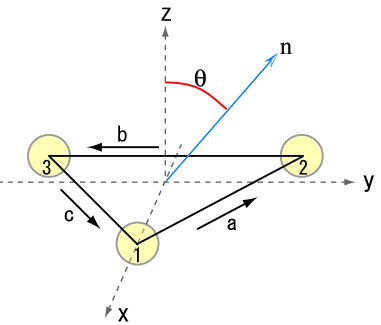
Figure 1: Configuration of the spacecraft constellation in detector’s rest frame.

Here and in what follows, we consider the detector configuration in a specific coordinate system shown in Fig. 1 to calculate the multipole coefficients. Unless otherwise stated, the unit vectors ${\bf a},{\bf b}$ and ${\bf c}$ are specifically chosen as:

$${\bf{a}}=-\frac{\sqrt{3}}{2}{\bf{x}}+\frac{1}{2}{\bf{y}},\quad{\bf{b}}=-{\bf{y}},\quad{\bf{c}}=\frac{\sqrt{3}}{2}{\bf{x}}+\frac{1}{2}{\bf{y}}.$$ (42)

While the explicit form of the multipole coefficients $a_{\ell m}$ depends on the coordinate system (42), a convenient quantity invariant under a Euler rotation of the coordinate system can be exploited:

$$\sigma_{\ell}^{2}(\hat{f})=\frac{1}{2\ell+1}\sum_{m=-\ell}^{\ell}|a_{\ell m}(\hat{f})|^{2},$$ (43)

which characterizes the contribution of $\ell$-th moment to the antenna pattern function. Thus, under the rigid adiabatic approximation, the angular power of the antenna pattern in the ecliptic frame is equivalent to that in detector’s rest frame:

$$\sum_{m}|a_{\ell m}(\hat{f})|^{2}=\sum_{m}|a_{\ell m}^{E}(\hat{f},t)|^{2}.$$ (44)

We use this coordinate invariant quantity to quantify the directional sensitivity of the antenna pattern.

IV.2 Low-frequency limit

Consider first the simplest case, $\hat{f}=f/f_{*}\ll 1$. In this case, only the $\ell=0$, $2$ and $4$ moments for antenna pattern function become non-vanishing. This is mostly general except for the fully symmetrized signals such as $T$-variable.

In the low-frequency limit, the detector response functions derived in previous section generally becomes of the form (see Eqs.[36][37]):

$${\bf D}\longrightarrow{\cal T}_{\rm a}({\bf a}\otimes{\bf a})+{\cal T}_{\rm b}({\bf b}\otimes{\bf b})+{\cal T}_{\rm c}({\bf c}\otimes{\bf c}),$$ (45)

except for the $T$-variable. While the factors ${\cal T}_{\rm a,b,c}$ may be written as functions of frequency, they do not depend on the directional angle ${\bf\Omega}$. Thus, the detector tensor ${\bf D}$ loses the directional dependence. This means that the directional dependence of the antenna pattern function $\mathcal{F}$ arises only through the polarization tensor, ${e}^{\rm A}({\bf\Omega})$. Since the polarization tensor is described by the quadrature of direction vectors ${\bf u}$ and ${\bf v}$ (Eq.[7]), the antenna pattern can be generally written as the forth order polynomials of $(\cos\theta,\sin\theta)$ and $(\cos\phi,\sin\phi)$. For example, the low-frequency limit of the self-correlated signal for Michelson and Sagnac interferometries extracted from the spacecraft $1$ is

$$\hat{f}^{2}\,\,{\mathcal{F}}_{\scriptscriptstyle\rm M_{1}M_{1}}=\frac{9}{4}{\mathcal{F}}_{\scriptscriptstyle\rm S_{1}S_{1}}~{}~{}\stackrel{{\scriptstyle\hat{f}\ll 1}}{{\longrightarrow}}~{}~{}\frac{3}{4}\left[\frac{1}{4}(3+\cos 4\phi)\cos^{2}\theta+(1+\cos^{4}\theta)\cos^{2}\phi\sin^{2}\phi\right]\hat{f}^{2}+{\mathcal{O}}(\hat{f}^{4}).$$ (46)

Applying the spherical harmonic expansion (40), non-vanishing components of the multipole coefficients become

$$a_{00}^{\scriptscriptstyle\rm M_{1}M_{1}}=\frac{3\sqrt{\pi}}{5},\quad a_{20}^{\scriptscriptstyle\rm M_{1}M_{1}}=\frac{6}{7}\sqrt{\frac{\pi}{5}},\quad a_{40}^{\scriptscriptstyle\rm M_{1}M_{1}}=\frac{\sqrt{\pi}}{70},\quad a_{4,\pm 4}^{\scriptscriptstyle\rm M_{1}M_{1}}=-\frac{1}{2}\sqrt{\frac{\pi}{70}}.$$

The coordinate-free quantity $\sigma_{l}(\hat{f})$ is thus evaluated as

$$\sigma_{0}^{\scriptscriptstyle\rm M_{1}M_{1}}=\frac{3\sqrt{\pi}}{5},\quad\sigma_{2}^{\scriptscriptstyle\rm M_{1}M_{1}}=\frac{6\sqrt{\pi}}{35},\quad\sigma_{4}^{\scriptscriptstyle\rm M_{1}M_{1}}=\frac{\sqrt{\pi}}{35}$$ (47)

for self-correlated Michelson signals. The angular power of self-correlated Sagnac signals are related to that of the Michelson signals by $\sigma_{\ell}^{\scriptscriptstyle S_{1}S_{1}}=(4/9)\hat{f}^{2}\,\,\sigma_{\ell}^{\scriptscriptstyle M_{1}M_{1}}$. As for the cross-correlated signal extracted from $1$ and $2$, the antenna pattern function is explicitly written as

$$\hat{f}^{2}\,\,{\mathcal{F}}_{\scriptscriptstyle\rm M_{1}M_{2}}=\frac{9}{4}{\mathcal{F}}_{\scriptscriptstyle\rm S_{1}S_{2}}~{}~{}\stackrel{{\scriptstyle\hat{f}\ll 1}}{{\longrightarrow}}~{}~{}\frac{-3}{512}\left[35+28\cos 2\theta+\cos 4\theta-8(\cos 4\phi+\sqrt{3}\sin 4\phi)\sin^{4}\theta\right]\hat{f}^{2}+{\mathcal{O}}(\hat{f}^{3}).$$ (48)

We then obtain the non-vanishing multipole coefficients:

$$a_{00}^{\scriptscriptstyle\rm M_{1}M_{2}}=-\frac{3\sqrt{\pi}}{10},\quad a_{20}^{\scriptscriptstyle\rm M_{1}M_{2}}=-\frac{3}{7}\sqrt{\frac{\pi}{5}},\quad a_{40}^{\scriptscriptstyle\rm M_{1}M_{2}}=-\frac{\sqrt{\pi}}{140},\quad a_{4,\pm 4}^{\scriptscriptstyle\rm M_{1}M_{2}}=\frac{1\mp i\sqrt{3}}{4}\sqrt{\frac{\pi}{70}},$$

Correspondingly, the invariant quantity $\sigma_{\ell}$ becomes

$$\sigma_{0}^{\scriptscriptstyle\rm M_{1}M_{2}}=\frac{3\sqrt{\pi}}{10},\quad\sigma_{2}^{\scriptscriptstyle\rm M_{1}M_{2}}=\frac{3\sqrt{\pi}}{35},\quad\sigma_{4}^{\scriptscriptstyle\rm M_{1}M_{2}}=\frac{1}{140}\sqrt{\frac{47\pi}{3}}$$ (49)

for Michelson signals and the same relation $\sigma_{\ell}^{\scriptscriptstyle\rm S_{1}S_{2}}=(4/9)\hat{f}^{2}\,\,\sigma_{\ell}^{\scriptscriptstyle\rm M_{1}M_{2}}$ holds for cross-correlated Sagnac signals.

The above examples show that the multipole coefficients $a_{\ell m}$ higher than $\ell=4$ vanish at the leading order in $\hat{f}$. Further, the lower multipole moments $\ell=1$ and $3$ also vanish because the antenna pattern ${\mathcal{F}}({\bf\Omega})$ is even function of $(\theta,\phi)$. This is irrespective of the choice of the coordinate system. Indeed, the same properties hold for the optimal combinations $A$, $E$ and $T$, since these are constructed from the linear combination of Sagnac variables.

In Appendix A, the angular power of the optimal combinations are calculated analytically up to the forth order in $\hat{f}$. It is shown that the lowest order calculation for self-correlated signal $\sigma_{\ell}^{\scriptscriptstyle\rm AA}$ exactly coincides with that for $\sigma_{\ell}^{\scriptscriptstyle\rm EE}$, which is related to the self-correlated Michelson signal as $\sigma_{\ell}^{\scriptscriptstyle\rm AA}=\sigma_{\ell}^{\scriptscriptstyle\rm EE}=(2/3)\hat{f}^{2}\sigma_{\ell}^{\scriptscriptstyle\rm M_{1}M_{1}}$. On the other hand, the lowest order contribution to the self-correlated signal for $T$-variable becomes vanishing due to the symmetric combination of Sagnac variables. That is, the higher-order contribution of ${\cal O}(\hat{f}^{4})$ terms becomes dominant in the angular power of antenna pattern. While the resultant non-vanishing components for $\sigma_{\ell}^{\scriptscriptstyle\rm TT}$ are $\ell=0,~{}4$ and $6$, it turns out that the dominant noise contribution for $T$-variable appears as ${\cal O}(\hat{f}^{2})$ (see Sec.V.3). Therefore, the self-correlated signal for $T$-variable is dominated by the instrumental noise in the low-frequency limit and the gravitational-wave signal could not be resolved Armstrong et al. (1999); Prince et al. (2002); Cornish (2002b).

IV.3 Parity invariance in antenna pattern

Apart from the low-frequency limit as simple limiting approximation, the analytical calculation of $\sigma_{\ell}$ becomes intractable and the perturbative expansion for $\hat{f}$ generally breaks down. In contrast to the ground-based detectors, the difficulty in the space interferometers arises from the transfer function $\mathcal{T}$ that appears in equation (19), which explicitly exhibits both the frequency and the angular dependences. Thus, to evaluate the directional sensitivity, the numerical treatment is required for spherical harmonic analysis. Nevertheless, some important properties in the multipole coefficients of an antenna pattern can be still drawn analytically, from symmetric properties of an antenna pattern, which is closely-linked with the parity invariance of a detector response.

Let us introduce two operators, $\mathbb{Q}:\theta\to\pi-\theta$ and $\mathbb{P}:\phi\to\phi+\pi$. A composite operator $\mathbb{P\,Q}$ represents the parity transformation. The transformation properties of the spherical harmonics $Y_{\ell m}(\theta,\phi)$ for the operators are $\mathbb{P}\,Y_{\ell m}=(-1)^{m}Y_{\ell m}$ and $\mathbb{Q}\,Y_{\ell m}=(-1)^{\ell+m}Y_{\ell m}$, and so the parity transformation property is $\mathbb{P\,Q}\,Y_{\ell m}=(-1)^{\ell}Y_{\ell m}$. If the response function is parity invariant, Eq. (40) can be written as

$$a_{\ell m} = \int^{\pi}_{0}d\theta\sin\theta\int^{\pi}_{0}d\phi~{}Y^{*}_{\ell m}[\mathcal{F}+(-1)^{\ell}\,\mathbb{P\,Q}\,\mathcal{F}].$$ (50)

Then we see that $a_{\ell m}$ becomes vanishing for all odd multipoles ($\ell=$ odd) if a response function is parity invariant. A similar argument holds for the respective operators $\mathbb{P}$ and $\mathbb{Q}$. If a detector response function is invariant under the operation $\mathbb{P}$, then $a_{\ell m}$ vanishes for $m=$odd moment. For response function invariant under the operation $\mathbb{Q}$, the multipole coefficients $a_{\ell m}$ vanish when $\ell+m=\mathrm{odd}$. Here, we summarize these results:

$$a_{\ell m} =0~{}~{}\mathrm{~{}for~{}}~{} \mathbb{P}\,\mathcal{F}=\mathcal{F},\quad m=\mathrm{odd},$$ (51a)

$$a_{\ell m} =0~{}~{}\mathrm{~{}for~{}}~{} \mathbb{Q}\,\mathcal{F}=\mathcal{F},\quad \ell+m=\mathrm{odd},$$ (51b)

$$a_{\ell m} =0~{}~{}\mathrm{~{}for~{}}~{} \mathbb{Q\,P}\,\mathcal{F}=\mathcal{F},\quad \ell=\mathrm{odd}.$$ (51c)

Note that while the symmetric property of the antenna pattern itself is a coordinate-free notion, the results presented in equations (51a) and (51b) depend on a choice of the coordinate system, since the mode $m$ can be mixed by the Euler rotation. On the other hand, the property (51c) that only depends on $\ell$ preserves under the Euler rotation.

Keeping this remark in mind, based on the specific configuration and the coordinate system shown in Fig.1 and Eq. (42), several useful formulae related to the parity transformation are derived in Appendix B. Using these results, one finds that the antenna pattern functions for the self-correlated signals of Michelson, Sagnac and the optimal TDI variables are invariant under the following three transformations:

$$\mathbb{Q\,P}~{}\mathcal{F}_{II} =\mathcal{F}_{II},\quad \mathbb{P}~{}\mathcal{F}_{II} =\mathcal{F}_{II},\quad \mathbb{Q}~{}\mathcal{F}_{II} =\mathcal{F}_{II}.\quad(I={\rm M}_{i},\,{\rm S}_{i},\,{\rm A,\,E,\,T})$$ (52)

Thus, the multipole moments of antenna pattern functions for self-correlated signals follow the rule (51). This is generally true in detector’s rest frame under both the static and the equal-arm length limit. The antenna pattern function for the cross-correlated Sagnac signals obeys

$$\mathbb{Q\,P}~{}\mathcal{F}_{IJ} =\left[\mathcal{F}_{IJ}\right]^{*},\quad \mathbb{P}~{}\mathcal{F}_{IJ} =\left[\mathcal{F}_{IJ}\right]^{*},\quad \mathbb{Q}~{}\mathcal{F}_{IJ} =\mathcal{F}_{IJ}\quad (I,J={\rm S}_{i}).$$ (53)

Several remarks concerning the optimal combinations are in order at this point. First recall that the antenna pattern functions constructed from the signals A, E and T can be represented by a sum of the self-correlated and the cross-correlated Sagnac signals [see Eqs.(90)(93)]. Thus, owing to the fact (53) and the property $[\mathcal{F}_{\scriptscriptstyle{\rm S}_{i}{\rm S}_{j}}]^{*}=\mathcal{F}_{\scriptscriptstyle{\rm S}_{j}{\rm S}_{i}}$, it can be shown that the property (52) holds for the self-correlated signals $\mathcal{F}_{\scriptscriptstyle\rm AA}$, $\mathcal{F}_{\scriptscriptstyle\rm EE}$ and $\mathcal{F}_{\scriptscriptstyle\rm TT}$, while the cross-correlated signals $\mathcal{F}_{\scriptscriptstyle\rm AE}$, $\mathcal{F}_{\scriptscriptstyle\rm AT}$ and $\mathcal{F}_{\scriptscriptstyle\rm ET}$ only possess the symmetry, $\mathbb{Q}\,\mathcal{F}=\mathcal{F}$. Hence, the cross-correlated data may generally contain the $\ell=\mathrm{odd}$ moments. Note, however, that in the low-frequency limit, the appreciable multipoles are the $l=0$, $2$ and $4$ modes. This readily implies that the contribution of the $\ell=\mathrm{odd}$ modes becomes significant at $\hat{f}=f/f_{*}\sim 1$, which will be explicitly shown in next Section V [see angular power in Fig. 5 and effective sensitivity curves in Fig. 6 ].

IV.4 Geometric relation between optimal combinations of TDIs

In a specific case with signals constructed from the optimal combinations (A, E, T), a further important property is obtained combining with the geometric relationship among the three spacecrafts.

Let us start with the property of the Wigner $D$ matrices (15). For specific choice of the angles $\vartheta=0$ and $\vartheta=\pi$, the Wigner $D$ matrix becomes $d^{\ell}_{nm}(0)=\delta_{nm}$ and $d^{\ell}_{nm}(\pi)=(-1)^{\ell+m}\delta_{n,-m}$, respectively Edmonds (1957). Thus a rotation $\psi$ with $\vartheta=\varphi=0$ transforms the coefficients $a_{\ell m}$ to $a_{\ell m}^{\prime}$ as

$$a_{\ell m}^{\prime}=e^{-im\psi}a_{\ell m}.\quad(\vartheta=\varphi=0)$$ (54)

On the other hand, a rotation $\psi$ followed by the rotation $\vartheta=\varphi=\pi$ transforms the coefficients as

$$a_{\ell m}^{\prime}=(-1)^{m}e^{im\psi}[a_{\ell m}]^{*}.\quad(\vartheta=\varphi=\pi)$$ (55)

From the spacecraft constellation shown in Fig. 1, the antenna pattern functions of the self-correlated Sagnac signals $\mathcal{F}_{\scriptscriptstyle\rm S_{2}S_{2}}$ and $\mathcal{F}_{\scriptscriptstyle\rm S_{3}S_{3}}$ are related to $\mathcal{F}_{\scriptscriptstyle\rm S_{1}S_{1}}$ by the Euler rotation angles $\psi=2\pi/3$ and $\psi=4\pi/3$ ($\vartheta=\varphi=0$), respectively. Similarly, all multipole coefficients of cross-correlated Sagnac signals are related to $a_{\ell m}^{\scriptscriptstyle\rm S_{1}S_{2}}$ as indicated by (54) and (55). These relations are summarized as follows:

$$\begin{array}[]{llll}a_{\ell m}^{\scriptscriptstyle\rm S_{2}S_{2}}=e^{-im\delta}a_{\ell m}^{\scriptscriptstyle\rm S_{1}S_{1}},&a_{\ell m}^{\scriptscriptstyle\rm S_{3}S_{3}}=e^{-2im\delta}a_{\ell m}^{\scriptscriptstyle\rm S_{1}S_{1}},&\\ \\ a_{\ell m}^{\scriptscriptstyle\rm S_{2}S_{3}}=e^{-im\delta}a_{\ell m}^{\scriptscriptstyle\rm S_{1}S_{2}},&a_{\ell m}^{\scriptscriptstyle\rm S_{3}S_{1}}=e^{-2im\delta}a_{\ell m}^{\scriptscriptstyle\rm S_{1}S_{2}},&\\ \\ a_{\ell m}^{\scriptscriptstyle\rm S_{1}S_{3}}=(-1)^{m}[a_{\ell m}^{\scriptscriptstyle\rm S_{1}S_{2}}]^{*},&a_{\ell m}^{\scriptscriptstyle\rm S_{2}S_{1}}=(-1)^{m}e^{-4im\delta}[a_{\ell m}^{\scriptscriptstyle\rm S_{1}S_{2}}]^{*},&a_{\ell m}^{\scriptscriptstyle\rm S_{3}S_{2}}=(-1)^{m}e^{-2im\delta}[a_{\ell m}^{\scriptscriptstyle\rm S_{1}S_{2}}]^{*},&\end{array}$$ (61)

where $\delta\equiv 2\pi/3$, and we have used (41). This means that the antenna patterns for all the possible combinations of $(A,\,E,\,T)$ can be represented by a sum of the primary multipole moments of the Sagnac signals, $a_{\ell m}^{\scriptscriptstyle\rm S_{1}S_{1}}$ and $a_{\ell m}^{\scriptscriptstyle\rm S_{1}S_{2}}$. In this sense, the optimal combinations of TDIs are not strictly independent.

Based on the relations (61), with a help of the expressions (90), the multipole moments for self-correlated signals $\mathcal{F}_{\scriptscriptstyle\rm AA}$ and $\mathcal{F}_{\scriptscriptstyle\rm EE}$ can be rewritten with

$$a_{\ell m}^{\scriptscriptstyle\rm AA} = C_{m}^{(1)}\,e^{-i\,m\delta}\,a_{\ell m}^{\scriptscriptstyle\rm S_{1}S_{1}}-C_{m}^{(2)}\left\{e^{-i\,2m\delta}\,a_{\ell m}^{\scriptscriptstyle\rm S_{1}S_{2}}+(-1)^{m}\,[a_{\ell m}^{\scriptscriptstyle\rm S_{1}S_{2}}]^{*}\right\},$$

$$a_{\ell m}^{\scriptscriptstyle\rm EE} = D_{m}^{(1)}\,e^{-i\,m\delta}\,a_{\ell m}^{\scriptscriptstyle\rm S_{1}S_{1}}-D_{m}^{(2)}\,\left\{e^{-i\,2m\delta}\,a_{\ell m}^{\scriptscriptstyle\rm S_{1}S_{2}}+(-1)^{m}\,[a_{\ell m}^{\scriptscriptstyle\rm S_{1}S_{2}}]^{*}\right\},$$ (62)

where the coefficients $C_{m}^{(i)}$ and $D_{m}^{(i)}$ become

$$C_{m}^{(1)}=\cos({m\delta}),\quad C_{m}^{(2)}=\frac{1}{2},\quad D_{m}^{(1)}=\frac{1}{3}\left\{2+\cos({m\delta})\right\},\quad D_{m}^{(2)}=\frac{1}{6}\left\{4\cos({m\delta})-1\right\}.$$

Now recall from the properties (51) and (52) that the non-vanishing components of the multipole moments (62) are the $\ell=\mbox{even}$ and $m=\mbox{even}$ modes. Then the comparison between the coefficients $C_{m}^{(i)}$ and $D_{m}^{(i)}$ leads to the relation $a_{\ell m}^{\scriptscriptstyle\rm AA}=a_{\ell m}^{\scriptscriptstyle\rm EE}$ for $m=0,\pm 6,\pm 12,\pm 18,\cdots$ and $a_{\ell m}^{\scriptscriptstyle\rm AA}=-a_{\ell m}^{\scriptscriptstyle\rm EE}$ for $m=\pm 2,\pm 4,\pm 8,\cdots$. Thus, one finds

$$\sigma_{\ell}^{\scriptscriptstyle\rm AA}=\sigma_{\ell}^{\scriptscriptstyle\rm EE}.$$ (63)

The similar identity also holds for the cross-correlated signals $\mathcal{F}_{\scriptscriptstyle\rm AT}$ and $\mathcal{F}_{\scriptscriptstyle\rm ET}$. Applying the relation (61) to the expressions (93), one obtains

$$a_{\ell m}^{\scriptscriptstyle\rm ET} = -\frac{2\sqrt{2}}{3}\,e^{-i\,m\delta}\,\sin^{2}\left(\frac{m\delta}{2}\right)\left\{a_{\ell m}^{\scriptscriptstyle\rm S_{1}S_{1}}+a_{\ell m}^{\scriptscriptstyle\rm S_{1}S_{2}}+(-1)^{m}\,[a_{\ell m}^{\scriptscriptstyle\rm S_{1}S_{2}}]^{*}\right\}$$ (64)

$$= -\frac{i}{\sqrt{3}}\,\tan\left(\frac{m\delta}{2}\right)\,\,a_{\ell m}^{\scriptscriptstyle\rm AT}.$$

Thus, both of the multipole moments $a_{\ell m}^{\scriptscriptstyle\rm AT}$ and $a_{\ell m}^{\scriptscriptstyle\rm ET}$ become vanishing when $m=0,\,\pm 3,\,\pm 6,\cdots$. Further, for all the non-vanishing components, the absolute value of the pre-factor becomes unity. This immediately yields the relation:

$$\sigma_{\ell}^{\scriptscriptstyle\rm AT}=\sigma_{\ell}^{\scriptscriptstyle\rm ET}.$$ (65)

Note that while the relations (63) and (65) are derived in a specific choice of the coordinate system (42), the final results do not depend on the coordinates.

Finally, we note a quite remarkable fact for the cross-correlated signals, $\mathcal{F}_{\scriptscriptstyle\rm AE}$, $\mathcal{F}_{\scriptscriptstyle\rm AT}$ and $\mathcal{F}_{\scriptscriptstyle\rm ET}$. It is shown in Appendix C that the multipole moments $\ell=0$ and $1$ for the antenna pattern $\mathcal{F}_{\scriptscriptstyle\rm AE}$ are exactly zero, while the monopole mode ($\ell=0$) vanishes for the cross-correlated signals $\mathcal{F}_{\scriptscriptstyle\rm AT}$ and $\mathcal{F}_{\scriptscriptstyle\rm ET}$, over the whole frequency range:

$$\sigma_{0}(f)=0,\quad\sigma_{1}(f)=0~{}~{}~{}\text{for AE-correlation},$$ (66)

$$\sigma_{0}(f)=0\quad\quad\quad\quad~{}~{}~{}~{}~{}~{}~{}~{}\text{for AT-,ET-correlation}.$$ (67)

Here, the important properties of the antenna pattern functions derived from the parity invariance and geometric argument are summarized in Table 1.

Table 1: Symmetric properties of antenna pattern function

Combination of variables	Condition	Properties of $\sigma_{\ell}(f)$
All	low-frequency limit $(\hat{f}\ll 1)$	$\sigma_{\ell}=0$ for $\ell\neq 0,~{}2,~{}4$
All	self-correlation	$\sigma_{\ell}=0$ for ${}^{\forall}\ell=$odd
(A,A), (E,E)		$\sigma_{\ell}^{\scriptscriptstyle\rm AA}=\sigma_{\ell}^{\scriptscriptstyle\rm EE}$
(A,E)		$\sigma_{\ell}=0$ for $\ell=0,~{}1$†
(A,T), (E,T)		$\sigma_{\ell}=0$ for $\ell=0$†, $\sigma_{\ell}^{\scriptscriptstyle\rm AT}=\sigma_{\ell}^{\scriptscriptstyle\rm ET}$

^† The details of the proof are presented in Appendix.C

V Angular power and directional sensitivity of space interferometer

While several important properties for directional sensitivity of the space interferometer were found in previous section, it remains still unclear how the multipole moments of the antenna pattern functions quantitatively depend on the frequency and the combinations of data streams. In this section, based on the previous remarks, the spherical harmonic analysis of the antenna pattern function is carried out analytically and numerically in specific choices of the data combinations. For a relevant range of the frequencies beyond the low-frequency approximation, the directional sensitivity to the antenna pattern is estimated in the LISA case, taking into account the instrumental noises.

V.1 Toy model example

As noted in Sec.IV.3, the frequency and angular dependences of the transfer function $\mathcal{T}$ in equation (19) make it difficult to treat the spherical harmonic analysis of the antenna pattern. If we set $\mathcal{T}=1$, however, the spherical harmonic expansion of the antenna pattern can be analytically evaluated, the results of which are compared with the realistic cases without invoking the assumption $\mathcal{T}=1$.

For computational purpose in this subsection, we set the directional unit vectors for three spacecrafts as:

$${\bf{a}}={\bf{z}},\quad{\bf{b}}=\frac{\sqrt{3}}{2}{\bf{y}}-\frac{1}{2}{\bf{z}},\quad{\bf{c}}=-\frac{\sqrt{3}}{2}{\bf{y}}-\frac{1}{2}{\bf{z}},$$ (68)

and consider the antenna pattern for Michelson signal. Table 1 suggests that a number of non-vanishing multipole moments is severely restricted in the case of the self-correlated signals, since the assumption $\mathcal{T}=1$ roughly corresponds to the low-frequency limit. An interesting case is therefore to take the cross-correlation between the signals extracted from the vertices $1$ and $2$. In this case, the response function at the rest frame becomes

$$\mathcal{F}_{12}(f,{\bf\Omega}) = e^{i\hat{f}\,{\bf\Omega}{\cdot}\textbf{a}}\sum_{A=+,\times}F^{A}_{1}({\bf\Omega},f)F^{A}_{2}({\bf\Omega},f)~{}~{}~{};~{}~{}~{}~{}\left\{\begin{array}[]{c}F^{A}_{1}=\frac{1}{2}[{\bf a}\otimes{\bf a}-{\bf c}\otimes{\bf c}]:{\bf e}^{A}({\bf\Omega})\\ \\ F^{A}_{2}=\frac{1}{2}[{\bf b}\otimes{\bf b}-{\bf a}\otimes{\bf a}]:{\bf e}^{A}({\bf\Omega})\end{array}.\right.$$ (72)

With the specific choice of the coordinate system (68), the explicit expression for the antenna pattern becomes

$$\mathcal{F}_{12}(f,{\bf\Omega}) = -\frac{3}{64}\left[3\cos^{4}\phi+2\sin^{2}\theta\cos^{2}\phi+3\sin^{4}\theta\right.$$ (73)

$$~{}~{}~{}~{}~{}~{}~{}~{}~{}~{}~{}~{}~{}~{}\left.+\cos^{2}\theta\sin^{2}\phi\left\{-2+5\cos 2\theta+2\cos 2\phi+3\cos^{2}\theta\sin^{2}\phi\right\}\right]e^{-i\hat{f}\cos\theta}.$$

Note that the function (73) possesses the following symmetry:

$$\mathbb{Q\,P}\,\mathcal{F}_{12} =\left[\mathcal{F}_{12}\right]^{*},\quad \mathbb{P}\,\mathcal{F}_{12} =\mathcal{F}_{12},\quad \mathbb{Q}\,\mathcal{F}_{12} =\left[\mathcal{F}_{12}\right]^{*}\quad$$ . (74)

This indicates that the antenna pattern is sensitive to both the even and the odd modes, while the multipole moments $a_{\ell m}$ with $m=\mathrm{odd}$ become vanishing. Since the relation (41) always holds, it is sufficient to treat the case for $m\geq 0$ only. Substituting the explicit expression (73) into the definition (40), the integral over $\phi$ is first performed. Writing $\cos\theta$ by $u$, we have

$$a_{\ell m}(\hat{f})=\sqrt{\frac{(2\ell+1)}{4\pi}\frac{(\ell-m)!}{(\ell+m)!}}\int_{-1}^{1}du\,e^{-i\hat{f}u}P_{\ell}^{m}(u)\,g_{m}(u),$$ (75)

where the function $g_{m}(u)$ can be expressed as polynomial series as

$$g_{m}(u)=\sum_{N=0}^{2}c^{(m,N)}u^{2N}(1-u^{2})^{|m|/2}.$$ (76)

The coefficients $c^{(m,N)}$ are the numerical constants, which are summarized in Appendix D. Note that the function $g_{m}$ are non-vanishing only for $m=0,\,\pm 2,\,\,\pm 4$, indicating that the non-vanishing components of $a_{\ell m}$ are obtained only when $m=0,\,\pm 2,\,\,\pm 4$. From (75) and (76), the remaining integrals become of the form:

$${\cal I}_{\ell m}^{N}=\int_{-1}^{1}du\,\,e^{-i\hat{f}u}u^{2N}(1-u^{2})^{|m|/2}\,P_{\ell}^{m}(u).$$ (77)

This integral is analytically performed according to Ref. Allen and Ottewill (1997). Using the formula for Legendre polynomials, $P_{\ell}^{m}(u)=(-1)^{m}(1-u^{2})^{m/2}(d/du)^{m}P_{\ell}(u)$ for $m\geq 0$, repeating the integration by parts yields

$${\cal I}_{\ell m}^{N} = \int_{-1}^{1}\,\,du\,\,P_{\ell}(u)\,\frac{d^{m}}{du^{m}}\left[e^{-i\hat{f}\,u}\,u^{2N}(1-u^{2})^{m}\right]$$ (78)

$$= \sum_{s=0}^{2(m+N)}\,g_{s}^{(m,N)}(\hat{f})\,\,\int_{-1}^{1}duP_{\ell}(u)\,u^{s}\,e^{-i\hat{f}u}.$$

The quantities $g_{s}^{(m,N)}(\hat{f})$ are the polynomial function of $\hat{f}$ up to the forth order and are listed in Appendix D. The integral in the last line is expressed in terms of the spherical Bessel function $j_{\ell}$:

$$\int_{-1}^{1}duP_{\ell}(u)u^{s}e^{-i\hat{f}u} = i^{s}\frac{d^{s}}{d\hat{f}^{s}}\int_{-1}^{1}du~{}P_{\ell}(u)e^{-i\hat{f}u}$$ (79)

$$= 2(-1)^{\ell}\,\,i^{\ell+s}\frac{d^{s}}{d\hat{f}^{s}}\,\,j_{\ell}(\hat{f}).$$

Thus, substituting the results (76), (78) and (79) into (75), one finally obtains the analytic expression for multipole coefficients:

$$a_{\ell m}(\hat{f})=\sqrt{\frac{(2\ell+1)}{\pi}\frac{(\ell-m)!}{(\ell+m)!}}\sum_{N=0}^{2}\sum_{s=0}^{2(m+N)}(-1)^{\ell}\,\,i^{\ell+s}\,\,c^{(m,N)}g_{s}^{(m,N)}(\hat{f})\,\frac{d^{s}}{d\hat{f}^{s}}j_{\ell}(\hat{f}),\qquad(m\geq 0).$$ (80)

While the above expression is the outcome based on the coordinate (68), the invariant quantity $\sigma_{\ell}(\hat{f})$ can be evaluated from (80), which is depicted in Figure 2 as a function of $\ell$ and $\hat{f}$. Also using (80), the non-vanishing components of $\sigma_{\ell}$ in the low-frequency limit are explicitly calculated as

$$\sigma_{0}=\frac{3\sqrt{\pi}}{10}-\frac{\sqrt{\pi}}{28}\hat{f}^{2},\quad\sigma_{1}=\frac{\sqrt{2\pi}}{14}\hat{f}-\frac{17\sqrt{2\pi}}{2520}\hat{f}^{3},\quad\sigma_{2}=\frac{3\sqrt{\pi}}{35}+\frac{(\sqrt{30}-6)\sqrt{\pi}}{960}\hat{f}^{2},$$

$$\sigma_{3}=\frac{1}{42}\sqrt{\frac{19\pi}{10}}\hat{f}-\frac{43}{1848}\sqrt{\frac{\pi}{190}}\hat{f}^{3},\quad\sigma_{4}=\frac{1}{140}\sqrt{\frac{47\pi}{3}}-\frac{19}{264}\sqrt{\frac{19\pi}{141}}\hat{f}^{2}$$ (81)

up to the third order in $\hat{f}$. The leading order terms in $\sigma_{\ell}$ rigorously match the results in equation (49).

Figure 2 shows that the higher multipole moments appear as increasing the frequency, and an oscillatory behavior is found in the frequency domain $\hat{f}\gtrsim 1$, which are also indicated from the low-frequency expansion in equation (81). From the analytic expression (80), we readily see that the quantity $\sigma_{\ell}$ higher than $\ell\gtrsim 4$ scale as $\mathcal{O}(\hat{f}^{\ell-4})$ in the low-frequency limit and asymptotically behaves as $\sigma_{\ell}\propto\hat{f}^{-1}$ in the high-frequency limit. The resultant angular power depicted in Figure 2 implies that the resolution of anisotropy in the stochastic background of gravitational waves can reach $\ell\lesssim 10\sim 15$ for a relevant frequency range $0\leq\hat{f}\lesssim 10$. This result is comparable to the angular resolution of gravitational-wave background measured from the ground-based detectors Allen and Ottewill (1997); Cornish (2001), since the assumption neglecting the frequency and the directional dependences of transfer function $\mathcal{T}$ can be validated for the response function of Fabry-Perot interferometer.

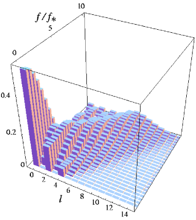
Figure 2: Angular power $\sigma_{\ell}(\hat{f})$ of the antenna pattern function for the toy model as a function of $\ell$ and $\hat{f}$.

V.2 Influence of transfer function

We now calculate the angular power of the antenna pattern fully taking into account the frequency and the angular dependences of the transfer function $\mathcal{T}$. The results are then compared with the toy model example. For this purpose, the spherical harmonic expansion of the antenna pattern function is numerically carried out using the SPHEREPACK 3.1 package (Adams and Swarztrauber, 2003).

Figure 3 shows the angular power of the antenna pattern function for the self-correlated Michelson signals $\mathcal{F}_{\scriptscriptstyle\rm M_{1}M_{1}}$(left) and the cross-correlated Michelson signals $\mathcal{F}_{\scriptscriptstyle\rm M_{1}M_{2}}$(right). Relaxation of the assumption $\mathcal{T}=\mbox{const.}$, i.e., low-frequency approximation, leads to the non-vanishing components for even modes with $\ell\geq 6$. However, the resultant higher multipole moments turn out to be highly suppressed. While the sensitivity to the higher multipole moments is slightly improved in the case of the cross-correlated Michelson signals, comparing it with Fig. 2 reveals that the frequency dependence of the transfer function $\mathcal{T}$ significantly reduces the angular power in both the lower and the higher multipole moments. The numerical evaluation of spherical harmonic expansion implies that the non-vanishing components of the angular power asymptotically decrease as $\sigma_{\ell}\propto\hat{f}^{-2}$ in the high frequency region, even faster than that of the toy model example.

The behaviors of the angular power are qualitatively similar to the case adopting the Sagnac variables that cancel the laser frequency noise (Fig.4). Apart from the low-frequency limit, where the antenna pattern function for Sagnac signals behaves as $\mathcal{F}_{\scriptscriptstyle{\rm S}_{i}{\rm S}_{j}}\sim\hat{f}^{2}$ [see Eqs. (46) and (48)], the angular power is highly suppressed at the frequency $\hat{f}\gtrsim 1$ even in the relatively lower multipole moments $\ell\lesssim 6$. Thus, the directional sensitivity of the space interferometer to a stochastic background of gravitational waves is severely limited by the frequency dependence of the transfer function. This fact is irrelevant to the choice of the interferometric variables.

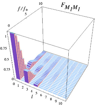
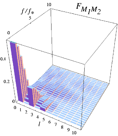
Figure 3: Angular power $\sigma_{\ell}(\hat{f})$ of the antenna pattern function for the self-correlated Michelson signals $\mathcal{F}_{\scriptscriptstyle\rm M_{1}M_{1}}$(left) and the cross-correlated Michelson signals, $\mathcal{F}_{\scriptscriptstyle\rm M_{1}M_{2}}$ (right).

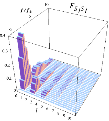
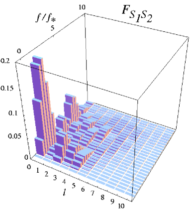
Figure 4: Angular power $\sigma_{\ell}(\hat{f})$ of the antenna pattern function for the self-correlated Sagnac signals $\mathcal{F}_{\scriptscriptstyle\rm S_{1}S_{1}}$ (left) and the cross-correlated Sagnac signals $\mathcal{F}_{\scriptscriptstyle\rm S_{1}S_{2}}$(right) .

V.3 Directional sensitivity for optimal combinations of TDI variables

To elucidate a more quantitative aspect of the directional sensitivity to the gravitational-wave background, it will need to take into account effects of detector noises. To investigate this, rather than using the Michelson and Sagnac signals, a set of optimal TDIs (A, E, T) free from the noise correlations should be applied to the correlation analysis of the gravitational-wave signals.

Figure 5 plots the quantity $\sigma_{\ell}$ for various combinations of the optimal TDIs. Note that the angular power of the antenna pattern function $\mathcal{F}_{\scriptscriptstyle\rm EE}$ ($\mathcal{F}_{\scriptscriptstyle\rm ET}$) coincides with that obtained from $\mathcal{F}_{\scriptscriptstyle\rm AA}$ ($\mathcal{F}_{\scriptscriptstyle\rm AT}$), although the sky patterns themselves differ from each other. For the self-correlated signals, the amplitude $\sigma_{\ell}$ of $\mathcal{F}_{\scriptscriptstyle\rm AA}$ is quite similar to that of the self-correlated Sagnac signals $\mathcal{F}_{\scriptscriptstyle\rm S_{1}S_{1}}$, while the low-frequency part of the angular power for $\mathcal{F}_{\scriptscriptstyle\rm TT}$ is highly suppressed, which can be deduced from the low-frequency approximation presented in Appendix A. As for the cross-correlation signals, the monopole and the dipole moments for the antenna pattern function $\mathcal{F}_{\scriptscriptstyle\rm AE}$ are exactly canceled and the monopole moment for $\mathcal{F}_{\scriptscriptstyle\rm AT}$ further vanishes (Table 1 and Appendix C). Apart from these facts, the magnitude $\sigma_{\ell}$ at frequency $\hat{f}\gtrsim 1$ shows a rich structure with many peaks, indicating that the directional sensitivity could be improved at $\hat{f}\gtrsim 1$. As shown in Fig. 5, the angular power of the cross-correlated signals is one order of magnitude smaller than that of the self-correlated signals, however, this does not directly imply that the self-correlated signals are more sensitive to an anisotropy of a gravitational-wave background.

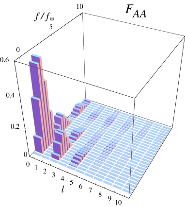
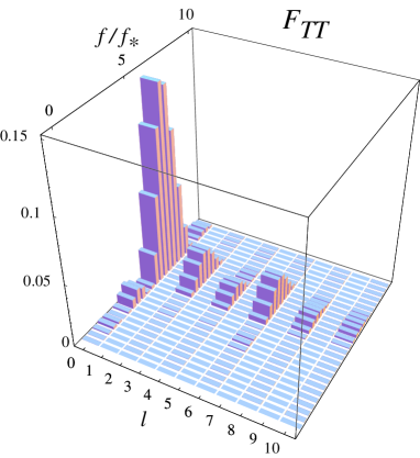
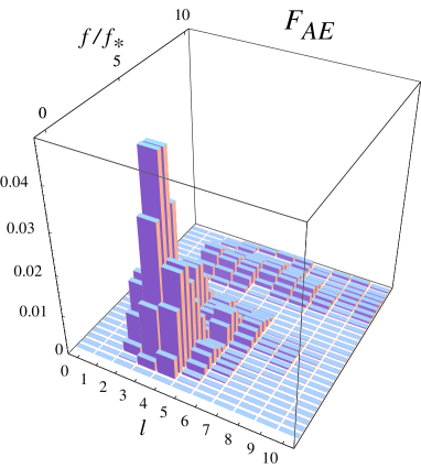
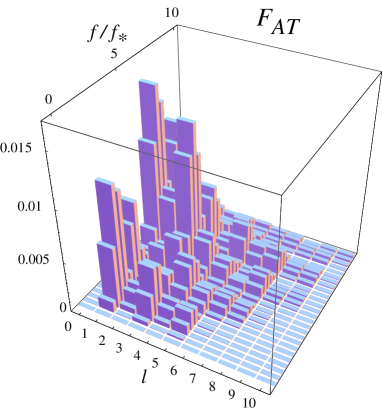
Figure 5: Angular power $\sigma_{\ell}(\hat{f})$ of the antenna pattern functions for the optimal TDI variables. The top panels show the magnitude $\sigma_{\ell}$ in the self-correlated cases $\mathcal{F}_{\scriptscriptstyle\rm AA}$(left) and $\mathcal{F}_{\scriptscriptstyle\rm TT}$(right), while the bottom panels represent the results obtained from the cross-correlated signals $\mathcal{F}_{\scriptscriptstyle\rm AE}$(left) and $\mathcal{F}_{\scriptscriptstyle\rm AT}$(right). Note that the angular powers of antenna pattern $\mathcal{F}_{\scriptscriptstyle\rm EE}$ and $\mathcal{F}_{\scriptscriptstyle\rm ET}$ coincide with those of $\mathcal{F}_{\scriptscriptstyle\rm AA}$ and $\mathcal{F}_{\scriptscriptstyle\rm AT}$.

Based on these results, let us now quantify the directional sensitivity of the antenna pattern function. Assuming that the laser frequency noise can be either canceled or sufficiently reduced by the TDI technique with the use of the recently proposed laser self-locking scheme Sheard et al. (2003); Sylvestre (2004), the dominant noise contributions to detector’s output would be the acceleration noise and the shot noise. According to Ref. Cornish (2002b), the noise spectral densities for optimal TDIs are calculated as (see also Prince et al. (2002)):

$$S_{n}^{\scriptscriptstyle\rm AA}(f) = S_{n}^{\scriptscriptstyle\rm EE}(f)=\sin^{2}(\hat{f}/2)\,\,\left\{8\,\left(2+\cos\hat{f}\right)\,\,S_{\rm shot}(f)+16\,\left(3+2\cos\hat{f}+\cos 2\hat{f}\right)\,\,S_{\rm accel}(f)\right\},$$ (82)

$$S_{n}^{\scriptscriptstyle\rm TT}(f) = 2\,\,\left(1+2\cos\hat{f}\right)^{2}\left\{S_{\rm shot}(f)+4\sin^{2}(\hat{f}/2)\,\,S_{\rm accel}(f)\right\}.$$ (83)

Note that the cross-correlated noise spectra are exactly canceled. Here we specifically adopt the noise functions for the LISA detector: $S_{\rm shot}(f)=4.84^{-42}$Hz^-1 and $S_{\rm accel}(f)=2.31^{-40}(\mbox{mHz}/f)^{4}$Hz^-1Cornish (2002b). We then define the effective sensitivity for the multipole moment $\ell$, $h_{\rm eff}^{(\ell)}(f)$, which characterizes the rms amplitude of the noise-to-angular power ratio:

$$h^{(\ell)}_{\rm eff}(f)=(4\pi)^{1/4}\,\,\sqrt{\frac{S_{\rm n}(f)}{\sigma_{\ell}(f)}}$$ (84)

for self-correlation signals. Setting $\ell=0$, the above definition recovers the usual meaning of sensitivity curve. Thus, the quantity $h_{\rm eff}^{(\ell)}(f)$ may be regarded as the effective power of $\ell$-th moment relative to the monopole moment as a reference sensitivity. For the cross-correlated signals, on the other hand, the absence of noise correlation implies that the signal-to-noise ratio can be improved by optimally filtering the cross-correlated signals. The resultant form of the signal-to-noise ratio shows the explicit dependence on the observation time $T$ Allen and Romano (1999). According to Ref. Cornish (2002b), the effective sensitivity for cross-correlated signals may be written as:

$$h_{\rm eff}^{(\ell)}(f)=\left(\frac{4\pi}{T\Delta f}\right)^{1/4}\,\left[\frac{S_{n,1}(f)\,\,S_{n,2}(f)}{\sigma^{2}_{\ell}(\hat{f})}\right]^{1/4},$$ (85)

where $\Delta f$ denotes the frequency resolution for actual output data.

Figure 6 shows the effective sensitivity curves for the self-correlated and cross-correlated optimal TDIs as functions of $\hat{f}=f/f_{*}$. In plotting these curves, we used the characteristic frequency $f_{*}\simeq 10$mHz for the LISA detector. The different lines in each panel indicate the effective strain sensitivity for each multipole moment. Clearly, the directional sensitivity to a gravitational-wave background is not so good in the case of the self-correlated signals. As anticipated from Figure 5 and the noise spectra (83), the effective sensitivity in the low-frequency limit scales as $h_{\rm eff}^{(\ell)}\propto f^{-2}$ for $\ell=0,\,2$ and $4$ of AA-correlation and $h_{\rm eff}^{(\ell)}\propto f^{-3}$ for $\ell=0,\,4$ and $6$ of TT-correlation. At the frequency around the characteristic frequency $f_{*}$, the directional sensitivities may reach at a maximal level and the higher multipole moment can be observed in both AA- and TT-correlations, however, the detectable multipole moments are still limited to $\ell=$even mode with $\ell\lesssim 6$ for the sensitivity $h_{\rm eff}^{(\ell)}\sim 10^{-18}$ Hz^-1/2.

The situation might be improved if we consider the cross-correlation signals. In bottom panels of Figure 6, the observation time of $T=1$ year and the frequency resolution with interval $\Delta f=f/10$ are assumed. In this case, the sensitivity reaches $h_{\rm eff}^{(\ell)}\sim 5\times 10^{-21}$Hz^-1/2 in both AE- and AT-correlations (and also the ET-correlation), and the detectable multipole moments become, say, $\ell\lesssim 10$ or even higher multipole moments in both $\ell=$odd and even modes. At the frequency $f/f_{*}\sim 3$, the effective sensitivity for the higher multipole moments becomes comparable to that for the lower multipole and shows a complicated oscillatory behavior. Although the antenna pattern for cross-correlation signals is completely insensitive to the $\ell=0$ mode, improvement of the sensitivity is noticeable, which might be useful to distinguish between the gravitational-wave backgrounds from Galactic origin and those from extragalactic origin.

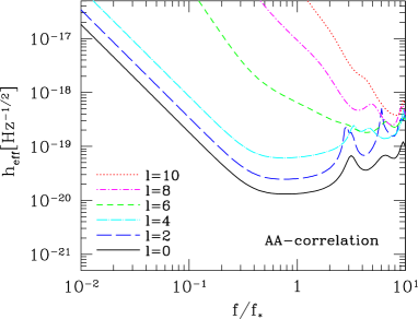
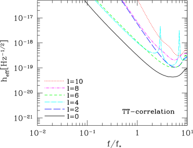
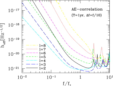
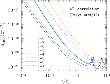
Figure 6: Effective sensitivity curves defined in (84) and (85) for the self-correlated and cross-correlated optimal TDI variables: AA-correlation(top-left); TT-correlation(top-right); AE-correlation(bottom-left); AT-correlation(bottom-right). In cases of the cross-correlation signals depicted in bottom panels, the observation time of $T=1$ year and the frequency resolution $\Delta f=f/10$ are assumed. The characteristic frequency is $f_{*}\simeq 10$mHz.

VI Conclusion & Discussions

In this paper, we discussed the directional sensitivity to the anisotropy of gravitational-wave background observed via space-based gravitational-wave detector. While the detection of anisotropic gravitational-wave background could be achieved utilizing the modulated signals of cross-correlated data induced by the detector motion, the directional sensitivity and the angular resolution crucially depend on the antenna pattern function and/or the detector response in detector’s rest frame. In contrast to the groundbased detector, the space interferometer with long baselines gives a rather complicated response to the gravitational-wave signals.

We have performed the spherical harmonic analysis of antenna pattern function for space interferometer and studied the general features of antenna pattern sensitivity beyond the low-frequency approximation. We have shown that the sensitivity to the multipole moments of an anisotropic gravitational-wave background is generally restricted by the geometry of the detector configuration and symmetries of the data combinations (see Table 1, Sec. IV.3 and Sec. IV.4). The numerical analysis of the antenna pattern functions reveals that the angular power of the detector response increases with frequency and shows the complicated structures. To characterize the directional sensitivity, we introduced the effective sensitivity $h_{\rm eff}^{(\ell)}(f)$ for each multipole moment and evaluated it in the case of the LISA detector specifically. Using the cross-correlated data of optimal TDIs, i.e., AE-, AT- and ET-correlations, we found that the detectable multipole moments with effective sensitivity $h_{\rm eff}^{(\ell)}\sim 10^{-20}$Hz^-1/2 may reach $\ell=8\sim 10$ or even higher multipoles at $f\sim f_{*}=10$ mHz, which would be useful to discriminate between the gravitational-wave backgrounds of Galactic origin and those of the extragalactic and/or the cosmological origins, recently discussed by several authors (e.g., Kosenko and Postnov (1998); Schneider et al. (2001); Farmer and Phinney (2003)).

Although the improvement of the directional sensitivity beyond the low-frequency approximation is remarkable, the sensitivity of the space interferometer is still worse than the one achieved by the cosmic microwave background experiments, like the COBE (cosmic background explorer) and WMAP (Wilkinson microwave anisotropy probe). The one main reason is that the wavelength of the gravitational waves to which the space interferometer is sensitive is comparable to or longer than the arm length of the detector. Because of this, the response to the gravitational-wave background becomes simpler and most of the directional information is lost, as seen in Sec.IV.2. The directional sensitivity can be improved as increasing the frequency, however, the sensitivity beyond the characteristic frequency $f_{*}$ is limited by the instrumental noises. Another important aspect is that the phases of the gravitational-wave backgrounds are, in nature, random. Thus, the information of phase modulation induced by the detector motion cannot be used. This is marked contrast to the signals emitted from the point source, in which the angular resolution can reach at a level of a square degree or even better than that  Cutler (1998); Moore and Hellings (2002); Peterseim et al. (1997); Takahashi and Nakamura (2003); Seto (2002).

Further notice the important issues concerning the map-making capability of the gravitational-wave backgrounds. As discussed in Sec.II, provided the time series data, the task is to solve the linear system (16) under a prior knowledge of the antenna pattern functions for the space interferometer. The crucial remark is that the antenna pattern functions for the cross-correlation signals taken from the optimal TDIs (A, E, T) are not independent (see Sec.IV.4). This fact implies that Eq. (16) constructed from the three cross-correlation data (AE, AT, ET) is generally degenerate. Thus, the deconvolution problem given in (16) would not be solved rigorously. Rather, one must seek a best-fit solution of $p_{\ell m}^{E}(f)$ from (16) under assuming a specific functional form of the luminosity distribution $p_{\ell m}^{E}(f)$. The analysis concerning this issue is now in progress and will be presented elsewhere.

Appendix A Spherical harmonic expansion in the low-frequency approximation

In this appendix, employing the perturbative approach based on the low-frequency approximation $\hat{f}=f/f_{*}\ll 1$, the spherical harmonic expansions for several antenna patterns are presented, which partially verify the properties summarized in Table 1 and Eq. (51).

A.1 Sagnac interferometers

The angular powers $\sigma_{\ell}$ of the self-correlated Sagnac signal $\mathcal{F}_{\scriptscriptstyle{\rm S}_{i}{\rm S}_{i}}$ and the cross-correlated Sagnac signal $\mathcal{F}_{\scriptscriptstyle{\rm S}_{i}{\rm S}_{j}}$ in the low-frequency approximation are summarized as follows:

$$\mathcal{F}_{\scriptscriptstyle{\rm S}_{i}{\rm S}_{i}}: \sigma_{0}=\frac{4\sqrt{\pi}\,{\hat{f}}^{2}}{15}-\frac{839\sqrt{\pi}\,{\hat{f}}^{4}}{7560},\quad\sigma_{2}=\frac{8\sqrt{\pi}\,{\hat{f}}^{2}}{105}-\frac{32\sqrt{\pi}\,{\hat{f}}^{4}}{945},\quad\sigma_{4}=\frac{4\sqrt{\pi}\,{\hat{f}}^{2}}{315}-\frac{5233\sqrt{\pi}\,{\hat{f}}^{4}}{997920},$$

$$\sigma_{6}=\frac{\sqrt{\pi}\,}{432432}\sqrt{\frac{51641}{15}}{\hat{f}}^{4},$$

$$\mathcal{F}_{\scriptscriptstyle{\rm S}_{i}{\rm S}_{j}}: \sigma_{0}=\frac{2\sqrt{\pi}\,{\hat{f}}^{2}}{15}-\frac{61\sqrt{\pi}\,{\hat{f}}^{4}}{1080},\quad\sigma_{1}=\frac{\sqrt{\pi}\,{\hat{f}}^{3}}{126},\quad\sigma_{2}=\frac{4\sqrt{\pi}\,{\hat{f}}^{2}}{105}-\frac{16\sqrt{\pi}\,{\hat{f}}^{4}}{945},\quad\sigma_{3}=\frac{\sqrt{\pi}\,}{378}\sqrt{\frac{211}{10}}{\hat{f}}^{3},$$ (86)

$$\sigma_{4}=\frac{\sqrt{\pi}}{315}\sqrt{\frac{47}{3}}{\hat{f}}^{2}-\frac{12889\sqrt{\pi}}{166320\sqrt{141}}{\hat{f}}^{4},\quad\sigma_{5}=\frac{\sqrt{\pi}\,}{8316}\sqrt{\frac{689}{5}}{\hat{f}}^{3},\quad\sigma_{6}=\frac{\sqrt{\pi}\,}{4752}\sqrt{\frac{311}{1365}}{\hat{f}}^{4}.$$ (87)

A.2 Optimal combinations of time-delay interferometry

From Eq. (35) the antenna pattern functions of the self-correlated optimal TDIs can be written down in terms of the antenna pattern for the Sagnac signals:

$$\mathcal{F}_{\scriptscriptstyle\rm AA}=\frac{1}{2}\left\{\mathcal{F}_{\scriptscriptstyle 33}+\mathcal{F}_{\scriptscriptstyle 11}-\mathcal{F}_{\scriptscriptstyle{(1,3)}}\right\},$$ (88)

$$\mathcal{F}_{\scriptscriptstyle\rm EE}=\frac{1}{{6}}\left\{\mathcal{F}_{\scriptscriptstyle 11}+4\mathcal{F}_{\scriptscriptstyle 22}+\mathcal{F}_{\scriptscriptstyle 33}+\mathcal{F}_{\scriptscriptstyle{(1,3)}}-2\mathcal{F}_{\scriptscriptstyle{(1,2)}}-2\mathcal{F}_{\scriptscriptstyle{(2,3)}}\right\},$$ (89)

$$\mathcal{F}_{\scriptscriptstyle\rm TT}=\frac{1}{3}\left\{\mathcal{F}_{\scriptscriptstyle 11}+\mathcal{F}_{\scriptscriptstyle 22}+\mathcal{F}_{\scriptscriptstyle 33}+\mathcal{F}_{\scriptscriptstyle{(1,3)}}+\mathcal{F}_{\scriptscriptstyle{(1,2)}}+\mathcal{F}_{\scriptscriptstyle{(2,3)}}\right\}.$$ (90)

where the round brackets are an abbreviation for the symmetrization, $\mathcal{F}_{\scriptscriptstyle{(1,3)}}=\mathcal{F}_{\scriptscriptstyle{1}{3}}+\mathcal{F}_{\scriptscriptstyle{3}{1}}$ for instance, and $\mathcal{F}_{\scriptscriptstyle ij}$ stands for $\mathcal{F}_{\scriptscriptstyle{\rm S}_{i}{\rm S}_{j}}$. The antenna pattern functions of the cross-correlated signals, $\mathcal{F}_{\scriptscriptstyle\rm AE}$, $\mathcal{F}_{\scriptscriptstyle\rm AT}$ and $\mathcal{F}_{\scriptscriptstyle\rm ET}$, are

$$\mathcal{F}_{\scriptscriptstyle\rm AE}=\frac{1}{2\sqrt{3}}\left\{\mathcal{F}_{\scriptscriptstyle 33}-\mathcal{F}_{\scriptscriptstyle 11}+\mathcal{F}_{\scriptscriptstyle 31}-\mathcal{F}_{\scriptscriptstyle 13}+2\mathcal{F}_{\scriptscriptstyle 12}-2\mathcal{F}_{\scriptscriptstyle 32}\right\},$$ (91)

$$\mathcal{F}_{\scriptscriptstyle\rm AT}=\frac{1}{\sqrt{6}}\left\{\mathcal{F}_{\scriptscriptstyle 33}-\mathcal{F}_{\scriptscriptstyle 11}+\mathcal{F}_{\scriptscriptstyle 31}-\mathcal{F}_{\scriptscriptstyle 13}+\mathcal{F}_{\scriptscriptstyle 32}-\mathcal{F}_{\scriptscriptstyle 12}\right\},$$ (92)

$$\mathcal{F}_{\scriptscriptstyle\rm ET}=\frac{1}{3\sqrt{2}}\left\{\mathcal{F}_{\scriptscriptstyle 11}-2\mathcal{F}_{\scriptscriptstyle 22}+\mathcal{F}_{\scriptscriptstyle 33}+\mathcal{F}_{\scriptscriptstyle 12}-2\mathcal{F}_{\scriptscriptstyle 21}+\mathcal{F}_{\scriptscriptstyle 32}-2\mathcal{F}_{\scriptscriptstyle 23}+\mathcal{F}_{\scriptscriptstyle{(1,3)}}\right\}.$$ (93)

Under the configuration in a specific coordinate (42), the low-frequency approximation of the multipole coefficients of the self-correlated optimal variables are given as follows:

$$\mathcal{F}_{\scriptscriptstyle\rm AA}:\quad a_{{00}}=\frac{2\sqrt{\pi}}{5}{\hat{f}}^{2},\quad a_{{20}}=\frac{4}{7}\sqrt{\frac{\pi}{5}}{\hat{f}}^{2},\quad a_{{40}}=\frac{\sqrt{\pi}}{105}{\hat{f}}^{2},\quad a_{{44}}=-\left(\frac{1}{6}\sqrt{\frac{\pi}{70}}+\frac{i}{2}\sqrt{\frac{\pi}{210}}\right){\hat{f}}^{2},$$

$$\mathcal{F}_{\scriptscriptstyle\rm EE}:\quad a_{{00}}=\frac{2\sqrt{\pi}}{5}{\hat{f}}^{2},\quad a_{{20}}=\frac{4}{7}\sqrt{\frac{\pi}{5}}{\hat{f}}^{2},\quad a_{{40}}=\frac{\sqrt{\pi}}{105}{\hat{f}}^{2},\quad a_{{44}}=\left(\frac{1}{6}\sqrt{\frac{\pi}{70}}+\frac{i}{2}\sqrt{\frac{\pi}{210}}\right){\hat{f}}^{2},$$

$$\mathcal{F}_{\scriptscriptstyle\rm TT}:\quad a_{{00}}=\frac{\sqrt{\pi}}{504}{\hat{f}}^{4},\quad a_{{40}}=-\frac{\sqrt{\pi}}{1584}{\hat{f}}^{4},\quad a_{{60}}=-\frac{\sqrt{\pi}}{11088\sqrt{13}}{\hat{f}}^{4},\quad a_{{66}}=-\frac{\sqrt{\pi}}{48\sqrt{3003}}{\hat{f}}^{4}.$$ (94)

$m<0$ modes are given by the relation (41). The rule (51) strictly restricts the appearance of multipole moments, and of course the above multipole moments follow the rule (51). For the cross-correlation of two data streams, one would expect that $\ell=$ odd modes appear even in the low-frequency limit. However it is not the case. A non-vanishing multipole moment is given to order $\mathcal{O}({\hat{f}}^{2})$ by

$$\mathcal{F}_{\scriptscriptstyle\rm AE}:\quad \quad a_{{44}}=\left(\frac{1}{2\sqrt{210}}-\frac{i}{6\sqrt{70}}\right)\sqrt{\pi}{\hat{f}}^{2}.$$ (95)

The $\ell=$ odd modes appear in the next order $\mathcal{O}(\hat{f}^{3})$ in some multipole moments that satisfy $\ell+m=\mathrm{even}$:

$$\mathcal{F}_{\scriptscriptstyle\rm AE}:\quad a_{{33}}=\frac{1}{18}\sqrt{\frac{7\pi}{15}}{\hat{f}}^{3},\quad a_{{53}}=\frac{1}{18}\sqrt{\frac{\pi}{1155}}{\hat{f}}^{3},$$ (96)

The angular powers up to $\mathcal{O}(\hat{f}^{4})$ are summarized as

$$\mathcal{F}_{\scriptscriptstyle\rm AA},\mathcal{F}_{\scriptscriptstyle\rm EE} : \sigma_{0}=\frac{2\sqrt{\pi}}{5}{\hat{f}}^{2}-\frac{211\sqrt{\pi}}{1260}{\hat{f}}^{4}, \sigma_{2}=\frac{4\sqrt{\pi}}{35}{\hat{f}}^{2}-\frac{16\sqrt{\pi}}{315}{\hat{f}}^{4}, \sigma_{4}=\frac{2\sqrt{\pi}}{105}{\hat{f}}^{2}-\frac{4511\sqrt{\pi}}{498960}{\hat{f}}^{4}, \sigma_{6}=\frac{\sqrt{\pi}}{72072}\sqrt{\frac{1829}{15}}{\hat{f}}^{4},$$

$$\mathcal{F}_{\scriptscriptstyle\rm TT} : \sigma_{0}=\frac{\sqrt{\pi}}{504}{\hat{f}}^{4}, \sigma_{4}=\frac{\sqrt{\pi}}{4752}{\hat{f}}^{4}, \sigma_{6}=\frac{\sqrt{\pi}\,\sqrt{463}}{144144}{\hat{f}}^{4}$$ (97)

and

$$\mathcal{F}_{\scriptscriptstyle\rm AE}:\quad \sigma_{0}=0,\quad\sigma_{1}=0,\quad\sigma_{2}=\frac{{\sqrt{\pi}\hat{f}^{4}}}{126\sqrt{3}},\quad\sigma_{3}=\frac{{\sqrt{\pi}\hat{f}^{3}}}{9\sqrt{30}},$$ (98)

$$\sigma_{4}=\frac{\sqrt{\pi}}{9\sqrt{35}}{\hat{f}^{2}}-\frac{13\sqrt{\pi}}{1188}\sqrt{\frac{5}{7}}{\hat{f}^{4}},\quad\sigma_{5}=\frac{{\hat{f}}^{3}}{99\sqrt{210}},\quad\sigma_{6}=\frac{{\sqrt{\pi}\hat{f}^{4}}}{468\sqrt{210}}.$$

Appendix B Parity transformation

Here, we summarize some formulae related to the parity transformation, which are used in Sec.IV.3. In general, parity of the polarization tensor $\mathbf{e}^{+,\times}$ depends on the choice of the coordinate basis. Our choice of the basis vectors are those defined in (4) and (7) just simply replacing the variables $\theta_{E},\phi_{E}$ with $\theta,\phi$ in detector’s rest frame. In the following, the vector ${\bf d}$ stands for the unit vectors ${\bf a},{\bf b},{\bf c}$. We then obtain

$${\mathbb{P}}\,({\bf d}\cdot{\bf\Omega}) = -1~{}({\bf d}\cdot{\bf\Omega}),$$

$${\mathbb{P}}\,({\bf d}\otimes{\bf d}):\mathbf{e}^{A} = +1~{}({\bf d}\otimes{\bf d}):\mathbf{e}^{A}\quad(A=+,\times)$$ (99)

for the operator $\mathbb{P}$ and

$${\mathbb{Q}}\,({\bf d}\cdot{\bf\Omega}) = +1~{}({\bf d}\cdot{\bf\Omega}),$$

$${\mathbb{Q}}\,({\bf d}\otimes{\bf d}):\mathbf{e}^{+} = +1~{}({\bf d}\otimes{\bf d}):\mathbf{e}^{+},$$

$${\mathbb{Q}}\,({\bf d}\otimes{\bf d}):\mathbf{e}^{\times} = -1~{}({\bf d}\otimes{\bf d}):\mathbf{e}^{\times}$$ (100)

for the operator $\mathbb{Q}$. As for the composite operation $\mathbb{QP}$, which is identical to the parity transformation, one has

$${\mathbb{Q\,P}}\,({\bf d}\cdot{\bf\Omega}) = -1~{}({\bf d}\cdot{\bf\Omega}),$$

$${\mathbb{Q\,P}}\,({\bf d}\otimes{\bf d}):\mathbf{e}^{+} = +1~{}({\bf d}\otimes{\bf d}):\mathbf{e}^{+},$$

$${\mathbb{Q\,P}}\,({\bf d}\otimes{\bf d}):\mathbf{e}^{\times} = -1~{}({\bf d}\otimes{\bf d}):\mathbf{e}^{\times}.$$ (101)

Appendix C On cancellation of monopole and dipole moments in antenna pattern function for cross-correlated optimal TDIs

In this appendix, we will prove that the antenna pattern function for the cross-correlated optimal TDIs has the following symmetric properties:

$$\sigma_{0}(f)=0,\quad\sigma_{1}(f)=0~{}~{}~{}\mbox{for AE-correlation},$$ (102)

$$\sigma_{0}(f)=0\quad\quad\quad\quad~{}~{}~{}~{}~{}~{}~{}~{}\mbox{for AT-,ET-correlation},$$ (103)

which are intimately related to the geometric properties of both the detector configuration and the response function. As we have explained, the antenna pattern functions $\mathcal{F}_{\scriptscriptstyle\rm AE}$, $\mathcal{F}_{\scriptscriptstyle\rm AT}$ and $\mathcal{F}_{\scriptscriptstyle\rm ET}$ are written in terms of the antenna pattern functions for the Sagnac signals [see Eq. (93)]. The expressions readily imply that the multipole moments for the antenna pattern functions, $a_{\ell m}^{\scriptscriptstyle\rm AE}$, $a_{\ell m}^{\scriptscriptstyle\rm AT}$ and $a_{\ell m}^{\scriptscriptstyle\rm ET}$, are also obtained from the sum of the cross-correlated Sagnac signals, $a_{\ell m}^{\scriptscriptstyle{\rm S}_{i}{\rm S}_{j}}$ [see (64), for example].

Let us first consider the monopole moment $a_{00}$. Since the monopole moment is obtained through the all-sky average of the antenna pattern function, it is, by construction, invariant under both the Euler rotation and the parity transformation of the coordinate system. This indicates that the monopole moments for various combinations of the Sagnac signals $a_{\ell m}^{\scriptscriptstyle{\rm S}_{i}{\rm S}_{j}}$ are degenerate and there are only two independent variables, that is,

$$a_{00}^{\scriptscriptstyle\rm S_{1}S_{1}}=a_{00}^{\scriptscriptstyle\rm S_{2}S_{2}}=a_{00}^{\scriptscriptstyle\rm S_{3}S_{3}},\quad\quad a_{00}^{\scriptscriptstyle{\rm S}_{i}{\rm S}_{j}}=a_{00}^{\scriptscriptstyle{\rm S}_{k}{\rm S}_{l}}~{}~{}(i\neq j,~{}k\neq l).$$ (104)

Substituting this into the spherical harmonic expansion of the antenna pattern functions (93), we immediately see that the monopole component of cross-correlated optimal signals exactly vanishes, i.e., $a_{00}^{\scriptscriptstyle\rm AE}=a_{00}^{\scriptscriptstyle\rm AT}=a_{00}^{\scriptscriptstyle\rm ET}=0$. Accordingly, the monopole moments of angular power, $\sigma_{0}^{\scriptscriptstyle\rm AE}$, $\sigma_{0}^{\scriptscriptstyle\rm AT}$ and $\sigma_{0}^{\scriptscriptstyle\rm ET}$, become vanishing.

Next focus on the dipole moment of AE correlation. In a specific choice of the coordinate system (42), all the components in the dipole moment vanish due to Eq. (51) for the self-correlated Sagnac signals, i.e., $a_{1,m}^{\scriptscriptstyle{\rm S}_{i}{\rm S}_{i}}=0$. Also, the dipole moment with $m=0$ becomes zero for the cross-correlated signals, i.e., $a_{10}^{\scriptscriptstyle{\rm S}_{i}{\rm S}_{j}}=0$. Further, the relation (41) implies $a_{1,-1}^{\scriptscriptstyle\rm AE}=[a_{11}^{\scriptscriptstyle\rm AE}]^{*}$. Collecting these facts, the dipole moment of angular power $\sigma_{1}^{\scriptscriptstyle\rm AE}$ can be written as

$$\sigma^{\scriptscriptstyle\rm AE}_{1}=\sqrt{\frac{2}{3}}\,\,|a^{\scriptscriptstyle\rm AE}_{11}|=\frac{1}{3\sqrt{2}}\left|a_{11}^{\scriptscriptstyle\rm S_{3}S_{1}}-a_{11}^{\scriptscriptstyle\rm S_{1}S_{3}}+2a_{11}^{\scriptscriptstyle\rm S_{1}S_{2}}-2a_{11}^{\scriptscriptstyle\rm S_{3}S_{2}}\right|.$$ (105)

It is thus sufficient to consider the dipole moment with $m=+1$ for the cross-correlated Sagnac signals.

From Eq. (61), the angular power $\sigma_{1}^{\scriptscriptstyle\rm AE}$ can be solely determined by the quantity $a_{11}^{S_{1}S_{2}}$. If we write $a_{11}^{\scriptscriptstyle\rm S_{1}S_{2}}=r(\hat{f})\,e^{i\theta(\hat{f})}$, Eq. (105) becomes

$$\sigma_{1}^{\scriptscriptstyle\rm AE}(\hat{f})=\frac{r}{3\sqrt{2}}\,\,\left|2+e^{-i\,2\delta}+\left(1+2\,e^{-i\,2\delta}\right)\,e^{-i\,2\theta}\right|_{\delta=2\pi/3}.$$ (106)

To determine the phase factor $\theta(\hat{f})$ or amplitude $r(\hat{f})$, we recall the fact that the dipole moment of antenna pattern function $\mathcal{F}_{\scriptscriptstyle\rm AA}$ vanishes:

$$a_{11}^{\scriptscriptstyle\rm AA} = \frac{1}{2}\left(a_{11}^{\scriptscriptstyle\rm S_{1}S_{1}}+a_{11}^{\scriptscriptstyle\rm S_{3}S_{3}}-a_{11}^{\scriptscriptstyle\rm S_{1}S_{3}}-a_{11}^{\scriptscriptstyle\rm S_{3}S_{1}}\right)=-\frac{1}{2}\left(a_{11}^{\scriptscriptstyle\rm S_{1}S_{3}}+a_{11}^{\scriptscriptstyle\rm S_{3}S_{1}}\right)$$

$$= 0.$$

from (35). Using the relations (61), the above equation becomes

$$a_{11}^{\scriptscriptstyle\rm AA}=\frac{r\,e^{i\,\theta}}{2}\left(e^{-i\,2\theta}-e^{-i\,2\delta}\right)_{\delta=2\pi/3}=0,$$

which finally yields $r(\hat{f})=0$ or $\theta(\hat{f})=\delta+n\pi$. Thus, substituting this value into the right-hand-side of equation (106) immediately leads to the conclusion that the dipole moment of angular power $\sigma_{1}^{\scriptscriptstyle\rm AE}$ is exactly canceled. This means that all the dipole components for $a_{\ell m}^{\scriptscriptstyle\rm AE}$ become zero over the whole frequency range.

Appendix D Coefficients in antenna pattern for toy model

In this appendix, we summarize the coefficients $c^{(m,N)}$ and the functions $g_{s}^{(m,N)}(\hat{f})$ defined in (76) and (78).

For the coefficients $c^{(m,N)}$, the non-vanishing components are

$$c^{(0,0)}=-\frac{123\pi}{256},~{}~{}c^{(0,1)}=\frac{135\pi}{128},~{}~{}c^{(0,2)}=-\frac{219\pi}{256},$$

$$c^{(2,0)}=-\frac{15\pi}{128},~{}~{}c^{(2,1)}=-\frac{39\pi}{128},$$

$$c^{(4,0)}=-\frac{9\pi}{512}.$$ (107)

As for the functions $g_{s}^{(m,N)}(\hat{f})$, the non-vanishing components for $0\leq m\leq 4$ and $0\leq N\leq 2$ become

$$\begin{array}[]{llll}g_{0}^{(0,0)}=1,&g_{0}^{(2,0)}=-4-\hat{f}^{2},&g_{0}^{(2,1)}=2,&g_{0}^{(4,0)}=144+48\hat{f}^{2}+\hat{f}^{4},\\ \\ g_{1}^{(2,0)}=8i\,\hat{f},&g_{1}^{(2,1)}=-4i\,\hat{f},&g_{1}^{(4,0)}=-576i\,\hat{f}-32i\,\hat{f}^{3},&\\ \\ g_{2}^{(0,1)}=1,&g_{2}^{(2,0)}=12+2\hat{f}^{2},&g_{2}^{(2,1)}=-24-\hat{f}^{2},&g_{2}^{(4,0)}=-1440-432\hat{f}^{2}-4\hat{f}^{4},\\ \\ g_{3}^{(2,0)}=-8i\,\hat{f},&g_{3}^{(2,1)}=16i\,\hat{f},&g_{3}^{(4,0)}=1920i\,\hat{f}+96i\,\hat{f}^{3},&\\ \\ g_{4}^{(0,2)}=1,&g_{4}^{(2,0)}=-\hat{f}^{2},&g_{4}^{(2,1)}=30+2\hat{f}^{2},&g_{4}^{(4,0)}=1680+720\hat{f}^{2}+6\hat{f}^{4},\\ \\ g_{5}^{(2,1)}=-12i\,\hat{f},&g_{5}^{(4,0)}=-1344i\,\hat{f}-96i\hat{f}^{3},&&\\ \\ g_{6}^{(2,1)}=-\hat{f}^{2},&g_{6}^{(4,0)}=-336\hat{f}^{2}-4\hat{f}^{4},&&\\ \\ g_{7}^{(4,0)}=32i\,\hat{f}^{3},&&&\\ \\ g_{8}^{(4,0)}=\hat{f}^{4}.&&&\end{array}$$ (125)

Note that the other components with $m\geq 0$ do not contribute to the calculation of the multipole coefficient $a_{\ell m}$ due to the coefficients $c^{(m,N)}$ (Eq. (107)).

References

• Seto et al. (2001) N. Seto, S. Kawamura, and T. Nakamura, Phys. Rev. Lett. 87, 221103 (2001), eprint astro-ph/0108011.
• Takahashi and Nakamura (2003) R. Takahashi and T. Nakamura, Astrophys. J. 596, L231 (2003), eprint astro-ph/0307390.
• BBO (2003) See http://universe.gsfc.nasa.gov/be/roadmap.html (2003).
• Vallisneri (2004) M. Vallisneri (2004), eprint gr-qc/0407102.
• Cor (2003) see also LISA Simulator v. 2.0, http://www.physics.montana.edu/lisa/ (2003).
• Cornish and Rubbo (2003) N. J. Cornish and L. J. Rubbo, Phys. Rev. D67, 022001 (2003), eprint gr-qc/0209011.
• Merkowitz (2003) S. M. Merkowitz, Class. Quant. Grav. 20, S255 (2003).
• Merkowitz et al. (2004) S. M. Merkowitz et al., Class. Quant. Grav. 21, S603 (2004).
• Cutler (1998) C. Cutler, Phys. Rev. D57, 7089 (1998), eprint gr-qc/9703068.
• Tinto and Armstrong (1999) M. Tinto and J. W. Armstrong, Phys. Rev. D59, 102003 (1999).
• Armstrong et al. (1999) J. W. Armstrong, F. B. Estabrook, and M. Tinto, Astrophys. J. 527, 814 (1999).
• Dhurandhar et al. (2002) S. V. Dhurandhar, K. Rajesh Nayak, and J.-Y. Vinet, Phys. Rev. D65, 102002 (2002), eprint gr-qc/0112059.
• Prince et al. (2002) T. A. Prince, M. Tinto, S. L. Larson, and J. W. Armstrong, Phys. Rev. D66, 122002 (2002), eprint gr-qc/0209039.
• Krolak et al. (2004) A. Krolak, M. Tinto, and M. Vallisneri (2004), eprint gr-qc/0401108.
• Hils et al. (1990) D. Hils, P. L. Bender, and R. F. Webbink, Astrophys. J. 360, 75 (1990).
• Bender and Hils (1997) P. L. Bender and D. Hils, Class. Quant. Grav. 14, 1439 (1997).
• Nelemans et al. (2001) G. Nelemans, L. R. Yungelson, and S. F. Portegies Zwart, Astron. Astrophys. 375, 890 (2001), eprint astro-ph/0105221.
• Kosenko and Postnov (1998) D. I. Kosenko and K. A. Postnov, Astron. Astrophys. 336, 786 (1998).
• Schneider et al. (2001) R. Schneider, V. Ferrari, S. Matarrese, and S. F. Portegies Zwart, Mon. Not. Roy. Astron. Soc. 324, 797 (2001), eprint astro-ph/0002055.
• Farmer and Phinney (2003) A. J. Farmer and E. S. Phinney, Mon. Not. Roy. Astron. Soc. 346, 1197 (2003), eprint astro-ph/0304393.
• Maggiore (2000) M. Maggiore, Phys. Rept. 331, 283 (2000), eprint gr-qc/9909001.
• Giampieri and Polnarev (1997a) G. Giampieri and A. G. Polnarev, Mon. Not. R. Astron. Soc. 291, 149 (1997a).
• Giampieri and Polnarev (1997b) G. Giampieri and A. G. Polnarev, Class. Quant. Grav. 14, 1521 (1997b).
• Cornish (2001) N. J. Cornish, Class. Quant. Grav. 18, 4277 (2001), eprint astro-ph/0105374.
• Cornish (2002a) N. J. Cornish, Class. Quant. Grav. 19, 1279 (2002a).
• Ungarelli and Vecchio (2001) C. Ungarelli and A. Vecchio, Phys. Rev. D64, 121501 (2001), eprint astro-ph/0106538.
• Seto and Cooray (2004) N. Seto and A. Cooray (2004), eprint astro-ph/0403259.
• Allen and Ottewill (1997) B. Allen and A. C. Ottewill, Phys. Rev. D56, 545 (1997), eprint gr-qc/9607068.
• Schneider et al. (2000) A. Schneider, Ferrara, B. Ciardi, V. Ferrari, and S. Matarrese, Mon. Not. Roy. Astron. Soc. 317, 385 (2000).
• Enoki et al. (2004) M. Enoki, K. T. Inoue, M. Nagashima, and N. Sugiyama (2004), eprint astro-ph/0404389.
• Cornish and Larson (2001) N. J. Cornish and S. L. Larson, Class. Quant. Grav. 18, 3473 (2001), eprint gr-qc/0103075.
• Edmonds (1957) A. R. Edmonds, Angular Momentum in Quantum Mechanics Princeton University Press p. 59 (1957).
• Cornish (2002b) N. J. Cornish, Phys. Rev. D65, 022004 (2002b), eprint gr-qc/0106058.
• Bender and et. al., (1998) P. L. Bender and et. al.,, LISA Pre-Phase A Report (1998).
• Rubbo et al. (2004) L. J. Rubbo, N. J. Cornish, and O. Poujade, Phys. Rev. D69, 082003 (2004), eprint gr-qc/0311069.
• Cornish and Hellings (2003) N. J. Cornish and R. W. Hellings, Class. Quant. Grav. 20, 4851 (2003), eprint gr-qc/0306096.
• Vecchio and Wickham (2004) A. Vecchio and E. D. L. Wickham (2004), eprint gr-qc/0406039.
• Adams and Swarztrauber (2003) J. C. Adams and P. N. Swarztrauber, http://www.scd.ucar.edu/css/software/spherepack/ (2003).
• Sheard et al. (2003) B. S. Sheard, M. B. Gray, D. E. McClelland, and D. A. Shaddock, Phys. Lett. A320, 9 (2003).
• Sylvestre (2004) J. Sylvestre (2004), eprint gr-qc/0408055.
• Allen and Romano (1999) B. Allen and J. D. Romano, Phys. Rev. D59, 102001 (1999), eprint gr-qc/9710117.
• Moore and Hellings (2002) T. A. Moore and R. W. Hellings, Phys. Rev. D65, 062001 (2002), eprint gr-qc/9910116.
• Peterseim et al. (1997) M. Peterseim, O. Jennrich, K. Danzmann, and B. F. Schutz, Class. Quant. Grav. 14, 1507 (1997).
• Seto (2002) N. Seto, Phys. Rev. D66, 122001 (2002), eprint gr-qc/0210028.