Also at: ]Space Radiation Laboratory, California Institute of Technology, Pasadena, CA 91125

TDIR: Time-Delay Interferometric Ranging
for Space-Borne Gravitational-Wave Detectors

Abstract

Space-borne interferometric gravitational-wave detectors, sensitive in the low-frequency (mHz) band, will fly in the next decade. In these detectors, the spacecraft-to-spacecraft light-travel times will necessarily be unequal and time-varying, and (because of aberration) will have different values on up- and down-links. In such unequal-armlength interferometers, laser phase noise will be canceled by taking linear combinations of the laser-phase observables measured between pairs of spacecraft, appropriately time-shifted by the light propagation times along the corresponding arms. This procedure, known as time-delay interferometry (TDI), requires an accurate knowledge of the light-time delays as functions of time. Here we propose a high-accuracy technique to estimate these time delays and study its use in the context of the Laser Interferometer Space Antenna (LISA) mission. We refer to this ranging technique, which relies on the TDI combinations themselves, as Time-Delay Interferometric Ranging (TDIR). For every TDI combination, we show that, by minimizing the rms power in that combination (averaged over integration times $\sim\,10^{4}$ s) with respect to the time-delay parameters, we obtain estimates of the time delays accurate enough to cancel laser noise to a level well below the secondary noises. Thus TDIR allows the implementation of TDI without the use of dedicated inter-spacecraft ranging systems, with a potential simplification of the LISA design. In this paper we define the TDIR procedure formally, and we characterize its expected performance via simulations with the Synthetic LISA software package.

The Laser Interferometer Space Antenna (LISA) benderetal is a planned NASA–ESA mission to detect and study gravitational waves (GWs) in the $10^{-4}$–1 Hz band, by exchanging coherent laser beams between three widely separated spacecraft. Each spacecraft contains two drag-free proof masses, which provide freely falling references for the GW-modulated relative spacecraft distances; these are measured by comparing the phases of the incoming and local lasers. It has been shown that the time series of the phase differences can be combined, with suitable time delays, to cancel the otherwise overwhelming laser phase noise, while preserving a GW response. This technique is known as time-delay interferometry (TDI; see STEA03 ; TEA2004 and references therein).

In the case of a stationary LISA spacecraft array, it was estimated TSSA2003 that the time delays need to be known with an accuracy of about $100$ ns, if the various TDI combinations are to work effectively, suppressing the residual laser phase fluctuations to a level below the secondary noises (such as the proof-mass and optical-path noises). For an array of spacecraft in relative motion along realistic Solar orbits, more complicated (second-generation) TDI combinations are needed; these require an even more accurate knowledge of the time delays VTA04 . The most direct implementation of TDI consists in triggering the phase measurements at the correct delayed times (within the required accuracy), as suggested in Ref. TSSA2003 . This approach requires the real-time, onboard knowledge of the light-travel times between pairs of spacecraft, which determine the TDI time delays. Although the triggering approach is feasible in principle, it complicates the design of the optical phasemeter system, and it requires an independent onboard ranging capability. Recently, it was pointed out SWSV2004 that the phase measurements at the specific times needed by the TDI algorithm can be computed in post-processing with the required accuracy, by the fractional-delay interpolation (FDI) SWSV2004 ; laakso of regularly sampled data (with a sampling rate of 10 Hz for a GW measurement band extending to 1 Hz).

In this communication, we show that FDI allows the implementation of a numerical variational procedure to determine the TDI time delays from the phase-difference measurements themselves, eliminating the need for an independent onboard ranging capability. Since this variational procedure relies on the TDI combinations, we refer to it as Time-Delay Interferometric Ranging (TDIR).

Conventional spacecraft ranging is based on the measurement of either one-way or two-way delay times. In one-way ranging, two or more tones are coherently modulated onto the transmitted carrier; the phases of these tones are measured at the receiver, differenced, and divided by the spanned bandwidth to yield the group delay and hence the time delay (up to an ambiguity of $c$ divided by the spanned bandwidth of the ranging tones). In two-way ranging, a known ranging code is modulated on the transmitted carrier, which is transponded by a distant spacecraft back to the originator; the received signal is then cross-correlated with the ranging code to determine the two-way time of flight.

TDIR differs from these methods in that it uses the unmodulated laser noises in a three-element array, which are canceled in TDI combinations assembled with the correct inter-spacecraft light-travel times. This means that TDI can be used to estimate the light-travel times by minimizing the laser noise power in the TDI combinations as a function of the postulated light-travel times: this process defines TDIR. As an example of how TDIR works, we shall here consider one of the second-generation TDI combinations, the unequal-armlength Michelson combination $X_{1}$ TEA2004 ,

$$X_{1}=\left[(\eta_{31}+\eta_{13;\hat{2}})+(\eta_{21}+\eta_{12;\hat{3}^{\prime}})_{;\hat{2}^{\prime}\hat{2}}+(\eta_{21}+\eta_{12;\hat{3}^{\prime}})_{;\hat{3}\hat{3}^{\prime}\hat{2}^{\prime}\hat{2}}+(\eta_{31}+\eta_{13;\hat{2}})_{;\hat{3}\hat{3}^{\prime}\hat{3}\hat{3}^{\prime}\hat{2}^{\prime}\hat{2}}\right]\\ -\left[(\eta_{21}+\eta_{12;\hat{3}^{\prime}})+(\eta_{31}+\eta_{13;\hat{2}})_{;\hat{3}\hat{3}^{\prime}}+(\eta_{31}+\eta_{13;\hat{2}})_{;\hat{2}^{\prime}\hat{2}\hat{3}\hat{3}^{\prime}}+(\eta_{21}+\eta_{12;\hat{3}^{\prime}})_{;\hat{2}^{\prime}\hat{2}\hat{2}^{\prime}\hat{2}\hat{3}\hat{3}^{\prime}}\right].$$ (1)

Here we use the notation of Ref. TEA2004 , where the $\eta_{ij}$ (for spacecraft indices $i,j=1,2,3,\ i\neq j$) are linear combinations of the inter-spacecraft phase measurements $s_{ij}$ and of the inter-bench measurements $\tau_{ij}$ made aboard the spacecraft,

$$\eta_{21} \equiv s_{21}-{1\over 2}\ [\tau_{32}-\tau_{12}]_{;\hat{3}^{\prime}}\,, \eta_{31} \equiv s_{31}+{1\over 2}\ [\tau_{21}-\tau_{31}]\,,$$ (2)

$$\eta_{12} \equiv s_{12}+{1\over 2}\ [\tau_{32}-\tau_{12}]\,, \eta_{32} \equiv s_{32}-{1\over 2}\ [\tau_{13}-\tau_{23}]_{;\hat{1}^{\prime}}\,,$$

$$\eta_{13} \equiv s_{13}-{1\over 2}\ [\tau_{21}-\tau_{31}]_{;\hat{2}^{\prime}}\,, \eta_{23} \equiv s_{23}+{1\over 2}\ [\tau_{13}-\tau_{23}]\,,$$

and where indices prefixed by a semicolon delay observables by the corresponding light-travel times $L_{k}$, in the sequential order given (with the index $k=1$ denoting the light travel time for the beam emitted from spacecraft 2 and received at spacecraft 3, and likewise indices $\{2,3,1^{\prime},2^{\prime},3^{\prime}\}\equiv\{3\rightarrow 1,1\rightarrow 2,3\rightarrow 2,1\rightarrow 3,2\rightarrow 1\}$).

The main contributions to the phase measurements $s_{ij}$ and $\tau_{ij}$ are given by

$$s_{31} =\phi_{13;2}-\phi_{31}+\Sigma_{31}\,,$$ (3)

$$s_{21} =\phi_{12;3^{\prime}}-\phi_{21}+\Sigma_{21}\,,$$

$$\tau_{31} =\phi_{21}-\phi_{31}+\Lambda_{31}\,,$$

$$\tau_{21} =\phi_{31}-\phi_{21}+\Lambda_{21}$$

(and by cyclical permutations thereof), where the $\phi_{ij}$ denote the sum of laser phase fluctuations and of optical-bench motions (the former three to four orders of magnitude larger than the latter), and where the $\Sigma_{ij}$ and the $\Lambda_{ij}$ denote the sum of all other fluctuations affecting the measurements, such as the secondary noise sources (proof mass and optical path) and GWs.

The time-delay indices that appear in Eq. (3) represent the actual delays caused by the physical propagation of the laser signals across the LISA arms. By contrast, the hatted delays of Eq. (1) need to be provided by the data analyst (or, in the triggering approach, by the onboard ranging subsystem) with the accuracy required for effective laser noise cancellation. Thus, the $X_{1}$-based implementation of TDIR works by minimizing the power in $X_{1}$ with respect to the hatted delays $\hat{L}_{k}$. Since the TDI combinations constructed with the actual delays cancel laser phase noise to a level $10^{8}$ below the secondary noises STEA03 , it follows that if we neglect all non-laser sources of phase noise (i.e., if we set $\Sigma_{ij}=\Lambda_{ij}=0$), the minimum of the power integral

$$I^{(0)}(\hat{L}_{k})=\frac{1}{T}\,\int_{0}^{T}[X^{(0)}_{1}(\hat{L}_{k})]^{2}\,dt$$ (4)

will occur for $\hat{L}_{k}=L_{k}$ (with $k=1,2,3,1^{\prime},2^{\prime},3^{\prime}$; here the superscript ⁽⁰⁾ denotes laser-noise–only quantities). The search for this minimum can be implemented in post processing, using FDI SWSV2004 to generate the needed $s_{ij}$ and $\tau_{ij}$ samples at the delayed times corresponding to any choice of the $\hat{L}_{k}$.

In reality, the presence of non-laser phase noises (possibly including GWs) will displace the location of the minimum from $L_{k}$. Writing $X_{1}=X_{1}^{(0)}+X_{1}^{(n)}$ (with $X_{1}^{(n)}$ obtained by setting all $\phi_{ij}=0$), the power integral becomes

$$I^{(n)}(\hat{L}_{k})=\frac{1}{T}\,\int_{0}^{T}[X_{1}(\hat{L}_{k})]^{2}\,dt\,,$$ (5)

or explicitly,

$$I^{(n)}(\hat{L}_{k})=I^{(0)}(\hat{L}_{k}) +\frac{1}{T}\,\int_{0}^{T}[X_{1}^{(n)}]^{2}\,dt$$ (6)

$$+\frac{2}{T}\,\int_{0}^{T}X_{1}^{(n)}X_{1}^{(0)}(\hat{L}_{k})\,dt\,.$$

Here we have written the non-laser phase noise $X_{1}^{(n)}$ as independent of the delays $\hat{L}_{k}$: this holds true for a search conducted sufficiently close to the true minimum, since the $\phi_{ij}$ are much larger than the $\Sigma_{ij}$ and $\Lambda_{ij}$, and so are their variations. The minimum of $I^{(n)}(\hat{L}_{k})$ can be displaced from $\hat{L}_{k}=L_{k}$ because the third term of Eq. (5) [the cross-correlation integral of $X_{1}^{(n)}$ and $X_{1}^{(0)}(\hat{L}_{k})$] can be negative and offset a concurrent increase in $I^{(0)}(\hat{L}_{k})$. The achievable time-delay accuracies will depend on the level of the residual laser noise, the levels of the secondary noises in $X_{1}$, and the integration time $T$. We expect the arm-length errors to be determined by the interplay of the first and third terms in Eq. (6). By equating the variance from the imperfect cancellation of the laser with the estimation-error variance of the cross-term in Eq. (6), we can roughly estimate how well the time delays will be determined with TDIR: $\delta L_{k}\sim(\sigma_{X_{1}^{(n)}}/{\sigma_{\dot{X}_{1}^{(0)}}})\ \sqrt{{\rho}/{T}}$, where $\sigma_{X_{1}^{(n)}}$ and $\sigma_{\dot{X}_{1}^{(0)}}$ are the root-mean-squares of the secondary noises and of the time derivative of the laser noise in $X_{1}$, and $\rho$ is the temporal width of the secondary-noise autocorrelation function. For nominal LISA noises and $T\simeq$ 10,000 s we thus expect $\delta L_{k}$ of 30 ns or better to be achievable.

An analogous technique was proposed by Gürsel and Tinto GT89 for the problem of determining the parameters of a GW burst observed in coincidence by a network of ground-based GW interferometers. In that case, a “phase-closure” condition was imposed on a family of linear combinations of the responses of three GW detectors. A GW burst would produce a zero response in the particular phase-closed combination corresponding to the source’s position in the sky; the position could then be estimated by implementing a least-squares minimization procedure. In that case as well as for TDIR, the least-squares minimization procedure can be shown to be optimal if the secondary noises have Gaussian distribution.

We test TDIR for a realistic model of the LISA orbits and instruments by performing simulations with the Synthetic LISA software package MV04 . Because the present version of Synthetic LISA works in terms of frequencies rather than phases, we perform an analogue of the procedure outlined above where all the phase variables are replaced by the corresponding fractional-frequency fluctuations. We generate a number of chunks of contiguous data for the $s_{ij}$ and $\tau_{ij}$ measurements, sampled at intervals of 0.25 s, and containing pseudo-random laser, proof-mass, and optical-path noises at the nominal level set by the LISA pre-phase A specification benderetal ; MV04 . We consider chunk durations of 8,192, 16,384, and 32,768 s.

The 18 noise processes (corresponding to the six lasers, proof masses, and optical paths) are assumed to be uncorrelated, Gaussian, and stationary, with (respectively) white, $f^{-2}$, and $f^{2}$ PSDs, band-limited at 1 Hz. The frequency-fluctuation measurements contain also the responses due to GWs from two circular binaries with $f_{\mathrm{GW}}\simeq$ 1 and 3 mHz, located respectively at the vernal equinox and at ecliptic latitude $45^{\circ}$ and longitude $120^{\circ}$. The strength of the two sources is adjusted to yield an optimal S/N of $\sim$ 500 over a year (for $X_{1}$), guaranteeing that there will be times of the year when each source will be clearly visible above the noise in an observation time $\sim$ 10,000 s.

We put the three LISA spacecraft on realistic trajectories, modeled as eccentric, inclined solar orbits with angular velocity $\Omega=2\pi/$yr, average radius $R/c\simeq 499$ s, and eccentricity $e\simeq 9.6\times 10^{-3}$ CR03 . The resulting time and direction dependence STEA03 of the light travel times is then CR03 ; MV04

$$L_{k}(t)=L +\frac{1}{32}(eL)\sin(3\Omega t-3\xi_{0})$$ (7)

$$-[\frac{15}{32}(eL)\pm(\Omega RL)]\sin(\Omega t-\delta_{k})\,,$$

where the plus (minus) refers to unprimed (primed) indices. In Eq. (7) $L/c\simeq 16.68$ s is the average light travel time, and

$$(\delta_{1},\delta_{2},\delta_{3})=(\xi_{0},\xi_{0}+\frac{4\pi}{3},\xi_{0}+\frac{2\pi}{3})\,,$$ (8)

with $\xi_{0}$ an arbitrary constant (set to 0 in our simulations) giving the phase of the spacecraft motion around the guiding center of the LISA array. The starting times of the chunks are spread across a year to sample the time dependence of the $L_{k}$ and the directionality of the GW responses.

Separately for each chunk, we minimize $I^{(n)}[\hat{L}_{k}(t)]$ [Eq. (5)] starting from guesses for the $\hat{L}_{k}$ affected by errors $\gtrsim$ 50 $\mathrm{km}/c$, very much larger than typical accuracy of radio tracking from Earth Folkner . The minimization is carried out using a Nelder–Mead simplex-based algorithm NM . The effective cancellation of laser noise with TDI requires modeling the time dependence of the travel times within the chunks. In our simulations, we use two such models:

1. An orbital-dynamics model (ODM) given by Eq. (7), with $\widehat{eL}$, $\widehat{\Omega RL}$, and $\widehat{\xi_{0}}$ taken as the independent search parameters with respect to which $I^{(n)}$ is minimized. We exclude $L$ and $\Omega$ from the search because the dependence of the $L_{k}(t)$ on such an extended parameter set is degenerate on time-scales $\sim$ 10,000 s.

2. A linear model (LM) given by $\hat{L}_{k}(t)=\hat{L}^{0}_{k}+\hat{L}^{1}_{k}(t-t_{0})$ [with $t_{0}$ set to the beginning of each chunk]. Because the expression for $X_{1}$ does not contain the travel times $L_{1}$ and $L_{1^{\prime}}$, our independent search parameters are the constants $\hat{L}^{0}_{k}$ and $\hat{L}^{1}_{k}$ for $k=2,2^{\prime},3,3^{\prime}$ (eight numbers altogether).

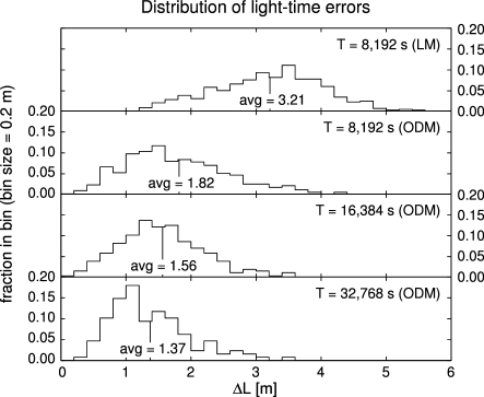
Figure 1: Distribution of errors $\Delta L$ [see Eq. (9) and the main text above it] in the determination of light travel times, using $X_{1}$-based TDIR with chunk durations of 8,192 s (for the LM and ODM models), and 16,384 and 32,768 s (for the ODM model only). As expected, the errors are lower for longer integration times $T$; for the LM model, the larger errors are due to the unmodeled curvature in the time dependence of the light-travel times. The distributions shown correspond to samples of 512, 256, and 128 chunks for $T=$ 8,192, 16,384, and 32,768 s respectively, spread across a year.

Figures 1 and 2 show the results of our simulations. The average travel-time errors $\Delta L$ displayed in Fig. 1 are defined as $\Delta L=(\Delta L_{2}+\Delta L_{2^{\prime}}+\Delta L_{3}+\Delta L_{3^{\prime}})/4$, with

$$\Delta L_{k}=\sqrt{\frac{1}{T}\int_{t_{0}}^{t_{0}+T}\left(\hat{L}_{k}(t)-L_{k}(t)\right)^{2}\,dt}.$$ (9)

Because the noises have different realizations in each chunk and because the local behavior of the $L_{k}(t)$ [Eq. (7)] changes along the year, the average error $\Delta L$ of each chunk is a random variable. Its distribution is approximated by the histograms of Fig. 1, which refer to populations of respectively 512 (for T = 8,192 s), 256 (for T = 16,384 s), and 128 (for T = 32,768 s) chunks (hence the roughness of the curves).

It turns out that the linear model is not quite sufficient to model the changes of the time-delays during the chunk lengths considered, since the minimum $\Delta L$s [computed by least-squares fitting the parameters $\hat{L}^{0}_{k}$ and $\hat{L}^{1}_{k}$ to the $L_{k}(t)$] are in the range 0.25–2.60 m (for T = 8,192 s), 1–10 m (for T = 16,384 s), and 4–40 m (for T = 32,768 s). Thus, in Figs. 1 and 2 we show results only for the linear model with T = 8,192 s. [The minimization of $I^{(n)}$ over the LM parameters is delicate, because for $X_{1}$ the laser-noise residuals turn out to depend strongly on $\Delta L_{2}$, $\Delta L_{3^{\prime}}$, and $\Delta L_{2^{\prime}}-\Delta L_{3}$, but only weakly on $\Delta L_{2^{\prime}}+\Delta L_{3}$. In this case, the Nelder–Mead algorithm can be made to return accurate results by using the search parameters $\hat{L}^{0}_{2}$, $\hat{L}^{0}_{3^{\prime}}$, $\widehat{L^{0}_{2^{\prime}}-L^{0}_{3}}$, and $\widehat{L^{0}_{2^{\prime}}+L^{0}_{3}}$, plus the corresponding $\hat{L}^{1}_{k}$ parameters.]

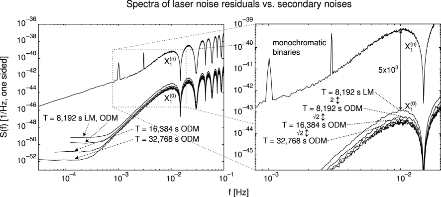
Figure 2: Spectra of frequency laser noise (bottom curves) and of GW plus secondary noises (top curve) at the end of TDIR minimization using chunk durations of 8,192 s (for the LM and ODM models), and 16,384 and 32,768 s (for the ODM model only). We show averages of the spectra computed separately for each chunk using a triangle-windowed periodogram; the averages are taken over populations of of 512, 256, and 128 chunks for $T=$ 8,192, 16,384, and 32,768 s respectively, spread across a year. In all cases, laser noise is suppressed to levels several orders of magnitude below the secondary noises: the cutout graph on the right shows that the typical laser-noise suppression factor with respect to secondary noise is $\sim 5\times 10^{3}$ for the worst case considered (8,192-s LM); it improves by a factor $\sim 2$ for 8,192-s ODM, and by factors of $\sim\sqrt{2}$ for each successive doubling of $T$. The GWs from the two circular binaries stand clearly above the noise at 1 and 3 mHz.

Figure 2 shows the spectra of the residual laser noise [i.e., of $X^{(0)}_{1}$ at the minimum of $I^{(n)}(\hat{L}_{k})$], as compared with spectra of GWs and secondary noises [i.e., of $X^{(n)}_{1}$]. The spectra are computed separately for each chunk using triangle-windowed periodograms, and then averaged over the chunk populations. The two GW sources stand clearly above the secondary noises at 1 and 3 mHz. We see that the TDI cancellation of laser noise with TDIR-determined time-delays is essentially complete, with the residual laser noise several orders of magnitude below the secondary noises. We conclude that for $T\sim 10,000$ s, with the nominal LISA noises, and even in the presence of very strong GW signals, TDIR can easily reach the time-delay accuracy required for second-generation TDI. For frequencies below 10 mHz, the residual laser-noise power decays as $f^{6}$, while the secondary noises decrease only as $f^{2}$. We attribute the flattening near 0.1 mHz (which is insignificant with respect to the LISA performance) to a combination of leakage and aliasing in the numerical estimation of the spectra and of real effects due to the first non-constant terms in the travel time errors across the chunks.

Finally, we estimate the power in the Fourier bins containing the simulated signals using two different time series: in the first $X_{1}$ was formed using perfectly known time delays, in the second using the TDIR-determined time delays. Analyzing the 32,768-s chunks at the times along the simulated year where the signal amplitudes were maximum, we find that the signal powers in the two time series agree to the numerical precision of the calculation (about a part in $10^{5}$).

In summary, we propose a method that uses TDI and the intrinsic phase noise of the lasers in a three-element array to determine the inter-spacecraft light travel times. This method, Time-Delay Interferometric Ranging (TDIR), relies on the fact that TDI nulls all the laser noises when the time delays are chosen to match the travel times experienced by the laser beams as they propagate along the sides of the array. Simulations performed using the nominal LISA noises indicate that, for integration times $\sim 10,000$ s, TDIR determines the time delays with accuracies sufficient to suppress the laser phase fluctuations to a level below the LISA secondary noises, while at the same time preserving GW signals. Our simulations assume synchronized clocks aboard the spacecraft, but we anticipate that TDIR may be extended to achieve synchronization, by minimizing noise power also with respect to clock parameters.

TDIR has the potential of simplifying the LISA design, allowing the implementation of TDI without a separate inter-spacecraft ranging subsystem. At the very least, TDIR can supplement such a subsystem, allowing the synthesis of TDI combinations during ranging dropouts or glitches. TDIR may be applicable in other forthcoming space science missions that rely on spacecraft formation flying and on inter-spacecraft ranging measurements to achieve their science objectives.

The TDIR technique presented in this paper was based on the TDI combination $X_{1}$. Since the accuracy in the estimation of the time delays achievable by TDIR depends on the magnitudes of the secondary noises entering the specific TDI combination used, it is clear that it should be possible to optimize the effectiveness of TDIR over the space of TDI combinations PTLA2002 . We will investigate this problem in a more extensive future article.

- (1) P. L. Bender, K. Danzmann, and the LISA Study Team, Laser Interferometer Space Antenna for the Detection of Gravitational Waves, Pre-Phase A Report, 2nd ed., doc. MPQ 233 (Max-Planck-Institüt für Quantenoptik, Garching, Germany, 1998).
- (2) D. A. Shaddock, M. Tinto, F. B. Estabrook, and J. W. Armstrong, Phys. Rev. D 68, 061303(R) (2003).
- (3) M. Tinto, F.B. Estabrook, and J.W. Armstrong, Phys. Rev. D 69, 082001 (2004).
- (4) M. Tinto, D. A. Shaddock, J. Sylvestre, and J. W. Armstrong, Phys. Rev. D 67, 122003 (2003).
- (5) M. Vallisneri, M. Tinto, and J. W. Armstrong, in preparation (2004).
- (6) D. A. Shaddock, B. Ware, R. E. Spero, and M. Vallisneri, Phys. Rev. D, in print (2004); gr-qc/0406106.
- (7) T. I. Laakso et al., IEEE Signal Processing Magazine 13, 30 (1996).
- (8) G. M. Jenkins and D. G. Watts, Spectral Analysis and Its Applications (Holden-Day, San Francisco, 1968).
- (9) Y. Gürsel and M. Tinto, Phys. Rev. D 40, 3884 (1989).
- (10) M. Vallisneri, gr-qc/0407102.
- (11) N. Cornish and L. Rubbo, Phys. Rev. D 67, 022001 (2003).
- (12) W. Folkner, private communication (2004).
- (13) J. A. Nelder and R. Mead, Computer Journal 7, 308 (1965).
- (14) T. A. Prince, M. Tinto, S. L. Larson, and J. W. Armstrong, Phys. Rev. D 66, 122002 (2002).