Quantum cosmology and the accelerated Universe

In order to explain the present accelerated expansion of the Universe, suggested by the measurements of high redshifts supernovae[2] [3], we consider that presently, at cosmological scales, classical General Relativity (GR) is not valid. Instead of changing the right hand side of Einstein’s equations by introducing some new negative pressure fluid, we modify its left hand side according to physical considerations. We study a quantum universe and, keeping in mind that a macroscopic universe behaves classicaly or quantically depending on its initial quantum state, we investigate if is it possible that quantum cosmological effects at large scales can mimic a negative pressure fluid yielding a positive acceleration. The aim of this talk is to show with a simple model that it is indeed possible for some suitable initial quantum states of the universe. We consider a quantum minisuperspace model containing a free massless scalar field $\phi$ minimally coupled to gravity in a Friedmann geometry. We interpret this model in the framework of the Bohm-de Broglie (BdB) interpretation of quantum theories [4] [5], in order to extract predictions from the wave functional of the Universe. After quantize the model according to Dirac’s procedure, we obtain the Wheeler-DeWitt (WDW) equation. We only concentrate in the flat model and we consider the following solution of WDW equation $\Psi=\mid\sigma\mid\sqrt{\pi}\{\exp{[-\frac{(\alpha+\phi)^{2}\sigma^{2}}{4}]}\exp(id(\alpha+\phi))+\exp{[-\frac{(\alpha-\phi)^{2}\sigma^{2}}{4}]}\exp(id(\alpha-\phi))\}$, where $\alpha\equiv\ln(a)$ being $a$ the (dimensionless) scale factor and $\sigma$ and $d$ are parameters of the quantum model[1]. The quantum trajectories, can be obtained by integrating the Bohm’s guidance equations, given by: $\dot{\alpha}=\frac{\phi\sigma^{2}\sin(2d\phi)-2d\cos(2d\phi)-2d\cosh(\sigma^{2}\alpha\phi)}{e^{3\alpha}2[\cos(2d\phi)+\cosh(\sigma^{2}\alpha\phi)]}$ and $\dot{\phi}=-\frac{\alpha\sigma^{2}\sin(2d\phi)+2d\sinh(\sigma^{2}\alpha\phi)}{e^{3\alpha}2[\cos(2d\phi)+\cosh(\sigma^{2}\alpha\phi)]}$. They are shown in Fig. 1. We can see two different possibilities. Oscillating universes without singularities around the centers points and non-oscillating universes. A non oscillating universe arises classically from a singularity, experiences quantum effects in the middle of its expansion, and recover its classical behaviour for large values of $\alpha$. The quantum effects appearing in the middle of the expansion can deviate it from its classical decelerated expansion to an accelerated one. We can see that this is indeed the case for this model, by plotting the acceleration $\frac{\ddot{a}}{a}$ as a function of $\alpha$ and $\phi$ : $\frac{\ddot{a}}{a}=E(\alpha,\phi)$ (Fig. 2). We can see regions on the plane $\alpha$-$\phi$ where the acceleration is positive, negative or zero. One can see the classical behaviour $\ddot{a}/a\propto-1/a^{6}$ for $a\rightarrow 0$ ($\alpha\rightarrow-\infty$) and $a\rightarrow\infty$ ($\alpha\rightarrow\infty$), but near the region $a=1$ ($\alpha=0$), a clear departure from classical behaviour is observed, and positive values of $\ddot{a}/a$ are obtained. We can compare the quantum cosmological model with the original classical free scalar field model, classically equivalent to stiff matter, with flat spatial section, suplemented with a cosmological constant as an alternative source for accelerated expansion. It is possible to show that for the quantum model we have $-0.21<q_{0}<-0.17$ for $2d\phi_{0}=2n\pi+x$ with $x\in(2.145,2.15)$, provided a very large value for $\sigma$[1]. Note that, for the classical model with $\Omega_{\Lambda}=0.73$, $q_{0}=-0.19$. The supernovae measurements relate the luminosity distance $d_{L}$ with $z$. Hence, it would be instructive to compare the quantum cosmological luminosity distance $d_{L}^{q}(z)=(1+z)\int_{0}^{z}\frac{{\rm d}y}{\dot{\alpha}(y)}$, with the classical one. In Fig.3, we show a plot of $H_{0}d_{L}(z)$ with $\Omega_{\Lambda}=0.73$ , $H_{0}d_{L}(z)$ with $\Omega_{\Lambda}=0$, and $H_{0}d_{L}^{q}(z)$. Note that for small values of $z$ they are close but, for intermediary values of $z$, the quantum $d_{L}^{q}(z)$ remain close to the cosmological constant $d_{L}(z)$ while both separates of the pure stiff matter $d_{L}(z)$. Hence, quantum cosmological effects may mimic a cosmological constant in some region but not everywhere. In this way, it may be possible to explain the positive acceleration suggested by the recent measurements of high redshift supernovae without postulating a new contribution to the energy density of the Universe as the dark energy. Of course, more elaborated models including matter sources like dust and radiation must be studied.

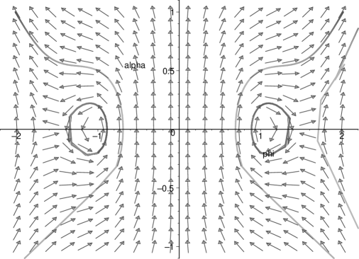
Figure 1: Field plot of the system of planar equations (the guidance equations), giving the quantum trajectories. For numerical simplicity we choose the values $-d=\sigma=1$.

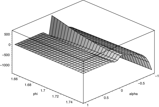
Figure 2: Acceleration $\ddot{a}/a$ as a function of $\phi$ and $\alpha$. For numerical simplicity we choose the values $-d=\sigma=1$.

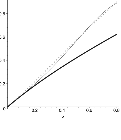
Figure 3: The luminosity distance as a function of redshift. The thin line curve corresponds to the quantum model, the dotted curve is for the classical model with a cosmological constant, and the thick line curve is for the classical model without cosmological constant.

References

- [1] N. Pinto-Neto and E. Sergio Santini, Phys. Lett. A 315:36-50 (2003).
- [2] Perlmutter, S. et al., The Astronomical Journal, 116:1009-1038 (1998); Nature (London) 391, 51 (1998) and The Astrophysical Journal, 517: 565-586 (1999).
- [3] A. Riess et al., Astron. J. 116, 1009, (1998).
- [4] David Bohm, Phys. Rev. 85, 166 and 180 (1952).
- [5] P. R. Holland, The Quantum Theory of Motion: An Account of the de Broglie-Bohm Causal Interpretation of Quantum Mechanics (Cambridge University Press, Cambridge, 1993).
- [6] R. Colistete Jr., J. C. Fabris and N. Pinto-Neto, Phys. Rev. D62, 83507 (2000).
- [7] N. Pinto-Neto and E. Sergio Santini, Phys.Rev. D 59 123517 (1999).
- [8] N. Pinto-Neto and E. Sergio Santini, Gen. Rel. and Grav. 34, 505 (2002).
- [9] E. Sergio Santini, PhD Thesis, CBPF-Rio de Janeiro, (May 2000), (gr-qc/0005092).