Electromagnetic Magic: The Relativistically Rotating Disk

Abstract

A closed form analytic solution is found for the electromagnetic field of the charged uniformly rotating conducting disk for all values of the tip speed $v$ up to $c$. For $v=c$ it becomes the Magic field of the Kerr-Newman black hole with $G$ set to zero.

The field energy, field angular momentum and gyromagnetic ratio are calculated and compared with those of the electron.

A new mathematical expression that sums products of 3 Legendre functions each of a different argument, is demonstrated.

I Introduction

Away from sources we write the electromagnetic field ${\bf{F}}={\bf{E}}+i{\bf{B}}=-\nabla\Psi$ where $\Psi=\Phi+i\raisebox{1.99997pt}{$\chi$}$ is a complex potential satisfying $\nabla^{2}\Psi=0$. The simplest solution is the real one $\Psi=q/r$ but if we make $q$ complex we introduce a magnetic monopole which is unacceptable. Moving the charge to $\tilde{\bf{a}}$ we have a potential $q/\sqrt{(\bf{r-\tilde{a}})^{2}}$ which corresponds to a charge at $\tilde{\bf{a}}$ when $\tilde{\bf{a}}$ is real, but we now consider $\tilde{\bf{a}}$ to be complex ${\bf{r}}_{1}+i\bf{a}$. Without loss of generality we may move the origin to $\bf{r}_{1}$ and orient the $z$ axis along $\bf{a}$. If we then set $z=r\cos\theta=r\mu$ we find

$$\Psi=q/\sqrt{({\bf{r}}-i{\bf{a}})^{2}} = q/(r^{2}-2iar\mu-a^{2})^{1/2}$$

$$= \frac{q}{r}\sum\left(\frac{ia}{r}\right)^{n}P_{n}(\mu)~{}~{}{\rm for}~{}r\geqslant a~{}.$$

$\Psi$ has a singular ring at $\mu=0$ and $r=a$. To specify $\Psi$ properly we need to say which square root is to be taken, but the expansion above for $r\geqslant a$ is required to make everything regular at infinity and the simplest cut is across the circle defined by the ring singularity. With such a cut analytic continuation defines $\Psi$ everywhere. The ‘magic’ field is given by

$${\bf{F=E}}+i{\bf{B}}=-\nabla\Psi=q\frac{{\bf{r}}-i{\bf{a}}}{[({\bf{r}}-i{\bf{a}})^{2}]^{3/2}}$$ (2)

By construction $\nabla^{2}\Psi=0$ except on the singular ring and the cut, so the sources of the field lie there. The expansion (I) shows that the field has charge $q$, no magnetic monopole but a magnetic dipole $qa$. Indeed the electric field has only even multipoles and the magnetic field has only odd ones. On $z=0,~{}{\bf{a.r}}=0$ so the denominator of (2) is real if $r\geqslant a$ and pure imaginary for $r<a$.

Thus close to the plane of symmetry

$${\bf{E}}=-q{\bf{a}}/(a^{2}-r^{2})^{3/2}~{},$$

and ${\bf{B}}=-q{\bf{r}}/(a^{2}-r^{2})^{3/2}$ for $z>0$ and $r<a$. Below, where $z<0$ these fields are reversed. Notice that $\bf{E}$ is orthogonal to the disk so the disk is an equipotential and indeed its potential is zero (earthed) as may be seen by taking the real part of (I) on $z=0$ with $r^{2}<a^{2}$. The magnetic field lies parallel to the radius below the disk and anti-parallel above. It does not cross the disk except at the singular ring. For $r>a$ and $z=0$, $\bf{B}$ points downwards everywhere. Thus every field line returns to the upper hemisphere through the singular ring.

From the electric field one readily calculates the surface density of charge on the disk (summing both sides)

$$\sigma=-\frac{qa}{2\pi(a^{2}-r^{2})^{3/2}}$$ (3)

Notice that this is of the opposite sign to the total $q$ which is rectified only at the singular ring. Indeed the total charge on the cut within $r=R$ is $Q(<R)=-q\left(\frac{a-\sqrt{a^{2}-R^{2}}}{\sqrt{a^{2}-R^{2}}}\right)$ for $R<a$ which diverges with a negative sign as $R$ approaches $a$ but $Q(<R)=+q$ for $R>a$ so the negative infinity is now replaced by a finite positive result. Likewise the surface current in the cut is

$$J_{\phi}=-\frac{q}{2\pi}~{}\frac{r}{(a^{2}-r^{2})^{3/2}}$$ (4)

which is precisely what we would get if the above charge density were rotating rigidly with angular velocity $\Omega=c/a$. The total current within $R<a$ is $Q(<R)\Omega/(2\pi c)$. Again the magnetic effects of this current are overwhelmed by the current around the singular ring which is of opposite sign. Notice that the disk is not crossed by a magnetic field line saving at the singular edge ring itself. In this respect the disk acts like a superconductor displaying the Meissner effect. In the Black Hole context this phenomenon was noted by Bic̆ák & Janis̆ [1] (see also Bic̆ák & Ledvinka [2]).

I now list other properties of this ‘Magic’ electromagnetic field. (For proofs see Lynden-Bell [3])

1. Relativistic Invariants $F^{2}=E^{2}-B^{2}+2i{\bf{E.B}}=q^{2}/({\bf{r}}-i{\bf{a}})^{4}$.

2. $E^{2}=B^{2}$ only on two spheres of radius $\sqrt{2}a$ centred on ${\bf{r}}=\pm{\bf{a}}$. They meet on the singular ring.

3. ${\bf{E.B}}=0$ on the sphere $r=a$ and also on the plane $z=0$.

4. The field energy density ${\bf{F.F^{*}}}/8\pi=[q^{2}/(8\pi)](r^{2}+a^{2})/|({\bf{r}}-i{\bf{a}})^{2}|^{3}$. This diverges like $(r-a)^{-3}$ when $z=0$ near $r=a$.

5. ${\bf{F^{*}}}\times{\bf{F}}=2iq{\bf{E}}\times{\bf{B}}=2iq^{2}{\bf{a}}\times{\bf{r}}/|({\bf{r}}-i{\bf{a}})^{2}|^{3}$ likewise diverges.

6. The above is related to the Poynting vector which shows that the energy density flows around the axis with a velocity $\bm{\Omega}\times{\bf{r}}$ where $\bm{\Omega}$ is constant on spheres $r=$const with $\bm{\Omega}(r)=\frac{2{\bf{a}}c}{r^{2}+a^{2}}$.

7. Landau & Lifshitz [4] show that in the frame that moves with the velocity $c{\bf{V}}$ where ${\bf{V}}/(1+V^{2})={\bf{E}}\times{\bf{B}}/(E^{2}+B^{2})$, the transformed fields ${\bf{E}}^{\prime}\&{\bf{B}}^{\prime}$ are parallel. Gair proved the theorem that these velocities are a uniform rotation of each spheroid confocal with the disk at the rate $\bm{\Omega}={\bf{a}}c/(\tilde{r}^{2}+a^{2})$ (for $\tilde{r}$ see section 2).

8. In the corotating frame of those spheroids ${\bf{E}}^{\prime}$ and ${\bf{B}}^{\prime}$ are both perpendicular to the spheroid on which they lie.

9. The total field energy and the total angular momentum in the field both diverge due to their divergence at the singular ring.

More remarkable properties still come from the separability of both wave equations and equations of motion of any relativistic charged particle in this field.

1. The Hamilton-Jacobi equation separates

2. The Klein Gordon equation separates

3. The Dirac equation separates

4. The Schrödinger equation separates if only the real part of the field is included (but not when the magnetic part is added although the reverse is true for the Klein Gordon equation).

All the above really stem from remarkable investigations in the separability of wave equations around black holes by Carter [5],[6], Teukolsky [7], Chandrasekhar [8] and Page [9]. In the simpler flat space case see Lynden-Bell Paper I [10].

Finally the relationship with black holes and indeed the original discovery of the field in General Relativity is due to Newman et al. [11] who generalised the Kerr metric of a spinning black hole to include charge. If in his solution one puts Newton’s $G\equiv 0$ one obtains an electromagnetic field in flat space which is the above ‘Magic’ field [12], [13], [14].

The present investigation is aimed at providing a set of electromagnetic fields in flat space that keep some of the remarkable properties of the Magic field but give finite answers for total field energy, total field angular momentum etc. We aim to find fields which give the Magic field as a limiting case but whose other members give finite answers. Some spice is added to the investigation by Carter’s [5] remark that all Kerr Metrics have the same gyromagnetic ratio, 2, as the Dirac electron, and Pfister & King [15] propose that this may have a deeper significance for general relativity. Indeed it holds for all the conformastationary metrics, the statement by us [16] that the gyromagnetic ratio was one, was based on erroneously missing out the factor 2 in its definition. Our disk [16] remains the only known conformastationary interior solution to Einstein’s equation.

Recently [17] we discussed the remarkable behaviour of charges on a relativistically rotating conducting sphere. The changes in the field correspond to addition of more and more of the Magic field as the rotation increases. However even when $v=c$ the distribution on the sphere never becomes the Magic field: that discussion leads to the suggestion that the Magic field may be the field of the rapidly rotating charged conducting plate with a tip speed of $c$. The facts that the component of ${\bf{E}}+{\bf{V}}\times{\bf{B}}$ in the plate is zero and that the current is due to the convected charge strongly suggest that this is the limit, as $Vc$ the tip speed tends to $c$, of the charged rotating conducting plate. This paper is devoted to a discussion of the whole sequence of fields of such a plate when it rotates at any tipspeed up to $c$. The field lines of the Magic field are shown in Figure 1, which was generated by J. Gair.

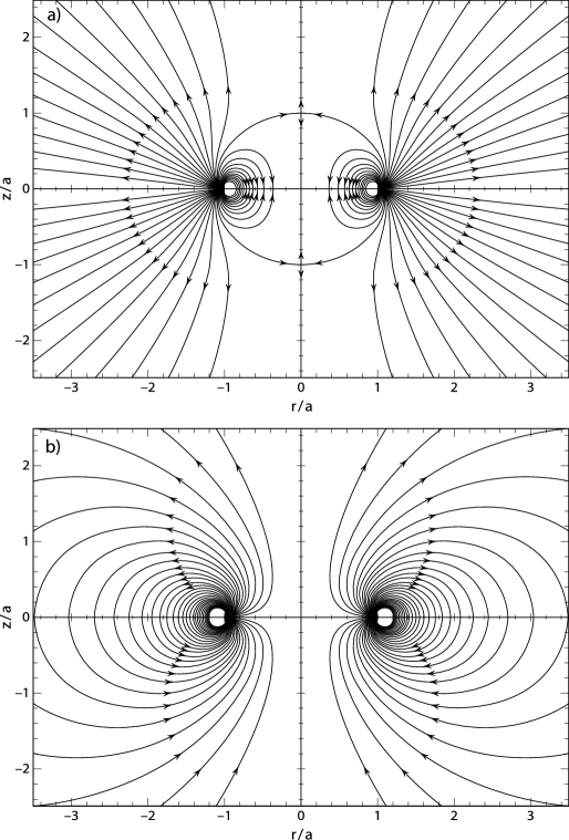
Figure 1: (a) Electric lines of force for the Kerr-Newman potential. The density of lines reflects the strength of the field.
(b) Magnetic lines of force for the Kerr-Newman potential. The density of lines reflects the strength of the field.

II Maxwell’s Equations for the Rotating Disk

We treat the problem using oblate spheroidal coordinates confocal with the ring that forms the edge of the disk. Actually we shall solve the problem as the limit of a highly flattened spheroid as its minor axis $\tilde{b}$ tends to zero; this allows us to make direct comparisons with our treatment of the rotating charged conducting sphere. The equation

$$\frac{x^{2}+y^{2}}{\tau+a^{2}}+\frac{z^{2}}{\tau}=1$$ (5)

defines a set of confocal oblate spheroids each with a definite positive value of $\tau$. When $\tau=0$ it defines a disk $z=0,~{}x^{2}+y^{2}\leqslant a^{2}$. When $\tau$ is negative it defines a set of hyperboloids of revolution (of one sheet) each of which is orthogonal to the oblate spheroids. For $\tau$ positive we write it as $\tilde{r}^{2}$ and for $\tau$ negative we write it as $-a^{2}\cos^{2}\vartheta$ or more often as $-a^{2}\tilde{\mu}^{2}$. The spheroidal coordinates $\tilde{r},\vartheta$ are supplemented by the usual azimuthal angle $\phi$ to give the metric

$$ds^{2} = \frac{\tilde{r}^{2}+a^{2}\tilde{\mu}^{2}}{\tilde{r}^{2}+a^{2}}d\tilde{r}^{2}+\frac{(\tilde{r}^{2}+a^{2}\tilde{\mu}^{2})}{1-\tilde{\mu}^{2}}d\bar{\mu}^{2}$$

$$+ (1-\tilde{\mu}^{2})(\tilde{r}^{2}+a^{2})d\phi^{2}$$

$$= dr^{2}+r^{2}d\theta^{2}+r^{2}\sin^{2}\theta d\phi^{2}$$

$$= dR^{2}+R^{2}d\phi^{2}+dz^{2}$$

where $\theta$ is the spherical polar coordinate which should be distinguished from the spheroidal coordinate $\vartheta$ although they are equal at $\infty$. We consider the surface of the spheroid $\tilde{r}=\tilde{b}$ to be the rotating conductor.

On $\tilde{r}=0$, the disk, $\partial\raisebox{1.99997pt}{$\chi$}/\partial\tilde{r}$ changes sign which corresponds to the continuity of the normal magnetic flux, and $\Phi$ is continuous which corresponds to the surface component of the electric field being continuous.

The other requirements are that the total charge must be $q$, so $\Phi\rightarrow q/r$ at $\infty$ and ${\bf{E}}+\frac{1}{c}(\bm{\Omega}\times{\bf{r}})\times{\bf{B}}$ must have no component along the disk’s surface so that the Lorentz force component vanishes. Of course the discontinuity of the surface component of $-\nabla\raisebox{1.99997pt}{$\chi$}$ corresponds to the surface current $4\pi J_{\phi}$ and the discontinuity in the normal component of $-\nabla\Phi$ gives the surface density of charge $4\pi\sigma$. In the steady state with an imperfect conductor the currents are just those caused by the rotation of the charge.

$${\bf{J}}=\frac{1}{c}(\bm{\Omega}\times{\bf{r}})\sigma$$ (7)

That completes the physical specification of the problem. Now we turn these physical requirements into mathematics.

On the disk

$$\mathcal{I}m(-\partial\Psi/\partial R) = B_{R}=2\pi J_{\phi}$$

$$\mathcal{R}e(-\partial\Psi/\partial z) = 2\pi\sigma$$

and from the Lorentz force component

$$\mathcal{R}e(-\partial\Psi/\partial R)+(\Omega R/c)\mathcal{I}m(-\partial\Psi/\partial z)=0$$

while (7) gives

$$\mathcal{I}m(-\partial\Psi/\partial R)-(\Omega R/c)\mathcal{R}e(-\partial\Psi/\partial z)=0$$

Hence on the disk $R<a$, $z=0$

$$\partial\Psi/\partial R=i(\Omega R/c)\partial\Psi/\partial z$$ (8)

Now in spheroidal coordinates the general solution of Laplace’s equation which tends to $q/r$ at $\infty$ is

$$\Psi=\frac{q}{ia}\sum^{\infty}_{0}\Psi_{l}~{}P_{l}(\tilde{\mu})Q_{l}\left(\frac{\tilde{r}}{ia}\right)$$ (9)

$P_{l}(\tilde{\mu})$ are the Legendre Polynomicals and the $Q_{l}\left(\frac{\tilde{r}}{ia}\right)$ are the Legendre functions here expressed as functions of an imaginary argument. The $Q_{2l}\left(\frac{\tilde{r}}{ia}\right)$ are imaginary while the $Q_{2l+1}\left(\frac{\tilde{r}}{ia}\right)$ are real. The $Q_{l}(z)$ obey the recurrence relations $(l+1)Q_{l+1}(z)=(2l+1)zQ_{l}(z)-lQ_{l-1}(z)$ and $(z^{2}-1)Q_{l}^{\prime}(z)=lzQ_{l}(z)-lQ_{l-1}(z)$.

Hereafter whenever we refer to $Q_{l}$ or $Q_{l}^{\prime}$ without explicit mention of its argument we shall mean $Q_{l}(0)$ and $Q_{l}^{\prime}(0)$ i.e. the limit of $Q_{l}\left(\frac{\tilde{b}}{ia}\right)$ as $\tilde{b}\rightarrow 0$ etc. We then have

$$Q_{l-1}=-[(l+1)/l]Q_{l+1}~{}~{}{\rm and}~{}~{}Q_{l}^{\prime}=lQ_{l-1}=-(l+1)Q_{l+1}$$ (10)

$$Q_{0}(z)=\frac{1}{2}\ln\left(\frac{z-1}{z+1}\right) \rightarrow -\frac{i\pi}{2}~{}~{}{\rm as}~{}~{}z\rightarrow\frac{b}{ia}\rightarrow 0$$

$$\rightarrow ia/\tilde{r}~{}~{}{\rm as}~{}~{}z=\frac{\tilde{r}}{ia}\rightarrow\infty$$

$$Q_{1}(z)=\frac{z}{2}\ln\left(\frac{z+1}{z-1}\right)-1 \rightarrow -1~{}~{}{\rm as}~{}~{}z\rightarrow 0$$

The condition that $\Psi\rightarrow q/r$ at $\infty$ becomes $\Psi_{0}=1$. Rewriting our boundary condition (8) in spheroidal coordinates

$$-\frac{\sqrt{1-\tilde{\mu}^{2}}}{a|\tilde{\mu}|}~{}\frac{\partial\Psi}{\partial\tilde{\mu}}=\frac{i\Omega a}{c}~{}\frac{\sqrt{1-\tilde{\mu}^{2}}}{|\tilde{\mu}|}~{}\frac{\partial\Psi}{\partial\tilde{r}}~{}~{}~{}{\rm on}~{}~{}\tilde{r}=0$$

Thus from (9) setting $\Omega a/c=\omega$

$$\sum^{\infty}_{0}\Psi_{l}~{}P_{l}^{\prime}(\tilde{\mu})Q_{l}=-\omega\sum^{\infty}_{0}\Psi_{l}P_{l}(\tilde{\mu})Q^{\prime}_{l}$$ (11)

Now as well as their usual orthogonality relation the Legendre polynomicals $P_{l}(\mu)$ have the property

$$\int^{+1}_{-1}\!P^{\prime}_{l+1}(\mu)~{}P_{m}(\mu)~{}d\mu=\begin{cases}2~{}{\rm for}~{}l\geqslant m,~{}(l+m)~{}{\rm even}\\ 0~{}{\rm for}~{}l<m~{}{\rm or}~{}(l+m)~{}{\rm odd}\end{cases}$$

Multiplying (11) by $\frac{1}{2}P_{2m}(\tilde{\mu})$ and integrating $-1$ to $+1$

$$\sum^{\infty}_{m}(4l+3)\eta_{2l+1}~{}Q_{2l+1}=-\omega\eta_{2m}~{}Q^{\prime}_{2m}=-\omega\eta_{2m}2mQ_{2m-1}$$ (12)

where $\eta_{m}=\Psi_{m}/(2m+1)$. Subtracting this with $(m+1)$ written for $m$

$$(4m+3)\eta_{2m+1}Q_{2m+1} = \omega[\eta_{2m+2}(2m+2)Q_{2m+1}$$

$$+ \eta_{2m}(2m+1)Q_{2m+1}]$$

where we used (10) on the last term. Thus

$$(4m+3)\eta_{2m+1}=\omega\left[(2m+2)\eta_{2m+2}+(2m+1)\eta_{2m}\right]$$ (13)

similarly multiplying (11) by $\frac{1}{2}P_{2m+1}(\tilde{\mu})$ and integrating etc

$$(4m+5)\eta_{2m+2}=\omega\left[(2m+3)\eta_{2m+3}+(2m+2)\eta_{2m+1}\right]$$ (14)

(13) & (14) can be recombined into a single formula true for all $m$

$$(2m+1)\eta_{m}=\omega\left[(m+1)\eta_{m+1}+m\eta_{m-1}\right]~{}.$$ (15)

When the Magic potential is rewritten in terms of the spheroidal coordinates $\tilde{r}$ and $\tilde{\mu}$ it takes a remarkably simple form and it is interesting to resolve it into Legendre polynomials of $\tilde{\mu}$

$$\Psi = q/\sqrt{({\bf{r}}-i{\bf{a}})^{2}}=q/(\tilde{r}-ia\tilde{\mu})$$

$$= \left(\frac{q}{ia}\right)\sum^{\infty}_{0}M_{l}\left(\frac{\tilde{r}}{ia}\right)P_{l}(\tilde{\mu})$$

We multiply both sides by $P_{n}(\tilde{\mu})$ and integrate $-1$ to $+1$. By Abramowitz & Stegan 8.8.3 $\frac{1}{2}\int^{+1}_{-1}\frac{P_{n}(\mu)}{(z-\mu)}d\mu=Q_{n}(z)$ so we find $M_{l}\left(\frac{\tilde{r}}{ia}\right)=(2l+1)Q_{l}\left(\frac{\tilde{r}}{ia}\right)$ and in terms of the expansion (9) $\Psi_{l}=2l+1$ so $\eta_{l}=1$ for the Magic field. We see at once that this satisfies (15) with $\omega$ set equal to 1 so that the Magic field is as expected the limit of the uniformly rotating disk when $v\rightarrow c$. To solve our problem for a general rotation rate we use the generating function method developed in the appendix of Paper III [17].

We multiply equation (15) by $U^{m}$ and sum from $m=1$ to $\infty$. Defining $\eta(U)=\sum\limits^{\infty}_{0}\eta_{m}U^{m}$ and remembering that $\eta_{0}=\Phi_{0}=1$ we find that

$$2U\eta^{\prime}+\eta-1=\omega(\eta^{\prime}-\eta_{1}+U^{2}\eta^{\prime}+\eta)$$

We rewrite this in terms of the roots $u\leqslant 1$ and $1/u$ of the quadratic $t^{2}-\frac{2}{\omega}t+1=0$ so $\frac{1}{\omega}=\frac{1}{2}(u^{-1}+u)$. [Notice that the quadratic and $u$ differ from those of paper III in which we discussed the sphere rather than the disk]

$$(U-u)(U-u^{-1})\eta^{\prime}+[U-\frac{1}{2}(u^{-1}+u)]\eta=\eta_{1}-\frac{1}{\omega}$$ (16)

The general solution for the generating function $\eta(U)$ is

$$\eta=I^{-1}[(\eta_{1}-\frac{1}{\omega})\int^{U}_{0}I^{-1}dU+C]$$ (17)

where $I$, the integrating factor, is given for $U\leqslant u$ by

$$I=[(U-u)(U-u^{-1})^{1/2}=[1-\frac{2}{\omega}U+U^{2}]^{1/2}~{}.$$ (18)

In general the expression (17) has a factor behaving like $(u-U)^{-1/2}$ which diverges at $U=u$. Its expansion as a power series is of the form $u^{-1/2}\left(1+\frac{1}{2}u^{-1}U...+\frac{1/2~{}3/2...\frac{2n-1}{2}}{n!}(u^{-1}U)^{n}+...\right)$ which gives rise to terms in $u^{-(n+1/2)}$ which diverge as $n$ becomes large because $u<1$. To suppress this divergence we must choose the constant

$$C=-\left(\eta_{1}-\frac{1}{\omega}\right)\int^{u}_{0}I^{-1}dU~{}.$$

Then the numerator vanishes at $U=u$ and

$$\eta=-\left(\eta_{1}-\frac{1}{\omega}\right)I^{-1}\int^{u}_{U}I^{-1}dU$$

But $\eta_{0}=\eta(0)=1$ so $\eta_{1}=\frac{1}{\omega}-[\int^{u}_{0}I^{-1}dU]^{-1}$.

Now $I^{2}=\left[U-\frac{1}{2}(u^{-1}+u)\right]^{2}-\left[\frac{1}{2}(u^{-1}-u)\right]^{2}$ and $I(0)=1$, so we set $\frac{1}{2}(u^{-1}+u)-U=\frac{1}{2}(u^{-1}-u)ch~{}w$; then $I=\frac{1}{2}(u^{-1}-u)sh~{}w$ and $w=0$ when $U=u$. Also

$$\int^{u}_{U}I^{-1}dU=w~{}.$$

Hence

$$\eta(U)=-\left[\frac{\eta_{1}-\frac{1}{2}(u^{-1}+u)}{\frac{1}{2}(u^{-1}-u)}\right]~{}\frac{w}{shw}$$ (19)

and

$$\eta(0)=\left(\frac{1}{\omega}-\eta_{1}\right)ch^{-1}\gamma$$ (20)

where $\gamma^{-2}=1-\omega^{2}=1-v^{2}/c^{2}~{};~{}\gamma=\frac{u^{2}+1}{u^{2}-1}$. But $\eta(0)=\eta_{0}=1$ so we have

$$\eta_{1}=1/\omega-1/ch^{-1}\gamma\rightarrow 1~{}{\rm as}~{}\omega\rightarrow 1~{}.$$ (21)

Thus at $\omega=1$ our recurrence relation (15) yields the Magic field with $\eta_{n}=1$ all $n$. We now know both $\eta_{0}=1$ and $\eta_{1}(\omega)$ as a function of $\omega$; thus we are now in a position to use our recurrence relation to generate all the $\eta_{m}$ for any chosen value of $\omega$. Alternatively we could expand our expression for $\eta(U)$ as a power series in $U$ and pick out the coefficient of $U^{m}$. However Prof J.F. Harper pointed out to me that the recurrence relation (15) is that obeyed by the Legendre Polynomials $P_{n}\left(\frac{1}{\omega}\right)$. Notice that $\frac{1}{\omega}$ is greater than 1. Since the $P_{n}$ and the $Q_{n}$ obey the same recurrence relation the general solution is a linear combination of them. Fitting that combination to $\eta_{0}=1$ and the value of $\eta_{1}$ just derived we find, noting that $ch^{-1}\gamma\equiv Q_{0}\left(\frac{1}{\omega}\right)$,

$$\eta_{n}=Q_{n}\left(\frac{1}{\omega}\right)/Q_{0}\left(\frac{1}{\omega}\right)~{}.$$ (22)

Thus the solution for the complex potential is

$$\Psi=\frac{q}{ia}\sum(2n+1)\!\left[Q_{n}\!\left(\frac{1}{\omega}\right)\!/Q_{0}\!\left(\frac{1}{\omega}\right)\!\right]\!Q_{n}\!\left(\frac{\tilde{r}}{ia}\right)\!P_{n}(\tilde{\mu})~{}.$$ (23)

We note that $Q_{n}\left(\frac{1}{\omega}\right)/Q_{0}\left(\frac{1}{\omega}\right)\rightarrow 1$ as $\omega\rightarrow 1$ so the Magic field is still there in that limit. Now by [18] 8.8.2 $Q_{n}(z)\rightarrow z^{-n-1}\int^{\infty}_{0}(1+cht)^{-n-1}dt$ as $z\rightarrow\infty$. Hence

$$Q_{n}\left(\frac{1}{\omega}\right)/Q_{0}\left(\frac{1}{\omega}\right) \rightarrow \omega^{n}\int^{\infty}_{1}\frac{2^{n+1}x^{n}}{(1+x)^{2n+2}}dx$$

$$= \begin{cases}\omega^{n}2^{n}(n!)^{2}/(2n+1)!\\ \qquad+0(w^{n+2})\end{cases}$$

so for small $\omega$

$$\Psi=\frac{q}{ia}\sum\frac{2^{n}(n!)^{2}}{(2n)!}\omega^{n}Q_{n}\left(\frac{\tilde{r}}{ia}\right)P_{n}(\bar{\mu})~{}.$$ (24)

Now

$$Q_{0}\left(\frac{\tilde{r}}{ia}\right) = \ln\sqrt{\frac{\tilde{r}+ia}{\tilde{r}-ia}}=i~{}\tan^{-1}\left(\frac{a}{\tilde{r}}\right)$$

$$Q_{1}\left(\frac{\tilde{r}}{ia}\right) = \frac{\tilde{r}}{a}\tan^{-1}\frac{a}{\tilde{r}}-1~{};$$

$$Q_{2}\left(\frac{\tilde{r}}{ia}\right) = \left(\frac{-3\tilde{r}^{2}/a^{2}-1}{2}\right)i~{}tan^{-1}\left(\frac{a}{\tilde{r}}\right)+\frac{i3\tilde{r}}{2a}$$

so

$$\Psi = \frac{q}{a}\left\{\tan^{-1}\frac{a}{\tilde{r}}+i\omega\left[1-\frac{\tilde{r}}{a}\tan^{-1}\left(\frac{a}{\tilde{r}}\right)\right]\tilde{\mu}\right.$$ (25)

$$+ \left.\omega^{2}\left[\frac{\tilde{r}}{a}-\left(\left(\frac{\tilde{r}}{a}\right)^{2}+3\right)\tan^{-1}\frac{a}{\tilde{r}}\right]P_{2}(\tilde{\mu})\right.$$

$$+ \left.O(\omega^{3})\right\}$$

The first term is the well known potential of a static charged disk.

We may now read off expressions for the charge $q$, the (magnetic) dipole moment $\mu_{m}$ and the (electric) quadrupole moment $Q_{e}$

$$\mu_{m}=qa\left(\frac{1}{\omega}-\frac{1}{\lambda}\right)\rightarrow\begin{cases}\frac{1}{3}qa\omega+O(\omega^{2})\\ qa~{};~{}\omega\rightarrow 1\end{cases}$$

where we have defined $\lambda=\ln\sqrt{\frac{1+\omega}{1-\omega}}=ch^{-1}\gamma$.

In finding the quadrupole moment for $\omega$ small we note that part of it comes from the oblateness of the $\tilde{r}=$const surfaces. Taking the sign so an oblate distribution has negative $Q$

$$Q_{e}=-\frac{1}{3}qa^{2}\!\left[1+2Q_{2}\left(\frac{1}{\omega}\right)/\lambda\right]\!\rightarrow\!\begin{cases}-\frac{1}{3}qa^{2}\left(1+\frac{4}{5}\omega^{2}\right)\\ -qa^{2}~{};~{}\omega\rightarrow 1\end{cases}\!\!.$$

III Closed Form Exact Potential

On the axis $\tilde{\mu}=1$, so all the $P_{n}(\bar{\mu})=1$ and we can then perform the summation (23) using a result in Whittaker & Watson [19]

$$\sum(2n + 1)Q_{n}\left(\frac{1}{\omega}\right)Q_{n}\left(\frac{\tilde{r}}{ia}\right)$$

$$= \frac{1}{2\left(\frac{\tilde{r}}{ia}-\frac{1}{\omega}\right)}\ln\left[\frac{1+\omega}{1-\omega}.\frac{\tilde{r}-ia}{\tilde{r}+ia}\right]$$

On the axis $\tilde{r}=z$ so we obtain the complex potential setting $b=\frac{a}{\omega}$

$$\Psi(z)=\frac{q}{z-ib}\left[1+\frac{1}{2\lambda}\ln\left(\frac{z-ia}{z+ia}\right)\right]~{}.$$ (26)

Now there is a remarkable way [20] of obtaining the solution of $\nabla^{2}\Psi=0$ everywhere if it is given as an analytic function $\Psi(z)$ on the axis. The potential everywhere is given by (see Appendix A)

$$\Psi(R,z)=\frac{1}{2\pi}\int^{2\pi}_{0}\Psi(z+iR\cos\alpha)d\alpha~{}.$$

In our application it is simplest to use $\tan\frac{\alpha}{2}=t$ as the variable of integration. The solution is then

$$\Psi(R,z)=\frac{1}{\pi}\int^{\infty}_{-\infty}\Psi\left(z+iR\frac{1-t^{2}}{1+t^{2}}\right)\frac{dt}{1+t^{2}}$$

applied to the $\Psi(z)$ given by (26) we find

$$\Psi(R,z)=\frac{1}{\pi}\int^{\infty}_{-\infty}\frac{q}{(z-ib+iR)+(z-ib-iR)t^{2}}$$

$$\left\{1+\frac{1}{2\lambda}\ln\left[\frac{(z-ia+iR)+(z-ia-iR)t^{2}}{(z+ia+iR)+(z+ia-iR)t^{2}}\right]\right\}dt~{}.$$ (27)

Now

$$\int^{\infty}_{-\infty}\frac{1}{g^{2}+t^{2}}=\frac{\pi}{g}$$ (28)

and

$$\int^{\infty}_{-\infty}\frac{\ln(f^{2}+t^{2})}{g^{2}+t^{2}}dt=\frac{2\pi}{g}\ln(f+g)$$ (29)

the latter result may be checked by differentiating with respect to $f^{2}$ performing the integral that results by partial fractions and finally reintegrating with respect to $f^{2}$. The constant of integration is readily seen to be correct by taking the limit $f\gg g$; for $z>0$ and $R>0$ no singularities occur in the $t$ integrations. We are most interested in the region $R\leqslant a\leqslant b$ and $z$ small. We write

$$g^{2} = \frac{z+iR-ib}{z-iR-ib}=\frac{b-R+iz}{b+R+iz}~{};$$

$$f^{2}_{+} = \frac{z+iR-ia}{z-iR-ia}=\frac{a-R+iz}{a+R+iz}~{};$$

$$f^{2}_{-} = \frac{z+iR+ia}{z-iR+ia}=\frac{a+R-iz}{a-R-iz}~{},$$

and

$$h^{2}=\frac{a+R+iz}{a-R-iz}=e^{i\pi}\frac{z-iR-ia}{z-iR+ia}~{}.$$

Writing $z=r\cos\theta,~{}R=r\sin\theta$ we see that for large $r,~{}g,~{}f_{+}$ and $f_{-}$ all become $e^{i\theta}$ while $h$ is $e^{i\pi/2}$. On the axis $R=0,~{}g,~{}f_{+}$ and $f_{-}$ are all unity while $h$ is $e^{i\pi/2}\sqrt{\frac{z-ia}{z+ia}}$ which becomes 1 as $z\rightarrow 0$. Performing the integrations and making sure that we take the right branch at infinity we find

$$\Psi=\frac{q}{(z-ib-iR)g}\left\{\!1+\frac{1}{\lambda}\!\left[\ln(-ih)+\ln\!\left(\frac{f_{+}+g}{f_{-}+g}\right)\right]\right\}~{},$$

so we have the solution to our problem

$$\Psi=\frac{q}{\sqrt{R^{2}+(z-ib)^{2}}}\left[1+\frac{1}{\lambda}Z-\frac{i\pi}{2\lambda}\right]~{},$$ (30)

Defining $S(a,R,z)=\sqrt{a+R+iz}$

$$Z\!=\!\ln\!\!\left[\!\frac{S(a,-R,z)S(b,R,z)\!+\!S(a,R,z)S(b,-R,z)}{S(a,R,-z)S(b,R,z)\!+\!S(a,-R,-z)S(b,-R,z)}\!\right]\!.$$ (31)

Although this expression looks a bit formidable its derivatives at $z=0$ where we shall need to evaluate them are quite simple

$$\left.\frac{\partial Z}{\partial z}\right|_{0}=\frac{ib}{\sqrt{(a^{2}-R^{2})(b^{2}-R^{2})}}~{},$$ (32)

$$\left.\frac{\partial Z}{\partial R}\right|_{0}=\frac{R}{\sqrt{(a^{2}-R^{2})(b^{2}-R^{2})}}~{}.$$ (33)

We have written the forms appropriate for $R\leqslant a$.

In expressions (30) and (31) we have demonstrated how the formidable sum (23) is evaluated explicitly but we are not aware that this identity has been demonstrated by experts in mathematical functions.

It is now simple to check that the boundary condition (8) which may be rewritten

$$\left.\frac{\partial\Psi}{\partial R}\right|_{0}=\left.\frac{iR}{b}\times\frac{\partial\Psi}{\partial z}\right|_{0}~{}{\rm for}~{}R\leqslant a$$

is indeed satisfied by our solution (30). One consequence of this is that it is easy to integrate the surface density of charge

$$\sigma=\frac{1}{2\pi}\mathcal{R}e\left(-\frac{\partial\Psi}{\partial z}\right)_{0}$$

evidently

$$\int^{R}_{0}2\pi\sigma RdR = Re\int^{R}_{0}-\frac{b}{i}\frac{\partial\Psi}{\partial R}dR$$

$$= -b\mathcal{I}m\left[\Psi(R,0)-\Psi(0,0)\right]$$

$$Q(\leqslant R) = q\left\{1-\frac{b}{\sqrt{b^{2}-R^{2}}}\left[1+\frac{Z(R,0)}{\lambda}\right]\right\}$$

We note that $Z(a,0)=-\lambda$ because $b=a/\omega$ so as expected all charge lies at $R\leqslant a$. As $\omega\rightarrow 1~{}Z\rightarrow\ln\sqrt{1-\frac{R^{2}}{a^{2}}}$ for all $R<a$ but $\lambda\rightarrow\infty$

$$\lim_{\omega\rightarrow 1}\left\{\frac{Z(R,0)}{\lambda}\right\}=\begin{cases}~{}~{}0~{}{\rm for}~{}R<a\\ -1~{}{\rm for}~{}R=a\end{cases}$$

which explains the somewhat strange behaviour of $Q(<R)$ for the Magic field.

At the pole the surface density of charge becomes zero when $\lambda=\frac{1}{\omega}$ which occurs at $\omega=0.834$ which gives a tip speed of $83.4\%$ of $c$. This should be compared with $93\%$ for a sphere. The difference is in the expected direction since the disk has an uneven charge when $\omega=0$ and for it the Lorentz magnetic force lies radially across the disk.

IV Field Energy, Angular Momentum & Gyromagnetic Ratio

The total energy in the electromagnetic field is given by

$$\varepsilon = (8\pi)^{-1}\int(E^{2}+B^{2})dV$$

$$= (8\pi)^{-1}\int\bm{\nabla}\Psi^{*}.\bm{\nabla}\Psi dV$$

$$= -(8\pi)^{-1}\int^{a}_{0}\Psi^{*}\partial\Psi/\partial z4\pi RdR$$

$$= i(b/2)\int^{a}_{0}\Psi^{*}\partial\Psi/\partial RdR$$

$$= -b/2~{}\mathcal{I}m\int^{a}_{0}\Psi^{*}\frac{\partial\Psi}{\partial R}dR$$

Now

$$\frac{\partial\Psi}{\partial R} = \frac{qR^{3/2}}{(b^{2}-R^{2})}\left[\frac{\pi}{2\lambda}+i\left(1+\frac{Z}{\lambda}\right)\right]$$

$$- \frac{iqR}{\lambda\sqrt{a^{2}-R^{2}}(b^{2}-R^{2})}$$

and

$$\Psi^{*}=\frac{q}{\sqrt{b^{2}-R^{2}}}\left[\frac{\pi}{2\lambda}-i\left(1+\frac{Z}{\lambda}\right)\right]$$

so apart from the last term in $\partial\Psi/\partial R$, we see that $\Psi^{*}$ and $\partial\Psi/\partial R$ have opposite phases. Thus only the last term in $\partial\Psi/\partial R$ contributes to the imaginary part of $\Psi^{*}\partial\Psi/\partial R$. Hence

$$\varepsilon=\frac{\pi b}{8\lambda^{2}}q^{2}\int^{a}_{0}\frac{2RdR}{(a^{2}-R^{2})^{1/2}(b^{2}-R^{2})^{3/2}}~{}.$$

The integral is $2(a/b)(b^{2}-a^{2})^{-1}$ so

$$\varepsilon=\frac{\pi}{4\lambda^{2}}\frac{aq^{2}}{(b^{2}-a^{2})}=\pi(q^{2}/a)\frac{\omega^{2}}{(1-\omega^{2})\left[\ln\left(\frac{1+\omega}{1-\omega}\right)\right]^{2}}$$ (34)

which gives the correct limit of $\frac{\pi}{4}(q^{2}/a)$ when $\omega\rightarrow 0$.

The total angular momentum in the electromagnetic field is

$${\bf{L}}=\frac{1}{4\pi c}\int{\bf{r}}\times({\bf{E}}\times{\bf{B}})dV=\frac{1}{8\pi ic}\int{\bf{r}}\times(\nabla\Psi^{*}\times\nabla\Psi)dV.$$

We note that the integral has no real part.

The Angular Momentum can be rewritten in the form

$${\bf{L}} = \frac{1}{4\pi c}\int{\bf{r}}\times({\bf{E}}\times{\bf{B}})d^{3}x$$

$$= \frac{-1}{8\pi c}{\mathcal{I}}m\int r\times[\nabla\Psi^{*}\times(\nabla AR\times\nabla\phi)]d^{3}x$$

$$= \frac{1}{8\pi c}\mathcal{I}m\int{\bf{r}}\times\nabla\phi\nabla\Psi^{*}.\nabla(AR)d^{3}x$$

$$= \frac{\hat{\bf{z}}}{8\pi c}\mathcal{I}m\int\nabla\Psi^{*}.\nabla(AR)d^{3}x$$

but since $\nabla^{2}\Psi^{*}=0$, div$(AR\nabla\Psi^{*})=\nabla\Psi^{*}.\nabla(AR)$ so we may turn L into a surface integral

$${\bf{L}}=\frac{-\hat{\bf{z}}}{8\pi c}\mathcal{I}m\int^{a}_{0}AR\partial\Psi^{*}/\partial z4\pi RdR$$

where the factor 2 accounts for both sides of the disk. Now on the disk $R\partial\Psi^{*}/\partial z=ib\partial\Psi^{*}/\partial R$ by (8) so on $z=0$,

$${\bf{L}} = \frac{\hat{z}b}{2c}\mathcal{R}e\int^{a}_{0}AR\partial\Psi^{*}/\partial RdR$$

$$= \frac{\hat{z}b}{2c}\mathcal{R}e\left[-\Psi^{*}(a,o)A(a,o)a+\int^{a}_{0}\Psi^{*}\partial/\partial R(AR)dR\right]$$

$$= \frac{\hat{z}b}{2c}\mathcal{R}e\left[-\Psi^{*}Aa-\int^{a}_{0}\Psi^{*}R\frac{\partial\Psi}{\partial z}dR\right]$$

$$= \frac{\hat{z}b}{2c}\left\{\mathcal{R}e\left[-a\Psi^{*}A\right]_{a}-\mathcal{I}m[b\int^{a}_{0}\Psi^{*}\partial\Psi/\partial RdR]\right\}$$

We already evaluated $-\mathcal{I}m~{}b\int^{a}_{0}\Psi^{*}\partial\Psi/\partial RdR$ in connection with the energy it gave $2\pi(q^{2}/a)\frac{\omega^{2}}{(1-\omega^{2})\left[\ln\left(\frac{1+\omega}{1-\omega}\right)\right]^{2}}$ so ${\bf{L}}=\pi{\bf{\hat{z}}}(q^{2}/c)\frac{\omega}{(1-\omega^{2})\left[\ln\left(\frac{1+\omega}{1-\omega}\right)\right]^{2}}-\frac{\hat{\bf{z}}ab}{2c}\mathcal{R}e[\Psi^{*}A]_{a}$. To evaluate the last term we need to find $A$ from the formula (39) of the Appendix putting $\tan\alpha/2=t$ this becomes

$$A(R,z)\!=\!\frac{iq}{\pi}\!\!\int\!\!\frac{(1-t^{2})}{(1+t^{2})[(z-it+iR)+(z-ib-iR)t^{2}]}$$

$$\left\{1\!+\!\frac{1}{2\lambda}\ln\left[\frac{(z-ia+iR)+(z-ia-iR)t^{2}}{(z+ia+iR)+(z+ia-iR)t^{2}}\right]\right\}dt$$

Evidently we need the following integrals

$$I = \frac{1}{\pi}\int^{\infty}_{-\infty}\frac{1-t^{2}}{1+t^{2}}\frac{\ln(f^{2}+t^{2})}{g^{2}+t^{2}}dt$$

$$= 2\left[\frac{2}{(g^{2}-1)}\ln\left(\frac{f+1}{f+g}\right)-\frac{(g-1)}{g(g+1)}\ln(f+g)\right]$$

This expression is derived by first differentiating $I$ with respect to $f^{2}$ then integrating over $t$ and finally integrating with respect to $f^{2}$. The final ‘constant’ of integration which might depend on $g$, is found to be zero by looking at the full limiting values when $f\gg g$.

$$K=\frac{1}{\pi}\int^{\infty}_{-\infty}\frac{1-t^{2}}{1+t^{2}}\frac{1}{g^{2}+t^{2}}dt=-\frac{g-1}{g(g+1)}$$

Using these forms to evaluate $A$ we find

$$A(R,z) = \frac{iq}{(z-ib-iR)}\left\{-\frac{g-1}{g(g+1)\lambda}\left[\lambda-\frac{i\pi}{2}\right.\right.$$

$$+ \left.\left.\ln h+\ln\left(\frac{f_{+}+g}{f_{-}+g}\right)\right]\right.$$

$$+ \left.\frac{2}{(g^{2}-1)\lambda}\ln\left[\left(\frac{f_{+}+1}{f_{-}+1}\right)\left(\frac{f_{-}+g}{f_{+}+g}\right)\right]\right\}$$

where $f_{+},~{}f_{-},~{}g$ and $h$ have the same definitions as before, and $\ln h+\ln[(f_{+}+g)/(f_{-}+g)]=Z$.

Although the above expression gives the complex $A$ everywhere, we only need $A$ at $(a,o)$ to evaluate the angular momentum. There $Z=-\lambda,~{}g=\sqrt{\frac{b-a}{b+a}}=\sqrt{\frac{1-\omega}{1+\omega}},~{}f_{+}=0$ and $f_{-}\rightarrow\infty$ like $\sqrt{\frac{2a}{a-R}}$. With these substitutions the final $\ln$ term in $A$ becomes $\ln(1/g)=\lambda$.

Evaluating $A(a,o)$ we find

$$A=\frac{q}{a}\left[\left(\frac{1}{\sqrt{1-\omega^{2}}}-1\right)\frac{i\pi}{2}+1\right]$$

Now from (30) $\Psi(a,o)=\frac{\pi q\omega}{2a\sqrt{1-\omega^{2}}\lambda}$. Hence

$$\mathcal{R}e(A\Psi^{*})=\frac{\pi q^{2}}{2a^{2}}\frac{\omega}{\sqrt{1-\omega^{2}}\lambda}$$

and

$$\frac{ab}{2c}\mathcal{R}e(A\Psi^{*})=\frac{q^{2}}{4c}\frac{1}{\sqrt{1-\omega^{2}}\lambda}$$

I remind those who are worried that this may appear to have the wrong behaviour with $\omega$ that $\lambda=\ln\sqrt{\frac{1+\omega}{1-\omega}}$ is odd in $\omega$ and $\simeq\omega$ for $\omega$ small. Putting this result into our expression for $L$

$${\bf{L}}=\pi\hat{\bf{z}}\frac{q^{2}}{c}l(\omega)$$ (35)

where

$$l(\omega)=\frac{\omega-\frac{1}{2}\sqrt{1-\omega^{2}}\ln\left(\frac{1+\omega}{l-\omega}\right)}{(1-\omega^{2})\left[\ln\left(\frac{1+\omega}{1-\omega}\right)\right]^{2}}$$

This expression tends to ${\bf{L}}=\pi\frac{\hat{\bf{z}}q^{2}\omega}{6c}$ for small $\omega$. The dimensionless quantity that is the inverse fine structure constant in the case of the electron is

$$2Lc/q^{2}=2\pi l(\omega)$$ (36)

This assumes that all the angular momentum is electromagnetic. An $\omega$ of 0.999743 gives the right value for the fine structure constant; this corresponds to an equatorial Lorentz factor $\gamma$ of 44.1.

The gyromagnetic ratio is $\mu_{m}/L$ and the $g_{m}$ factor is $\frac{2mc}{q}\frac{\mu_{m}}{L}$ so

$$g_{m}=2\left(\frac{mc^{2}}{\varepsilon}\right)G(\omega)$$ (37)

where $G(\omega)=\frac{1-\omega/\lambda}{1-\sqrt{1-\omega^{2}}\lambda/\omega}$ with $\lambda=\frac{1}{2}\ln\left(\frac{1+\omega}{1-\omega}\right)$. As $\omega\rightarrow 1,~{}\lambda\rightarrow\infty$ but $\sqrt{1-\omega^{2}}\lambda\rightarrow 0$, so $G\rightarrow 1$ and the gyromagnetic ratio would tend to 2 if all the energy were electromagnetic. However there is an unbalanced electromagnetic stress on the disk’s edge and most ways of making a balancing stress also add to the energy. Some add to the angular momentum too. Perhaps the simplest way to a consistent model is to add a string loop around the edge of the disk with energy per unit length equal to its tension $T$. Such a string loop carries no angular momentum but has energy $2\pi aT$. The total energy of the whole configuration is then $\varepsilon+2\pi aT$. Minimising this over ‘$a$’ while keeping the angular momentum $L$ fixed via (36) means keeping $\omega$ fixed. Hence from (34) $\varepsilon$ is proportional to $a^{-1}$ and equilibrium at the minimum is achieved when $2\pi Ta=\varepsilon$. Thus the total energy is $2\varepsilon$ and mass of the whole configuration at equilibrium will be $2\varepsilon/c^{2}$; for such a model the gyromagnetic ratio or rather the $g_{m}$ factor is

$$g_{m}=4G(\omega)$$

which becomes not 2 but 3.46 for the $\omega$ that gives the correct fine structure constant. Probably it is more sense to model the disk with a stress-energy tensor based on the Kerr disk (Lasenby et al. 2004 [21]) which contains both angular momentum and energy.

It is sensible to remark that infinities such as that found here as $v\rightarrow c$ are often removed when relativistic problems are treated quantum mechanically.

In [3] we gave singular solutions that rotated uniformly at any rate and were superpositions of forward and backwardly rotating Magic fields. The equal superposition was static but did not give the well known solution of the charged static disk. This gave us doubts as to whether the Magic field would be the $v\rightarrow c$ limit of the rotating disk problem but we have now shown it to be so. The other singular solutions are discussed in Appendix B.

Appendix A Scalar and Vector Potentials for Poloidal Fields

We consider fields which lie in the meridian planes through an axis of symmetry and which are harmonic above the plane $z=0$. For simplicity of exposition we take their potentials to be O$\left(\frac{1}{r}\right)$ at $\infty$ but the method is readily extendable beyond those cases. Since the fields are harmonic we may write

$${\bf{E}}+i{\bf{B}}=-\nabla\Psi=~{}{\rm Curl}~{}{\bf{A}}$$

It is normally not hard to derive an expression for $\Psi$ on the axis of symmetry and we shall suppose this has been done so that $\Psi(z)$ is known, and $\Psi(z)\rightarrow q/z$ as $z\rightarrow\infty$.

We show that the complex scalar and vector potentials $\Psi(R,z)$ and $A\hat{\phi}$ where $\hat{\phi}$ is the unit toroidal vector are given by

$$\Psi(R,z)=\frac{1}{2\pi}\int^{2\pi}_{0}\Psi(z+iR\cos\alpha)d\alpha$$ (38)

$$A(R,z)=\frac{i}{2\pi}\int^{2\pi}_{0}\cos\alpha\Psi(z+iR\cos\alpha)d\alpha$$ (39)

provided $\Psi(z)$ is analytic in $z<0$.

Proof:

$$\Psi(z)=\frac{1}{2\pi i}\oint\frac{\Psi(\zeta)}{(\zeta-z)}d\zeta$$

where the path in the complex $\zeta$ plane is chosen to encircle $\zeta=z$.

Hence

$$\Psi(z+iR\cos\alpha)=\frac{1}{2\pi i}\oint\frac{\Psi(\zeta)}{\zeta-z-iR\cos\alpha}d\zeta$$

and

$$\int\!\Psi(z+iR\cos\alpha)d\alpha=\frac{1}{2\pi i}\int^{2\pi}_{0}\!\oint\frac{\Psi(\zeta)}{\zeta-z-iR\cos\alpha}d\zeta d\alpha$$

We choose the integration circle to surround the whole circle $z+iR\cos\alpha$ for all $\alpha$. We write $\tan\alpha/2=t$ and reverse the order or integration

$$\int^{\infty}_{-\infty}\frac{dt}{(\zeta-z-iR)+(\zeta-z+iR)t^{2}} = \frac{\pi}{\sqrt{(\zeta-z)^{2}+R^{2}}}$$

$$= \frac{\pi}{\sqrt{({\bf{r}}-\zeta\hat{\bf{r}})^{2}}}$$

Thus

$$\frac{1}{2\pi}\int^{2\pi}_{0}\Psi(z-iR\cos\alpha)d\alpha=\frac{1}{2\pi i}\oint\frac{\Psi(\zeta)}{\sqrt{({\bf{r}}-\zeta\hat{\bf{r}})^{2}}}$$

But $\nabla^{2}\frac{1}{\sqrt{({\bf{r}}-\zeta\hat{\bf{r}})^{2}}}$ is zero everywhere except at ${\bf{r}}=\zeta\hat{\bf{r}}$ which is not encountered on the integration path. Hence $\frac{1}{2\pi}\int^{2\pi}_{0}\Psi(z+iR\cos\alpha)dx$ is harmonic. But it also reduces to $\Psi(z)$ on axis and is $O\left(\frac{1}{r}\right)$ at $\infty$ so it gives the complex potential everywhere $z\geqslant 0$.

To obtain the vector potential we note that

$${\rm Curl}{\bf{A}}=\nabla(AR)\times\nabla\phi=-\nabla\Psi$$ (40)

and

$${\rm Curl~{}Curl}A=-[\nabla^{2}(AR)-2\nabla\ln R\nabla(AR)]\nabla\phi=0$$

for $z>0$ because there are no sources above $z=0$.

We now write $A=\partial\zeta/\partial R$ then the expression in square brackets above reduces to

$$R~{}\partial/\partial R(\nabla^{2}\zeta)=0$$

so

$$\nabla^{2}\zeta=f(z)$$

Now we may add an arbitrary function of $z$ to $\zeta$ without changing $A$ so we add $-\iint^{z}f(z)dz$ and deduce that the new $\zeta$ will obey

$$\nabla^{2}\zeta=0$$

from (40) and the above

$$-\frac{\partial^{2}\zeta}{\partial z^{2}}=\frac{1}{R}\frac{\partial}{\partial R}\left(R\frac{\partial\zeta}{\partial R}\right)=-\frac{\partial\Psi}{\partial z}$$

Hence $\zeta(z)=\int^{z}\Psi(z^{\prime})dz^{\prime}$.

The linear function of $z$ that comes from the integration can again be absorbed into $\zeta$ without changing $A$ or the fact that $\nabla^{2}\zeta=0$.

We now use the theorem proved above for taking $\Psi$ off axis, but apply it to $\zeta(z)$. Then

$$\zeta(R,z)=\frac{1}{2\pi}\int^{2\pi}_{0}\int^{z+iR\cos\alpha}\Psi(z^{\prime})dz^{\prime}d\alpha$$

differentiating with respect to $R$

$$A=\frac{i}{2\pi}\int^{2\pi}_{0}\cos\alpha\Psi(z+iR\cos\alpha)dx\alpha~{}.$$

We notice that both $\zeta$ and $A$ obey their appropriate equations and that $A$ is $O\left(\frac{1}{r}\right)$ at $\infty$ as required.

Appendix B Singular Solutions

In [3] we remarked that if $\Psi=q[R^{2}+(z-ia)^{2}]^{-1/2}$ is the complex potential of the Magic field itself then $\alpha\Psi+(1-\alpha)\Psi^{*}$ is a superposition of a forward rotating and a backward rotating Magic field. The electrical potential of the disk is still zero and no magnetic field crosses it in $R<a$. There is the same charge density on the disk as in $\Psi$ and it rotates uniformly but less fast. When $\alpha=\frac{1}{2}$ the charge does not rotate but the surface density is still singular. This is not the solution for the non-rotating charged disk but to what physical problem does it correspond? I believe it must correspond to the field of an earthed plate surrounded by a charged wire with a small insulating gap, between the wire and the plate. As the gap becomes smaller, a larger and larger charge must be placed on the wire to ensure that the net charge of wire and plate remains at a fixed value $q$. I think this non-rotating magic field corresponds to such a singular limit. Perhaps the rotating versions with $\alpha\neq\frac{1}{2}$ correspond to the singular solutions of the recurrence relations that we rejected. These solutions obey the conditions required of a superconducting disk, the charges while rotating uniformly do not correspond to the physical problem that we set out to solve. Nevertheless the Magic field itself is the $v\rightarrow c$ limit of our problem.

References

• (1) J. Bic̆ák & V. Janis̆, Mon. Not. R. Astron. Soc. 212, 899 (1985)
• (2) J. Bic̆ák & T. Ledvinka, Nuovo Cimento B 115, 739 (2000)
• (3) D. Lynden-Bell, Stellar Astrophysical Fluid Dynamics, pp 369-375 Edited by M.J. Thompson & J. Christensen-Dalsgaard, Cambridge University Press (2003) = astro-ph/0207064 Paper II
• (4) L. D. Landau & E. M. Liftshitz, Classical Theory of Fields, Pergamon Press, Oxford, (1987)
• (5) B. Carter, Phys. Rev. 174, 1559 (1968)
• (6) B. Carter, Commun. Math. Physics 10, 280 (1968)
• (7) S. Teukolsky, Astrophys. J. 185, 635 (1973)
• (8) Chandrasekhar S 1976 Proc R Soc London A 349, 571
• (9) D. N. Page, Phys. Rev. D 14 1509 (1976)
• (10) D. Lynden-Bell, Mon. Not. R. Astron. Soc. 312, 201 Paper I (2000)
• (11) E. T. Newman, E. Cough, K. Channapared, A. Extin, A. Prakesh, R. Torrence, J. Math. Phys. 6, 918 (1965)
• (12) E. T. Newman, J. Math Phys 14, 102 (1973)
• (13) E. T. Newman, Phys. Rev. D 65, 104005 (2002)
• (14) G. Kaiser, arxiv.org/gr-qc/0108041 (2001)
• (15) H. Pfister & M. King, Class. Quantum Grav. 20, 205 2002 = PACS 09.40 Nr 13-40EM
• (16) J. Katz, J. Bĭćak & D. Lynden-Bell, Class. Quantum Grav. 16, 4023 (1999)
• (17) D. Lynden-Bell, paper III gr-qc/0407076 (2005)
• (18) H. Abramovitz & I. A. Stegun, Handbook of Mathematical Functions, Dover NY (1970)
• (19) E. T. Whitakker & G. N. Watson, A course of Modern Analysis 4th Edn §15.41 Example 3, Cambridge University Press (1927)
• (20) H. Jeffreys & B. S. Jeffreys, Methods of Mathematical Physics, Cambridge University Press p.544 §15.09 Example 1 (1956)
• (21) A. N. Lasenby, C. J. L. Doran, Y. Dabrowski & A. D. Challinor, Rotating astrophysical systems and a gauge theory approach to gravity In N. Sánchez and A. Zichini, editors, Current Topics in Astrofundamental Physics, Erice 1996, p.380-403 (World Scientific Publishing Co., 1997) For details see arxiv.org/gr-qc/0404081