Algebraic stability analysis of constraint propagation
Abstract.
The divergence of the constraint quantities is a major problem in computational gravity today. Apparently, there are two sources for constraint violations. The use of boundary conditions which are not compatible with the constraint equations inadvertently leads to ‘constraint violating modes’ propagating into the computational domain from the boundary. The other source for constraint violation is intrinsic. It is already present in the initial value problem, i.e. even when no boundary conditions have to be specified. Its origin is due to the instability of the constraint surface in the phase space of initial conditions for the time evolution equations. In this paper, we present a technique to study in detail how this instability depends on gauge parameters. We demonstrate this for the influence of the choice of the time foliation in context of the Weyl system. This system is the essential hyperbolic part in various formulations of the Einstein equations.
Key words and phrases:
constraint propagation, stability, numerical evolution, conformal field equations2000 Mathematics Subject Classification:
83C,65M; PACS: 04.20.-q, 04.25.Dm,02.60.CbJournal reference: Class. Quantum Grav. 22 (2005) 1769-1793
© copyright (2005) IOP Publishing Ltd., http://www.iop.org/
1. Introduction
One of the major problems in computational gravity is the fact that the constraints are not preserved in free evolution codes. Indeed, it can be observed in many numerical approaches that the constraints are violated with an exponential (or even worse) rate in time. Thus, the numerically generated solution of the evolution equations ceases to satisfy the full Einstein equations as time progresses.
Currently, there are two known sources for constraint violation in an initial-boundary-value problem. The first one is present already in the Cauchy problem. It is due to the structure of the field equations and the specific splitting of these equations into evolution and constraint equations. The other cause for constraint divergence is due to inappropriate boundary conditions, i.e., data given on the boundary of the computational domain which are not compatible with the constraint equations. These data will give rise to ‘constraint violating modes’ which propagate into the computational domain thereby spoiling the solution inside.
Much work has gone in recent years into the possibilities of curing the desease of diverging constraints. There have been various proposals for constraint preserving boundary conditions [3, 4, 14, 15, 16, 28, 30, 31, 32] to prevent the constraint violating modes from entering the computational domain. However, the only formulation of an initial-boundary-value problem for the Einstein equation which is known to be well-posed has been given by Friedrich and Nagy [12]. On the other hand, if the constraints have already started to diverge, there are ways to force the solution back onto the constraint surface [2, 21, 33, 18].
In the present paper we want to discuss the first cause of constraint violation which is related to the structure of the field equations. Our aim is to demonstrate that the stability of the constraint propagation depends heavily on the choice of coordinates, in particular on the time foliation. We will do this on the basis of an explicit example, the Bianchi equation. This equation features prominently in various formulations of the field equations of general relativity [7, 12, 10] where it can clearly be seen that it is the essential hyperbolic equation in general relativity. It is the equation which governs the propagation of the gravitational degrees of freedom described by the Weyl curvature tensor. However, we want to stress that the method we employ is general and can be applied to any system of constrained evolution equations. In fact, a similar analysis can and should be carried out for the standard Einstein equations in the ADM or BSSN formulations.
The plan of the paper is as follows. In section 2 we present our geometric point of view and discuss our approach in more detail. In section 3 and 4 we indicate how to derive the evolution and constraint equations for the Weyl tensor and how to find the subsidiary system of propagation equations for the constraints. In section 5 we apply the Routh-Hurwitz criterion for stability to a suitably simplified set of equations and evaluate the ensuing conditions. Since we are not able to give complete mathematical proofs for all the statements made, we dicuss at the end of that section the numerical evidence for our claims. We end the paper with a brief discussion of the results and implications for further studies.
2. General description of the method
In the situation, we are considering, we have to deal with fields on space-time which constitute a system with infinite dimensions. In order to get a feeling for the geometrical situation, we pretend that we are only concerned with finite dimensions. The material in this section serves mainly as a motivation for the calculations performed in the following sections. It is not essential for the rest of paper. So let denote a finite dimensional manifold which we call the phase space of the system. We assume that there is a vector field defined on , whose integral curves describe the evolution in time of the system from some specified initial condition . Thus, can also be interpreted as the manifold of initial conditions for the system.
Let be the constraint map, mapping the initial conditions onto the constraint quantities which form a manifold . Consider the equation and assume that there is and such that . Let us assume that is surjective. Then we can locally write so that is invertible. By the implicit function theorem we can solve the equation locally near i.e., we find a smooth map with such that for all close to . This allows us to locally consider the phase space as being parameterised by where are the constraint quantities and comprises the ‘residual’ variables. These are the unconstrained ‘true degrees of freedom’. Thus, is locally foliated by the leaves of constant .
Consider now the vector field on . Given an arbitrary point there is a unique integral curve of through such that . Related to this curve is the curve in . This curve describes the change in the constraint variables caused by the evolution. Its tangent vector depends on the solution curve . Using the parameterisation for we can write
| (2.1) |
for some smooth map . Now it may happen that for some we have for all . Then for all times if , i.e., the evolution remains in the leaf , the constraint manifold. In that case, one says that the constraints are propagated by the evolution. This is the case for the Einstein system in its various formulations and for many other constrained evolution systems appearing in physics (however, see [8] for a well-known example of a system where this is not the case).
We are interested in the case when the solution curve starts outside of, but close to, and we want to obtain some information about the change of during the evolution. So let us take a 1-parameter family of evolutions with the corresponding 1-parameter family of constraint variables . Assume that so that lies on the constraint surface. Then we have
| (2.2) |
Taking the derivative with respect to and evaluating at yields
| (2.3) |
The second equality follows by taking the derivative of with respect to . This equation tells us how perturbations in the constraint variables close to the constraint surface evolve once they are excited. Their propagation properties are determined by the evolution .
In the context of the Einstein equations the evolution curve corresponds to the space-time which evolves from the initial conditions . Thus, the perturbations of the constraint quantities propagate on the background space-time provided by the solution under consideration.
In the finite dimensional setting this is a rather straightforward route to determine the propagation properties of constraint perturbations near . However, the Einstein system is infinite dimensional and it is not so clear how much of this route translates rigorously to an infinite-dimensional setting. In a recent paper, Bartnik [1] shows that much of the finite-dimensional picture can be taken over to the Einstein system on asymptotically flat manifolds in the formulation given by Fischer and Marsden [6]. In particular, he shows that the constraint map is smooth and surjective and that all its level sets, in particular the constraint manifold , are smooth Hilbert submanifolds of the phase space of GR defined by the first and second fundamental forms of a suitable 3-dimensional manifold. Thus, the infinite dimensional Einstein system shows some of the features as the finite-dimensional model described above.
The leap from the finite-dimensional to the infinite-dimensional system is quite considerable. In order to make contact with what follows let us remark that the map will in general contain partial derivatives of the constraint quantities. It is a general procedure to reduce PDEs to ODEs by Fourier transform. However, in order to apply this in the present situation several assumptions need to be made (see app. A ). Taking the finite-dimensional case as motivation, we are therefore led to study the linearisation of the system which propagates the constraints. For a lack of a better name we call this system following Friedrich the subsidiary system. Since this system is linear in the constraint quantities we have to study this system itself. In the course of the investigation we may assume that the background manifold is a fixed solution of the Einstein equations. Of course, this procedure is not limited to this particular formulation of the Einstein equations but applies to any formulation for which the constraints are propagated by the evolution equations.
In fact, following Frittelli [13], Shinkai and Yoneda [24, 25, 26, 27, 35] have already studied the stability properties of the subsidiary system for several variations of the ADM system, most notably the BSSN formulation. Their work has been motivated by the desire to understand the superiority of the BSSN scheme over the standard ADM formulation. They analyse several modified ADM formulations on flat space or on the Schwarzschild space-time with a fixed time foliation. Compared with their approach, our work will be both more restrictive and more general. We do not restrict ourselves to a given background and admit arbitrary time foliations. But since our aim is to determine the propagation properties analytically, we cannot easily switch between various different formulations because the algebra is rather complicated.
In this paper, we will start with the analysis of the system of constraint propagation for a class of formulations of the field equations given by Friedrich [9, 10, 11] following this route. These are first order formulations consisting of equations for several geometrical quantities, most notably the extrinsic curvature and the acceleration vector of the time foliation and various curvature quantities including the Weyl curvature.
The size and resulting complexity of the system makes it hopeless to analyse the full system at once. Therefore, we restrict ourselves to the most important subsystem which features in all these formulations, namely the so-called Bianchi equation. This is an equation for the Weyl curvature tensor which results from the Bianchi identity for the Riemann tensor after using the Einstein vacuum equations. In the conformal setting there is an additional conformal rescaling involved which, however, does not change the character of the equation.
As will be described in more detail in the following sections, the Bianchi equation can be split in the usual way into constraint and evolution equations, and it can be verified that the constraints propagate. This collection of constraints and evolution equations will be referred to as the Weyl system. The subsidiary system of evolution equations for the constraint quantities contains not only the constraint quantities of that system but also constraint quantities whose vanishing implies the consistency of the acceleration and extrinsic curvature with the existence of a foliation. These constraints arise when acceleration and extrinsic curvature are also evolved numerically. We decouple the Weyl subsystem from the other subsystems by assuming these constraints to vanish identically i.e., that only the perturbations of the Weyl constraints are excited. This amounts to the assumption that the Weyl curvature propagates on a foliation which is not influenced by the curvature and vice versa.
Having obtained the subsidiary system which is already linear in the constraint quantities, the next step is to localise the equation by ‘freezing’ the coefficients. This means that we study the system in an infinitesimal neighbourhood of an arbitrary but fixed event. This results in a system with constant coefficients which can be treated by Fourier analysis. We derive the mode dependent propagation matrix and ask for its stability properties. The main tool in this analysis is the Routh-Hurwitz criterion which allows us to determine the number of eigenvalues of with negative real part by looking at the coefficients of its characteristic polynomial.
One might question the relevance of the frozen problems to the problem with variable coefficients. This is not an easy task to sort out. One possibility is to refer to the literature on the analysis of PDEs such as [20] where it is shown that for strongly hyperbolic or second order parabolic systems well-posedness of all frozen systems is sufficient for well-posedness of the general problem provided there exists a smooth symmetrizer. For first-order systems Strang [29] has shown that it is also necessary. This indicates that the properties of the frozen systems and in particular the estimates which relate the solution at time to the initial data are closely related to those of the general system.
3. Hyperbolic reduction
The formulation of an initial-value problem for the Einstein equations, which is the basis for their numerical treatment, requires the introduction of a time-flow along which the integration of the field equations proceeds to produce a solution out of initial data. The covariant fields are decomposed into parts tangential and transversal to this flow ((3+1)-decomposition) which splits the originally covariant field equations into a set of equations for the (3+1)-constituents of the fields, hopefully yielding a symmetric-hyperbolic system of evolution equations which allows for the formulation of a well-posed initial value problem.
In this section we want to present this procedure and the formalism used here on the example of the Bianchi equation:
| (3.1) |
The tensor is a trace-free tensor with the symmetry properties of the Weyl tensor describing the gravitational field. Importance and origin of this equation are discussed in [23].
3.1. (3+1)-decomposition
We work with the time-like, normalised vector field generating the time-flow and use metric signature , thus . With respect to this vector field, every tangent space splits into a parallel (1-dim. time-like) component and an orthogonal (3-dim. space-like) component. The respective projectors are
| (3.2) |
which also splits the metric:
| (3.3) |
where is the negative definite spatial metric in the space transversal to .
Accordingly, every tensor splits into parts which are parallel or transversal to . We call a tensor purely spatial if every contraction with or vanishes. As an example, the (3+1)-decomposition of is
| (3.4) |
with the purely spatial, trace-free and symmetric tensors and which are called electric and magnetic component of the gravitational field. The covariant derivative is decomposed as well:
| (3.5) |
with its components
| (3.6) |
To facilitate calculations, it is useful to introduce derivative operators which are adapted to the time vector-field [7, p. 65]. To characterise the course of , we introduce the extrinsic curvature quantities
| (3.7) |
Since is assumed to be normalised, these quantities are purely spatial. Usually is chosen as the unit normal field of a foliation of space-time. Then is the extrinsic curvature of the foliation and symmetric. Taking as the 4-velocity of an observer travelling along the integral curves of , then is the acceleration measured by the observer. Therefore is called acceleration vector. The adapted derivatives are defined by their action on 1-forms:
| (3.8) | ||||
| (3.9) |
Their action on vector fields and higher tensors is defined by the Leibniz rule and the requirement that when applied to functions, they coincide with and .
The adapted derivatives have the important property, that in contrast to and they commute with the projectors defined in (3.2). The new time-derivative can further be interpreted as the generator of Fermi-Walker transport along the integral curves of . The spatial derivative is the Levi-Civita connection intrinsic to the leaves of the foliation.
3.2. The Weyl system
With the mentioned tools, we are in a position to carry out the (3+1)-decomposition of the Bianchi equation
| (3.1) |
We first decompose the covariant derivative according to (3.5), then transform to the new derivatives and by use of (3.8) and (3.9) and finally insert the (3+1)-representation of the gravitational field as given by (3.4). The resulting equation still has three indices but each of its terms can now easily be classified to be either purely temporal or purely spatial in any of its indices. This requires every such component of the equation to hold on its own, thereby splitting the equation into a set of equations for the (3+1)-components and of the gravitational field.
The calculations are too technical and lengthy to be given here [34], therefore we only give the resulting Weyl system of equations:
The constraint equation for :
| (3.10) |
The constraint equation for :
| (3.11) |
The evolution equation for :
| (3.12) |
The evolution equation for :
| (3.13) |
The system of equations has the remarkable property that it is invariant under the duality transformation , known from electrodynamics. This allows for a very compact and elegant notation: Formally collecting and into a complex tensor , the duality transformation now becomes simply . With this, the set of equations reduces to one single (complex) constraint equation
| (3.14) |
and one single (complex) evolution equation
| (3.15) | ||||
It can be shown [9] that the evolution equation is symmetric-hyperbolic and that therefore its initial value problem is well-posed. The development of the gravitational field is completely determined by the evolution equation. Thus it defines the vector field in the picture of sect. 2.
4. Constraint propagation
The last statement gives rise to the question of compatibility between the evolution and constraint equations: Given data on an initial time slice which fulfill the constraint equation, then the evolution equation fully determines the time development of these data, but will the constraint equation hold on later time slices as well? In other words: Is the evolution-generating vector field tangential to the constraint surface ?
This important question can be answered by looking at the time development of the constraints. Therefore, we write the constraint equations (3.10) and (3.11) as
| (4.1) | ||||
| (4.2) |
with the constraint quantities and whose evolution equations we need to determine. Due to the invariance of the system of equations under duality transformation we need to calculate only one of them. The other one is then obtained by substituting , and , .
According to (4.1), calculating gives on the right hand side time derivatives of for which its evolution equation can be substituted, but furthermore the time derivative of a spatial divergence of . Using the evolution equation of in this place makes it necessary to commute the spatial and time derivative producing curvature terms. Specialising to the case that is in fact orthogonal to a foliation and thus assuming to be symmetric, finally yields the following system of propagation equations:
| (4.3) | ||||
| (4.4) | ||||
with the constraint quantities of the foliation:
| (4.5) | ||||
| (4.6) |
Vanishing of guarantees to remain symmetric during evolution, vanishing of is equivalent to the second Gauss-Codazzi relation which has to hold if is the extrinsic curvature of a foliation.
The first lines in (4.3) and (4.4) feed back the constraint quantities and into themselves with the extrinsic curvature quantities of the foliation acting as coefficients. The second lines couple the system to the constraint quantities of the foliation with and acting as coefficients.
Obviously all the terms on the right-hand sides are proportional to constraint quantities. The differential equations therefore are homogeneous with respect to constraint quantities, i.e. , are solutions of the propagation equations under the assumption, that the constraint quantities of the foliation also vanish. Since the system can be shown to be symmetric hyperbolic, we have uniqueness of solutions, so that the only solution with vanishing initial conditions is in fact the zero solution. Hence it is shown that the evolution and constraint equations of the Weyl system are compatible.
5. Stability analysis
From the analytical point of view, the above statement is all we need. From the numerical point of view, this is just the first step.
In doing numerics, the canonical approach is to solve the constraint equations to produce initial data which is as accurate as possible. The numerical integration of the evolution equations will produce a solution of the evolution equations from these initial conditions. In general, this procedure cannot distinguish between good data satisfying the constraint equations exactly and bad data which are perturbed by numerical error. Numerical noise will be carried along and can (and will) accumulate.
That means that one has to consider the evolution equations from a more general point of view allowing arbitrary initial data (off the constraint surface ). The way in which these non-solutions of the constraint equations are propagated, depends on properties which are not part of the original full system of equations but of the evolution equations on their own.
The form of this system is not fixed. By adding multiples of the constraint equations one can write down many different systems with (presumably) very different properties, changing the evolution anywhere but on the constraint surface . Here we will consider the form of the evolution equations as fixed, partly because we want to focus on the particular influence of the foliation and partly because the spinorial formulation of the Weyl system seems to suggest that this form is a very natural one.
Then we see that the subsidiary system (4.3,4.4) essentially depends on the foliation chosen for hyperbolic reduction as this is the parameter which determines how the properties of the covariant equation (3.1) are partitioned between evolution and constraint equations.
Since the numerical procedure aims at producing solutions which are as close to analytic solutions as possible, it must be required to be stable against perturbations by numerical noise. Thus, it is a necessary condition that the solutions of the evolution equations with vanishing constraint quantities are attractors in the positive time direction, i.e., the constraint surface in the phase space of initial conditions has to be attractive.
The following analysis will extend the analysis of compatibility given in the last section, which can be looked upon as stability analysis of zeroth order, to a stability analysis of first order which is valid for small perturbations. In this process different approximations have to be applied. The first one is that we analyse the constraint propagation properties only within the Weyl system. The coupling to other equations outside this system will be neglected by assuming the external constraint quantities (belonging to equations for the foliation) to vanish.
To make the calculations more compact, we introduce a complex constraint quantity to exploit the invariance under duality transformation. Then the decoupled propagation equations combine into a single one which reads:
| (5.1) | ||||
Obviously, is a solution, but now of particular interest is, how solutions will behave. If propagation is stable, they will converge against in positive time direction. If not, then the constraint quantity will diverge.
To investigate this, we use another approximation: In general, the coefficients of the propagation equation and vary from point to point. We now consider the propagation properties locally around a point and assume, that in a certain neighbourhood of this point the coefficients can be considered constant. That implies, that the space-time manifold is locally approximated by its tangent space at point . This will be the manifold of our further investigation. The constraint quantity and the extrinsic curvature quantities and accordingly become tensor fields on the flat tangent space, for which now is imposed a differential equation with constant coefficients which formally corresponds to the original equation. The detailed discussion of what is involved in this step is given in the appendix A. There we show how to derive the final equation (A.5) which will be analysed here. Note, that this equation contains the lapse function and the shift vector. However, for the purpose here, it is enough to assume and a vanishing shift, so that . We will comment on the influence of non-trivial lapse and shift below.
The procedure of this approximation is known as freezing of coefficients, a standard method in numerical stability analysis. Because the frozen propagation equation is now defined on flat space, it is apt to be Fourier transformed in the spatial directions. Let denote the local spatial tangent space (tangent to the space-like slice through ) and its dual space. Then the frozen constraint quantity can be represented as
| (5.2) |
with its frequency components , for which now the following propagation equation holds:
| (5.3) | ||||
The spatial derivative has transformed into the frequency covector which reduces the propagation equation to an ordinary differential equation with constant coefficients which are denoted by the propagation tensor
| (5.4) |
The propagation tensor is the evolution generator of the constraint quantities in frequency representation and its eigenvalues decide on the propagation properties of the mode belonging to the respective eigenvalue.
For numerically stable constraint propagation, the propagation equation is required to be stable and attractive around the point . Here stable means that the solutions around can be controlled: For every maximal deviation from given for all times, there is a maximum initial deviation. Attractive means that in a certain neighbourhood of all solutions converge against for large times. If both conditions are met, then the propagation equation is said to be asymptotically stable which is equivalent to all eigenvalues lying in the left complex half-plane . More details can be found in the literature on linear systems, e.g. [5]. The impact of the location of the eigenvalues and of diagonalisability on the propagation properties has been analysed by Yoneda and Shinkai in [35].
To study the eigenvalues, it is necessary to calculate the characteristic polynomial
| (5.5) |
which is most elegantly done by using the covariant representation of 3-dimensional determinants as
| (5.6) |
Since the propagation tensor is only 3-dimensional in our case, it would be possible in principle to directly calculate the eigenvalues by the well known solution formula for the roots of polynomials of third order. Unfortunately, the solution formula employs case discriminations which makes the general dependence of the eigenvalues on the parameters of the propagation tensor difficult to analyse. Moreover we are only interested in the sign of the real part of the eigenvalues to decide whether propagation is stable or not. Thus, we only need to know under what conditions the spectrum of the propagation tensor is contained in the left half of the complex plane. This is exactly the kind of question that can be decided with the Routh-Hurwitz criterion (see app. B) which is applicable to propagation tensors of arbitrary dimensionality.
5.1. Application to the propagation tensor
The first step now is to calculate the characteristic polynomial in the representation required by the Routh-Hurwitz criterion and results in
| (5.7) | ||||
| with the following real coefficients: | ||||
| (5.8) | ||||
| Here, denotes the symmetric part of the propagation tensor which is a trace-transform of the extrinsic curvature: | ||||
| (5.9) | ||||
From these coefficients we calculate the three Hurwitz determinants , and which are required to be strictly positive for stable constraint propagation. The three inequalities are of increasing complexity, since is a -determinant.
5.1.1. The first Routh-Hurwitz inequality
The condition requiring to be strictly positive, is
| (5.10) | ||||
| (RH.1) |
Remarkably, this condition neither depends on the mode , nor on the acceleration vector . It demands that the foliation has positive mean curvature at the point under consideration.
5.1.2. The second Routh-Hurwitz inequality
This inequality is already much more complicated, therefore we have to limit ourselves to the results. The complete calculations can be found in [34, sec. 6.3]. The determinant involved here is:
| (5.11) | ||||
with another trace-transform of the extrinsic curvature
| (5.12) | ||||
| (5.13) |
This determinant now contains all the parameters , and . Ideally one would like to fulfil this condition for arbitrary modes simultaneously, resulting in relations between and only. Detailed analysis shows that this is actually possible and yields the following conditions:
Let the acceleration vector be represented in polar fashion as with an unit vector and . Then the following conditions are necessary and sufficient for the second Routh-Hurwitz inequality to hold for arbitrary modes :
| (RH.2) | All three eigenvalues of are strictly positive; |
for the length of the acceleration vector hold both
| (RH.3) | ||||
| (RH.4) |
Here denotes the inverse of . The condition (RH.2) implies the first stability condition (RH.1). The conditions (RH.3) and (RH.4) are not equivalent. Examples show, that depending on the parameters, either one of them can be more strict than the other.
5.1.3. The third Routh-Hurwitz inequality
The third inequality is obtained from the -determinant
| (5.14) | ||||
with the coefficients already given in (5.8). To examine with respect to the frequency , we sort the terms in by their order in :
| (5.15) |
The terms contain to the power of and are given by
| (5.16) | ||||
| (5.17) | ||||
| (5.18) | ||||
| (5.19) | ||||
| with the following abbreviations: | ||||
This makes it obvious that we have to discuss a polynomial inequality of sixth order in of which we hope, that it can be fulfilled for arbitrary simultaneously with the first and second Routh-Hurwitz inequalities above.
To see, if this is actually possible, we will first discuss the low frequency limit. In the domain of low frequencies, the terms of low order in play the dominant role. Looking at the case , only contributes. Analysing this term yields the following result:
As before let denote the symmetric part of the propagation tensor and choose the acceleration vector to be represented in polar form as with unit vector and length .
Then necessary and sufficient for the third Routh-Hurwitz inequality to hold in the limit , are the following conditions:
| (RH.5) | |||
| (RH.6) |
Because of , it follows from (RH.5), that (RH.2) which further implies (RH.1). Moreover, it can be shown, that (RH.6) implies the previous conditions (RH.3) and (RH.4). Therefore the conditions (RH.5) and (RH.6) are already sufficient for the first and second Routh-Hurwitz inequality to hold, and that for all .
For non-zero frequencies, the inequality , of course, is much more complicated to analyse. Representing the frequency vector in polar form as with another unit vector and results in:
| (5.20) |
Surprisingly, numerical tests (see below) strongly support the conjecture, that , and are already individually positive whenever the conditions (RH.5) and (RH.6) hold. This means, that zero-frequency stability already implies stability for arbitrary modes.
To test this conjecture in a systematic way, it is useful to represent the acceleration vector in the following rescaled polar form (with gain and direction ):
| (5.21) | ||||
| (5.22) |
Then (RH.6) is equivalent with . Inserting this into the coefficients , and of (5.20) has the following benefit: Rescaling now causes to rescale with a power of : . That means, that rescaling with positive factors will never change the sign of the individual terms.
Without loss of generality assume that the eigenvalues of are numbered in increasing order: . Then any can be represented as , where the eigenvalues of are given by and the will have the same signs for both tensors with and without tilde. This shows, that it is sufficient to prove or test the conjecture for eigenvalues lying inside the bounded triangle defined by the last inequality.
Although we did not find a proof for the given conjecture, we neither found any special cases in numerical tests, in which the conjecture would be falsified. For the numerical tests, we used the following procedure: First, pick the following quantities:
-
•
, with ,
-
•
the gain with ,
-
•
the direction with ,
-
•
the direction with .
These amount to seven real and independent degrees of freedom, all bounded to finite ranges. The conditions of the first two items assert, that the conditions (RH.5) and (RH.6) hold.
Second, calculate the coefficients , and of (5.20). If they are all positive, then the conjecture is proven for the chosen special case. If is negative, the conjecture is falsified for the high-frequency limit. If or are negative, a more detailed analysis must show, if this results in frequency bands which are instable.
This procedure has been carried out for a large number of special cases. The eigenvalues have been chosen as and with and in . In different runs we tried both equally distributed and exponentially distributed values, which concentrate around the critical points and . The typical -grid had points.
For the unit vectors and we chose vectors on the unit sphere in a way, so that the angular distance between them stays approximately constant for all latitudes, which is not the case for a simple uniform -grid. So the number of points on each line of latitude increases towards the equator. Further it was taken advantage of the fact, that the quantities are invariant under inversion of the unit vectors, so only the northern hemisphere was actually used. On typical runs, we used points on this hemisphere ( latitudes, longitudes on the equator).
For the choice of the gain , which describes if the condition (RH.6) is met, we also used an exponential spacing, which concentrates around the critical value . We chose values in . This amounts to combinations per run.
The result of this test is, that in the given domain, we did not find any cases contradicting the conjecture. Only when choosing values or we found negative coefficients . As the coefficients only consist of (admittedly complicated) polynomials, we tend to believe that the conjecture is true.
6. Results
In the last section it has been shown that it is possible to apply the Routh-Hurwitz criterion to the propagation tensor and to perform a detailed analysis of the geometrical meaning of the resulting conditions. In our example of the Bianchi equation, this results in:
For the extrinsic curvature define the auxiliary tensor . Represent the acceleration vector (see 3.1) in polar fashion as with unit vector and positive length . Then the following conditions are necessary for local stability:
- RH.5:
-
All eigenvalues of are strictly negative;
- RH.6:
-
the length of is, depending on its direction , bounded by
Here and in the following local stability means asymptotic stability of the problem which results from localisation in the sense of the freezing of coefficients approximation.
According to the discussion at the end of 5.1.3, we conjecture, that these conditions are also sufficient for local stability. It should be stressed, that these specific conditions of course only apply to numerical calculations which explicitly integrate the Weyl subsystem analysed here.
The conditions in a way resemble the partition of the original set of equations into constraint and evolution equations: As presented in 3.1, the extrinsic curvature can be defined as the purely-spatial derivative of the foliation’s normal unit vector field , whereas the acceleration vector is its temporal derivative. As (RH.5) only contains the extrinsic curvature, it can be viewed as a constraint inequality, because it has to hold on every individual leaf of the foliation. On the other hand, (RH.6) connects the extrinsic curvature with the acceleration vector, thus forming an evolution inequality for the vector field.
We have derived these conditions under the assumption of a constant lapse and a vanishing shift. It is straightforward to incorporate the case of non-trivial lapse and shift as follows. Consider the propagation tensor for the general equation (A.5). It is easy to verify that
Thus, the effect of the lapse on the spectrum of is simply a scaling with a positive number while the shift vector shifts the spectrum along the imaginary axis. None of these modifications affects the number of roots in the left half of the complex plane. Therefore, the stability conditions for the general propagation tensor are the same as for .
One may wonder, why there is no influence of the lapse on the propagation properties. After all, it is the lapse function which determines the time-foliation. However, this is easily explained since it is not the value of the lapse which is relevant but its spatial derivative and this is related to the acceleration vector by
Thus, the spatial variation of does have a strong influence on the stability properties.
Results described by Husa [19] for Minkowski evolutions with the conformal vacuum field equations support the results of our stability analysis. The conformal vacuum equations given by Friedrich [9] contain the Bianchi equation explicitly, and when choosing a static hyperboloidal gauge which satisfies the gauge conditions in the computational domain, it is observed there that even though the metric components show exponential divergence from the analytical solution [19, figure 7], the curvature invariants and which consist of components of the Weyl curvature, show exponential decay towards the analytical solution [19, figure 6].
6.1. Geometric interpretation
The conditions (RH.1), (RH.2) and (RH.5) all limit the allowed eigenvalues of the extrinsic curvature. Their impact is visualised in fig. 1. Each axis in these pictures corresponds to one eigenvalue of the extrinsic curvature. Then only such combinations are allowed which lie on the same side of all the depicted planes as the corresponding arrow. These pictures show that the conditions are of increasing strictness.
a
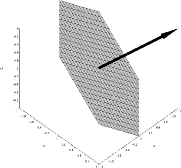
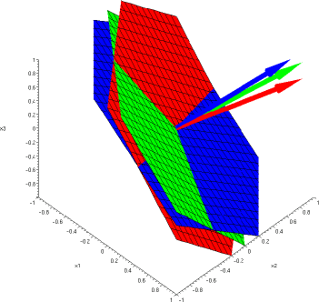
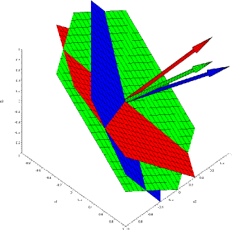
b c
The strongest condition found for the acceleration vector (RH.6) can be rewritten as
| (6.1) |
with the components of taken with respect to the normalised eigenvector basis of . This obviously means, that the vector has to lie strictly inside an ellipsoid whose semi-major axes are determined by the eigenvalues .
6.2. Trivial foliation of Minkowski space
As an example consider Minkowski space with standard coordinates . Its flat foliation by -surfaces with vanishing curvature quantities and does not fulfil the stability conditions:
Vanishing extrinsic curvature results in which violates (RH.5). However, this violation is only marginal: The situation lies exactly on the border of the condition.
Furthermore, the right hand side of (RH.6) is undefined. The formal singularity can be resolved by taking an appropriate limiting procedure (the numerator is of third order in , the denominator is only of first order), but this will still only result in the condition which cannot be satisfied. But also here, the condition (RH.6) is only marginally violated.
So it is to be expected, that the eigenvalues of the propagation tensor lie on the imaginary axis. The propagation equation with vanishing curvature quantities reads (5.1)
| (6.2) |
which is completely analogous to the Ampère-Faraday law of vacuum electrodynamics. The propagation tensor in frequency representation therefore is with its eigenvalues . As expected, their real parts vanish. Therefore flat Minkowski foliations are not stable in the strict sense used above, but instead are marginally stable. However, this might be unstable enough to spoil numerical simulations, since constraint violations will evolve undamped and so can pile up, even though the growth rate will not be significant.
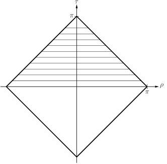
6.3. Hyperboloidal foliation of Minkowski space
Now consider the foliation of Minkowski space given by surfaces of the parametrisation
| (6.3) |
in spherical coordinates with compactified time coordinate and compactified radial coordinate (see fig. 2). The leaves in standard coordinates are shown in fig. 3.
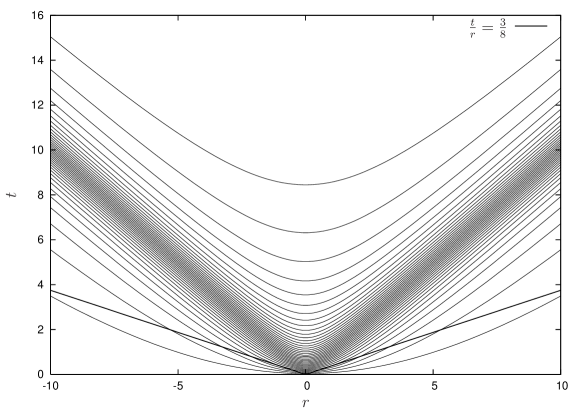
This gives for the extrinsic curvature:
| (6.4) | ||||
| (6.5) |
That means the condition (RH.5) is satisfied only for , i.e. . In this case, the acceleration vector reads
| (6.6) |
with the radial unit vector tangent to the leaf. Condition (RH.6) is just
| (6.7) |
which means that the condition holds for points which are above the straight line plotted in fig. 3.
7. Conclusion
We have shown in this work that the stability of the constraint propagation is heavily influenced by the choice of the time slicing, i.e., by the choice of the time coordinate. We derive our results by an application of the Routh-Hurwitz criterion to the propagation equation obtained by freezing the coefficients in the system of PDEs that describes the propagation of the constraints. The system we have treated is known as the Weyl system because it describes the evolution of the gravitational degrees of freedom given by the Weyl tensor. We obtain conditions for the extrinsic curvature and the acceleration vector of the foliation which have to be satisfied for the local constraint propagation to be stable.
This work can only be considered as a first step towards understanding the various contributions to the behaviour of the constraints in numerical simulations. For instance, we have ignored the effect of the Ricci rotation coefficients to the propagation tensor by focussing exclusively on the time foliation.
Furthermore, it is well known that one can add to the evolution equations terms which are homogeneous in the constraint quantities. This will generate a subsidiary system whose principal part is different from the original one and which will have different stability properties. These possibilities have also been completely ignored by us. However, general considerations (see [2]) show that such modifications cannot be successful as long as they keep the time reversal symmetry of the Einstein equations. Basically, the argument goes by considering with each initial data set the time reversed initial data set. If the perturbations of the constraints are damped in one case then by time reversal, they will grow in the other case. Thus, the constraint surface cannot be attrative.
We have also treated the Weyl system in isolation, i.e. decoupled from the rest of the system that describes the time evolution of vacuum space-times. In this larger system, there is feedback into the Weyl constraints by the constraints coming from the other subsystems and vice versa. Again, a more detailed analysis should be made in order to understand these effects.
Even though we have applied our analysis only to the case of the Weyl system it is clear that a similar analysis can also be applied to the standard ADM and the BSSN formulation. Then one could compare the analytical findings with the study by Shinkai and Yoneda. It would be interesting to see whether the much improved performance of the BSSN system compared to the ADM system can be understood from the point of view of this stability analysis. To end, we quickly recapitulate the procedure we have followed for our analysis, and which is to be applied to answer the questions given last:
-
(1)
Starting from the covariant field equations, hyperbolic reduction produces a set of constraint equations and evolution equations. The distribution of the properties of the covariant equation into the constraint and evolution equations is decided by the choice of gauge which appears as coefficients in the split equations.
-
(2)
For the constraint quantities whose vanishing indicates fulfillment of the constraint equations, propagation equations can be derived using the evolution equations. These are considered as equations for the constraint variables propagating on the fixed background provided by some solution of the full system of evolution and constraint equations.
-
(3)
The propagation equations generally couple all of the system’s constraint quantities. As a first step, feedback of one subsystem into itself can be studied by assuming the other constraint quantities to vanish which decouples the subsystem.
-
(4)
Freezing of coefficients approximates the decoupled system locally by partial differential equations with constant coefficients defined on the local tangential space.
-
(5)
These frozen propagation equations are apt to Fourier analysis yielding propagation equations in frequency representation which are just ordinary differential equations with constant coefficients.
-
(6)
The location of the complex eigenvalues of the matrix of coefficients (propagation tensor) governs the stability behaviour of constraint propagation in this localised picture. Necessary for asymptotic stability is that the real parts of the eigenvalues are negative.
-
(7)
The Routh-Hurwitz criterion is the proper tool to analyse the spectrum with respect to stability. It allows to distill algebraic conditions for the gauge parameters under which stable constraint propagation is possible.
These conditions represent necessary and sufficient conditions for locally asymptotic stability of constraint propagation within the subsystem under analysis. For the stability of the whole system, they are in general necessary conditions.
Acknowledgment
We are grateful to Prof. H. P. Hadeler for pointing out the Routh-Hurwitz criterion to us. This work has been supported by the SFB-TR7 project on ‘Gravitational wave astronomy’ of the DFG. JF is grateful to the Erwin-Schrödinger Institut in Vienna for hospitality while this paper was written. TV is grateful to the SFB 382 ‘Methods and algorithms for the simulation of physical processes on super computers’ of the DFG for supporting this research and to the Max-Planck-Institut für Gravitationsphysik (Albert-Einstein-Institut), Golm/Potsdam for the opportunity to finish his contribution to this paper.
Appendix A Simplifying assumptions
In our treatment of the propagation system it has been necessary to make some simplifying assumptions in order to bring the equations into a manageable form. Here, we want to discuss these assumptions in more detail. Let us start with the covariant form of the propagation system (5.1)
| (A.1) |
This equation is given on the space-time manifold which, we imagine, has been foliated into space-like leaves given by for some global time coordinate . The time-like vector field is chosen to be the time-like unit-vector field to the foliation. In addition, we suppose that three further space-like unit-vector fields () have been chosen in order to form a complete tetrad field with . The space-like members of the tetrad are necessarily tangent to the leaves of the foliation. Let be the dual basis. Then we can write every tensor field with respect to this basis. Thus we have e.g.,
| (A.2) |
Inserting these expansions into the equations and taking components yields for
| (A.3) |
Here, denotes the directional derivative along the tetrad vector while is the directional derivative along . Introducing the familiar (3+1)-split we may write
| (A.4) |
with the lapse function and the shift vector .
The functions and are Ricci rotation coefficients with respect to the tetrad defined by
They characterise the behaviour of the spatial tetrad vectors. Geometrically, the functions determine how the spatial triad is transported from one leaf of the foliation to the next. In the formulations we are interested in, they are considered as gauge source functions, i.e., they can be prescribed freely as functions on . Here, we will assume that they in fact vanish. This amounts to moving the spatial vectors by Fermi-Walker transport along the integral curves of , the world lines of the Eulerian observers attached to the foliation (i.e., those observers for which the current leaf is the manifold of simultaneity).
Now we fix some event which will be the point on which we localise the equation. Let be the value of the time coordinate at and let be the leaf through . Let us introduce normal coordinates inside centred at with respect to the metric and choose the spatial triad at that point to agree with the coordinate vectors. Then only at the point we have . After localisation we have (A.3) with all the coefficients being frozen at their value at . This results in
| (A.5) |
Admittedly, this procedure of removing the functions is somewhat brutal and not quite consistent. However, it is the best that we can do if we want to study the isolated influence of the time foliation on the stability properties.
Appendix B The generalised Routh-Hurwitz criterion
The appropriate tool to answer questions of stability of ODEs is the Routh-Hurwitz criterion, also known as Bilharz criterion, which originates from stability theory. Presentations of the criterion can be found in Gantmacher [17] and Parks and Hahn [22]. Our representation follows the lines of [17]:
Theorem 1 (Routh-Hurwitz).
Let be a complex polynomial of degree with
with , real and without loss of generality (otherwise assign , which does not change its roots). Now define the -dimensional Hurwitz determinant
where and for . Further let both of the following real polynomials
be coprime, which is equivalent to . Then the number of roots of the polynomial , which are located in the right complex half-plane , is given by
| (B.1) |
with denoting the number of changes of sign in the sequence . In case some of the determinants in (B.1) vanish, then for every section of vanishing determinants of length
one has to set:
| (B.2) |
The proof is rather extensive and can be found in the mentioned literature, the basic idea however will be outlined in the following section. From the theorem follows, that equivalent to asymptotic stability is, that all Hurwitz determinants are strictly positive.
B.1. Mathematical background
The basic idea behind the remarkable Routh-Hurwitz criterion is the argument principle: Every polynomial of degree has exactly complex roots and can therefore be written as a product of its elementary divisors:
| (B.3) |
Then the argument of constitutes additively from the contributions of the several elementary divisors:
| (B.4) |
Now choose a closed, non-self-intersecting path in the complex plane and track the change of while travelling once around in positive orientation (s. fig. 4).
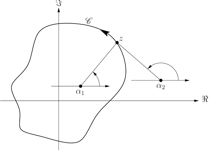
As the change of argument sums up from the contributions of each root, one can look at each root individually:
If the considered root lies outside of the domain enclosed by (e.g. in fig. 4), then the argument of first grows a little, then decreases and finally increases so that the net difference exactly vanishes. Roots out of therefore contribute nothing to the change of argument.
On the contrary, if the root under consideration lies inside (as of fig. 4 does), then the argument of grows continually, picking up an increase of for one revolution.
So the growth of argument counts the number of roots inside , counting multiple roots according to their multiplicity:
| (B.5) |
This connection between change of argument and the location of roots can now be employed to count the roots in a complex half-plane. Let and be the number of roots in the left and right half-plane, and , i.e. no roots lie on the imaginary axis. Now one can construct a path out of two segments (s. fig. 5), which encloses the left complex half-plane for .
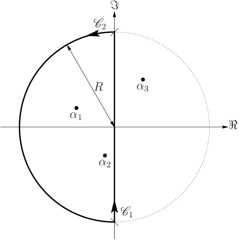
Calculating the change of argument for the individual segments, the half-circle for always counts all roots, regardless of their location:
| (B.6) | ||||
The complete path however counts only the roots in the left complex half-plane according to the argument principle:
| (B.7) |
Thus the contribution of along the imaginary axis is given as the difference of these two amounts:
| (B.8) |
This can be written as
| (B.9) |
Representing the polynomial by
| (B.10) |
with real polynomials and , and using
| (B.11) |
now allows to state the Leonhard-Michailov criterion:
All roots are located in the left complex half-plane (), if and only if
| (B.12) |
increases exactly by when travelling along the real axis from to .
That means, one has to track the change of angle of the vector
| (B.13) |
when walking from to , and count how often the vector circles around the origin. This is a rather cumbersome method. Fortunately, it is possible to find an algebraic version of this criterion. The following shall outline the necessary procedure. For a proof, we refer to literature, e.g. [22, section 1.2, p. 10ff].
As a first step, the growth of by multiples of is directly related to the number of jumps between and of . For every increase by , the fraction jumps exactly once from to .
A magnitude which counts such jumps is the Cauchy index which amounts to the number of jumps of the function from to minus the number of jumps from to , when tracing from to .
Considering rational functions , the Cauchy index can be calculated from the Sturm sequence if and are coprime and the degree of is greater than that of . The Sturm sequence is generated by the Euclidean algorithm: For two elements and of a Sturm sequence, the next element is the negative residual of the polynomial division , i.e.
| (B.14) |
where the quotient polynomials are of no further interest. As the degree is decreasing from element to element, the Sturm sequence terminates with a constant polynomial which is non-vanishing if and only if and are coprime. In this case furthermore the Sturm theorem for the Cauchy index of the rational function holds:
| (B.15) |
with denoting the number of changes of sign in the sequence . Thus one evaluates the elements of the Sturm sequence at the position and then counts the number of changes of sign.
For the Leonhard-Michailov criterion one is interested in the Cauchy index , therefore the Sturm sequence must be evaluated at and . For these limiting values only the highest order coefficients in the elements of the Sturm sequence play a role. They can be expressed in terms of special determinants, which are composed out of the coefficients of and .
Finally this leads to the Routh-Hurwitz criterion given above, which therefore represents an algebraic version of the Leonhard-Michailov criterion.
References
- [1] Robert Bartnik, Phase space for the Einstein equations, gr-qc/0402070.
- [2] Othmar Brodbeck, Simonetta Frittelli, Peter Hübner, and Oscar A. Reula, Einstein’s equations with asymptotically stable constraint propagation, J. Math. Phys. 40 (1999), 909–923.
- [3] Gioel Calabrese, Luis Lehner, and Manuel Tiglio, Constraint preserving boundary conditions in numerical relativity, Phys. Rev. D 65 (2002), 104031.
- [4] Gioel Calabrese, Jorge Pullin, Oscar Reula, Olivier Sarbach, and Manuel Tiglio, Well posed constraint-preserving boundary conditions for the linearized Einstein equations, Comm. Math. Phys. 240 (2003), 377–395, gr-qc/0209017.
- [5] Helmut Fischer and Helmut Kaul, Mathematik für Physiker, vol. 2, B. G. Teubner, Stuttgart, 1998 (german).
- [6] Arthur Fisher and Jerrold E. Marsden, The initial value problem and the dynamical formulation of general relativity, General Relativity: An Einstein Centenary Survey (Stephen W. Hawking and Werner Israel, eds.), Cambridge University Press, Cambridge, 1979, pp. 138–212.
- [7] Jörg Frauendiener, Conformal infinity, Living Reviews in Relativity 7 (2004), no. 1, Update, http://www.livingreviews.org/lrr-2004-1/.
- [8] Jörg Frauendiener, On the Velo-Zwanziger phenomenon, J. Phys. A 36 (2003), 8433–8442.
- [9] Helmut Friedrich, Cauchy problems for the conformal vacuum field equations in general relativity, Comm. Math. Phys. 91 (1983), 445–472.
- [10] by same author, Einstein equations and conformal structure: Existence of anti-de Sitter-type space-times, J. Geom. Phys. 17 (1995), 125–184.
- [11] by same author, Hyperbolic reductions for Einstein’s field equations, Class. Quantum Grav. 13 (1996), 1451–1469.
- [12] Helmut Friedrich and Gabriel Nagy, The initial boundary value problem for Einstein’s vacuum field equations, Comm. Math. Phys. 201 (1998), 619–655.
- [13] Simonetta Frittelli, Note on the propagation of the constraints in standard general relativity, Phys. Rev. D 55 (1997), 5992–5996.
- [14] Simonetta Frittelli and Roberto Gómez, Boundary conditions for hyperbolic formulations of the Einstein equations, Class. Quantum Grav. 20 (2003), 2379–2392, gr-qc/0302032.
- [15] by same author, Einstein boundary conditions for the 3+1 Einstein equations, Phys. Rev. D 68 (2003), 044014, gr-qc/0302071.
- [16] by same author, Einstein boundary conditions in relation to constraint propagation for the initial-boundary value problem of the Einstein equations, Phys. Rev. D 69 (2004), 124020, gr-qc/0310064.
- [17] F.R. Gantmacher, Matrizenrechnung II, Hochschulbücher für Mathematik, vol. 37, VEB Deutscher Verlag der Wissenschaften, Berlin, 1959 (german), Translation from Russian to German: Klaus Stengert.
- [18] Michael Holst, Lee Lindblom, Robert Owen, Harald P. Pfeiffer, Mark A. Scheel, and Lawrence E. Kidder, Optimal constraint projection for hyperbolic evolution systems, gr-qc/0407011.
- [19] Sascha Husa, Numerical relativity with the conformal field equations, Lect. Notes Phys. 617 (2003), 159–192, gr-qc/0204057.
- [20] Heinz Otto Kreiss and Jens Lorenz, Initial-boundary value problems and the Navier-Stokes equations, SIAM, Philadelphia, 2004.
- [21] Lee Lindblom, Mark A. Scheel, Lawrence E. Kidder, Harald P. Pfeiffer, Deirdre Shoemaker, and Saul A. Teukolsky, Controlling the growth of constraints in hyberbolic evolution, Phys. Rev. D 69 (2004), 124025, gr-qc/0402027.
- [22] Patrick Christopher Parks and Volker Hahn, Stabilitätstheorie, Springer, Berlin; Heidelberg; New York, 1981 (german), ISBN 3-540-11001-1.
- [23] Roger Penrose, Zero rest-mass fields including gravitation: asymptotic behaviour, Proc. Roy. Soc. London A 284 (1965), 159–203.
- [24] Hisa-aki Shinkai and Gen Yoneda, Re-formulating the Einstein equations for stable numerical simulations: Formulation problem in numerical relativity, gr-qc/0209111.
- [25] by same author, Constraint propagation in the family of ADM systems, Phys. Rev. D 63 (2001), 124019, gr-qc/0103032.
- [26] by same author, Adjusted ADM systems and their expected stability properties: constraint propagation analysis in Schwarzschil spacetime, Class. Quantum Grav. 19 (2002), 1027–1050, gr-qc/0110008.
- [27] by same author, Advantages of modified ADM formulation: constraint propagation analysis of Baumgarte-Shapiro-Shibata-Nakamura system, Phys. Rev. D 66 (2002), 124003, gr-qc/0204002.
- [28] John Stewart, The Cauchy problem and the initial boundary value problem in numerical relativity, Class. Quantum Grav. 15 (1998), 2865–2889.
- [29] W. Gilbert Strang, Necessary and insufficient conditions for well-posed Cauchy problems, J. Diff. Eqn. 2 (1966), 107–114.
- [30] Béla Szilágyi, Roberto Gómez, Nigel Bishop, and Jeffrey Winicour, Cauchy boundaries in linearized gravitational theory, Phys. Rev. D 62 (2000), 104006, gr-qc/9912030.
- [31] Béla Szilágyi, Bernd Schmidt, and Jeffrey Winicour, Boundary conditions in linearized harmonic gravity, Phys. Rev. D 65 (2002), 064015, gr-qc/0106026.
- [32] Béla Szilágyi and Jeffrey Winicour, Well-posed initial-boundary evolution in general relativity, Phys. Rev. D 68 (2003), 041501, gr-qc/0205044.
- [33] Manuel Tiglio, Dynamical control of the constraints growth in free evolutions of Einstein’s equations, gr-qc/0304062.
- [34] Tilman Vogel, Stabilitätsbedingungen für die Propagation der Zwangsbedingungen in der Allgemeinen Relativitätstheorie, Diplomarbeit, Eberhard-Karls-Universität Tübingen, April 2004, http://www.tat.physik.uni-tuebingen.de/~scri/Thesis/200404-vogel.pdf.
- [35] Gen Yoneda and Hisa-aki Shinkai, Diagonalizability of constraint propagation matrices, Class. Quantum Grav. 20 (2003), L31–L36, gr-qc/0209106.