Horizon Pretracking

Abstract

We introduce horizon pretracking as a method for analysing numerically generated spacetimes of merging black holes. Pretracking consists of following certain modified constant expansion surfaces during a simulation before a common apparent horizon has formed. The tracked surfaces exist at all times, and are defined so as to include the common apparent horizon if it exists. The method provides a way for finding this common apparent horizon in an efficient and reliable manner at the earliest possible time. We can distinguish inner and outer horizons by examining the distortion of the surface. Properties of the pretracking surface such as its expansion, location, shape, area, and angular momentum can also be used to predict when a common apparent horizon will appear, and its characteristics. The latter could also be used to feed back into the simulation by adapting e.g. boundary or gauge conditions even before the common apparent horizon has formed.

I Motivation

In a spacetime that contains coalescing binary black holes, and given suitable gauge conditions, a common apparent horizon forms some time after the event horizons have merged. Similarly, in a spacetime containing a collapsing star, an apparent horizon forms some time after the event horizon has formed. In numerical calculations it is important to locate apparent horizons. On one hand, one can extract interesting physical information from an apparent horizon, such as the object’s mass and spin, for instance via the dynamical horizon formalism Ashtekar and Krishnan (2004); Dreyer et al. (2002). On the other hand, certain numerical methods such as excision boundaries Cook et al. (1998); Alcubierre et al. (2001) use the apparent horizon to identify the region within the black hole. Knowing the common horizon location also makes it possible to adjust the dynamics of the spacetime via so-called “horizon-locking” gauges Anninos et al. (1995a); Balakrishna et al. (1996), as well as gauges which attempt to control the location of the black hole Alcubierre et al. . At late times, the shape and oscillations of the apparent horizon is an effective indicator of the angular momentum of the final black hole, and has been related to its quasi-normal mode ringing Anninos et al. (1995b).

From a practical standpoint, it is the apparent horizons which are more interesting than the event horizon at a given instant of time, since the latter is a globally defined quantity whose location can only be determined once the entire future development of the spacetime is known. The apparent horizon, on the other hand, is defined by the outermost marginally trapped surface and can be found locally in time. Further, it is always contained within the event horizon Hawking and Ellis (1973) when the strong energy condition holds, making it a “safe” estimator of the black hole location for use by excision boundaries Thornburg (1987); Seidel and Suen (1992).

A typical simulation scenario involves a pair of binary black holes, identified by disconnected horizons in the initial data surface, evolving until they come close enough that a common horizon forms around them. The common apparent horizon appears instantaneously as a surface enveloping the two individual horizons. This is different from the situation for event horizons, where the disconnected lobes “grow together” to form a single connected surface Hawking and Ellis (1973); Anninos et al. (1995b). For a given dynamical evolution, it is not known a priori when and where a common apparent horizon first appears, as this depends on both the initial data as well as the particular slicing of the spacetime.

Fast apparent horizon finders, which essentially solve a nonlinear elliptic equation, require a good initial guess for both the location and shape of the surface Thornburg (1996). For horizons which are present in the spacetime from the initial time, it is usually sufficient to use the previously detected surface as an estimate for the horizon location at some small time interval later. The initial data construction itself often provides a good first guess for individual horizons. The common horizon, however, appears instantaneously at some late time and without a previous good guess for its location. In practice, an estimate of the surface location and shape can be put in by hand. The quality of this guess will determine the rate of convergence of the finder and, more seriously, also determines whether a horizon is found at all. Gauge effects in the strong field region can induce distortions that have a large influence on the shape of the common horizon, making them difficult to predict, particularly after a long evolution using dynamical coordinate conditions. As such, it can be a matter of some expensive trial and error to find the common apparent horizon at the earliest possible time. Further, if a common apparent horizon is not found, it is not clear whether this is because there is none, or whether there exists one which has only been missed due to unsuitable initial guesses — for a fast apparent horizon finder, a good initial guess is crucial.

In this paper, we present a reliable method for determining the first common horizon to appear in a dynamical spacetime evolution. The method provides a close to optimal initial guess for the horizon surface and reliable predictions of its physical properties. Roughly speaking, horizon pretracking Schnetter (2003) involves searching the spacetime for the surface of minimal constant expansion which envelops the source. For a spacetime without a common horizon, this surface will have positive expansion. Assuming that a common horizon does form after some time, the expansion of the pretracking surface will gradually decrease to zero with time, at which point the common horizon has formed, by definition.

The rationale for this method is that it is much more reliable and efficient to “track” a surface than to find an entirely new surface, the difference being that a good initial guess is provided by the previous value of the tracked surface. In the past, a method such as pretracking might have been too computationally expensive to be implemented as a practical solution. However, careful consideration of the problem of finding constant expansion surfaces has resulted in algorithms which typically solve the system in a matter of seconds Thornburg (1996); Schnetter (2003); Thornburg (2004). Thus the required search for the minimal expansion surface becomes feasible.

Pretracking has some similarities to minimisation Anninos et al. (1998); Metzger (2004) or curvature Shoemaker et al. (2000) flow methods for apparent horizon finding. These methods solve a minimisation problem or a parabolic equation to find horizons, starting from a large sphere, and can give a reliable answer as to whether a common horizon exists. Their disadvantage is that these methods are extremely slow and cannot be applied at every time step. Pretracking is faster since it “tracks” instead of minimising or “flowing” at each time. Additionally, the pretracking surfaces can provide valuable information about the current state of the simulation.

In Section II we briefly discuss surfaces of constant expansion. Section III defines the notion of a pretracking surface, and outlines a number of algorithmic details involving the parametrisation of the surface, and the binary search method for the minimal constant expansion surfaces. Finally in Section IV we present applications of the technique to binary black hole mergers.

II Apparent Horizons and Constant Expansion Surfaces

An apparent horizon (AH) is the outermost marginally outer-trapped surface in a spacelike hypersurface $\Sigma$. The AH satisfies the conditions $\Theta_{(\ell)}=0$ and $\Theta_{(n)}<0$, where $\Theta_{(\ell)}$ and $\Theta_{(n)}$ are the expansions of the outgoing and ingoing null normals of the surface. These can be calculated from the ADM variables via

$$\Theta_{(\ell)} = +\nabla_{i}s^{i}+K_{ij}(s^{i}s^{j}-\gamma^{ij})\quad\textrm{and}$$ (1)

$$\Theta_{(n)} = -\nabla_{i}s^{i}+K_{ij}(s^{i}s^{j}-\gamma^{ij})\textrm{.}$$ (2)

Here $\gamma_{ij}$ and $K_{ij}$ are the three-metric and extrinsic curvature of the spacelike hypersurface, and $s_{i}$ is the spacelike normal to the surface within the spacelike hypersurface.

We describe the surface explicitly through a function $h(\theta,\phi)$ which specifies the radius of the surface as function of the angular coordinates $\theta$ and $\phi$ about some origin. The spacelike normal is then given by $s_{i}=\nabla_{i}F/|\nabla F|$, where $F(r,\theta,\phi)=r-h(\theta,\phi)$ with the coordinate radius $r$, hence $F(r,\theta,\phi)=0$ indicates the surface location. This explicit representation is convenient but not necessary for surfaces with $S^{2}$ topology, and is not restrictive in practice Thornburg (2004).

The notion of pretracking requires specifying a general family of surfaces for spacetimes which may not have an apparent horizon, but which contain the AH as a surface if one exists. For instance, a generalisation to the concept of apparent horizons are the constant expansion (CE) surfaces, which are defined by the condition

$$\Theta_{(\ell)} = C,$$ (3)

with $C$ a constant over the surface Schnetter (2003). The apparent horizon is a CE surface with $C=0$. For $K_{ij}=0$, the CE surfaces are identical to constant mean curvature (CMC) surfaces, which are defined by $\nabla_{i}s^{i}=C$. In an asymptotically flat spacetime with zero extrinsic curvature, the CMC surfaces foliate the hypersurface in a neighbourhood of infinity Huisken and Yau (1996). Thus a parametrised family of CMC surfaces can be specified at large radii, though they may not exist in the strong field interior of a spacelike slice. In numerical experiments with isolated sources, we have found that CE surfaces form a similarly useful foliation at large distances even for $K_{ij}\neq 0$ Schnetter (2003).

A simple algorithm for pretracking can be described as follows: Define a parametrised family of CE surfaces $h_{p}(\theta,\phi)$ which envelop the source, via

$$h_{p}(\theta,\phi) : \Theta_{(\ell)}[h_{p}]=C_{p},$$ (4)

where $p$ labels each member. Here we introduce the notation $[h]$ to indicate that a quantity is a functional of the surface function $h(\theta,\phi)$. The surface with the smallest positive expansion $C_{p}$ forms the “best guess” for the location of the AH. For time evolutions of vacuum spacetimes, this surface is expected to change continuously, and can be followed until the expansion of the surface reaches zero, at which point it represents the earliest common AH.

A difficulty arises from the above definition of the pretracking surface $h_{p}$ which introduces some practical complications. While the expansion is zero at the location of the AH, it also decreases to zero asymptotically towards spacelike infinity, while being positive in between. This is illustrated in Fig. 1 for flat space in Minkowski coordinates and for a black hole in Brill-Lindquist and Kerr-Schild coordinates. For horizon finding we are more interested in the surfaces most closely enveloping the source. Thus, the initial guess must be chosen inside the maximum of $\Theta$ if the method is to avoid converging to one of the asymptotic surfaces. To remove this ambiguity, a more suitable function would increase monotonically outside the common AH. In practice, one therefore has to use a modified minimisation criterion, as described below.

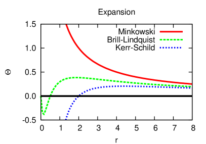
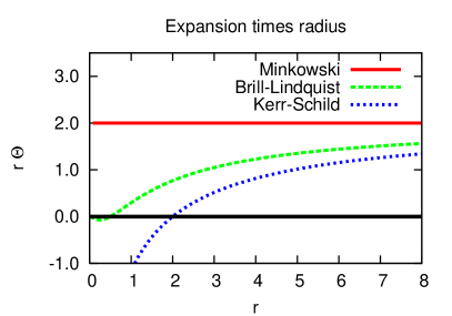
Figure 1: Expansion $\Theta$ and the quantity $r\Theta$ vs. coordinate radius $r$ for flat space in Minkowski coordinates and for a black hole in Brill-Lindquist and Kerr-Schild coordinates. Both $\Theta=0$ and $r\Theta=0$ define the location of the apparent horizon, which is at different radii in different coordinate systems. While $\Theta$ reaches a maximum at a finite radius, $r\Theta$ increases monotonically in spherical symmetry.

III Horizon Pretracking

III.1 Method

The pretracking method attempts to find a surface corresponding to a “generalised apparent horizon”. That is, we would like to find a horizon-like surface which envelops a compact source, even at times when an actual common horizon does not exist, but which reduces to the apparent horizon when it is present. The generalised surface is found among a specified parametrised family, $\{h_{p}\}$. The pretracking method corresponds to finding the “smallest” member of the family, i.e., the value of the parameter $p$ such that the surface $h_{p}(\theta,\phi)$ satisfies

$$H[h_{p}] = \mathrm{const},$$ (5)

$$G[h_{p}] \stackrel{{\scriptstyle!}}{{=}} \mathrm{min},$$ (6)

where the shape function $H[h]$ is a generalisation of the expansion $\Theta_{(\ell)}$, and the goal function $G[h]$ specifies what we mean by “smallest”. Note that $H$ maps to a function, while $G$ maps to a scalar.

The parametrised family $\{h_{p}\}$ should be defined in such a way as to contain the common AH if it exists in the given slice. The shape function, $H$, specifies the surfaces that we want to find. We allow here for a more generic set of surfaces than only CE surfaces. The goal function, $G$, defines a suitable notion of “closeness” among the surfaces $H_{p}$ to an actual apparent horizon. As such, it is useful to define it in such a way that it evaluates to zero for a surface which is a common AH, negative within the AH, and monotonically increasing outside the AH.

We generalise the concept of CE surfaces for a number of pragmatic reasons. For instance, very distorted surfaces are difficult or impossible to represent accurately in terms of a function $h(\theta,\phi)$, so we have found more rounded surfaces work consistently better. We have experimented with the following shape functions:

$$H_{1}[h] := \Theta_{(\ell)}[h],$$ (7)

$$H_{r}[h] := \Theta_{(\ell)}[h]\cdot h,$$ (8)

$$H_{r^{2}}[h] := \Theta_{(\ell)}[h]\cdot h^{2}.$$ (9)

As above, $h(\theta,\phi)$ is the shape of the surface, i.e., the surface’s coordinate radius at the coordinate angles $\theta,\phi$. The first definition, $H_{1}$, is simply the surface’s expansion, so that the condition $H_{1}[h]=\mathrm{const}$ specifies CE surfaces. We find empirically that the shape functions $H_{r}$ and $H_{r^{2}}$ lead to surfaces with a less distorted coordinate shape. (This can be seen e.g. in the lower left hand graph of Figure 6.) The shapes $H_{r}$ and $H_{r^{2}}$ are in general not CE surfaces, but they tend to CE surfaces for large radii and close to the apparent horizon.

Note that $H_{r}$ and $H_{r^{2}}$ are not defined in a covariant manner, because their definition depends on the coordinate shape. While we would prefer covariant shapes, we find that the listed non-covariant shapes work much better in practice and are computationally more efficient. Empirically, especially the shape function $H_{r}$ leads to a reliable pretracking method. All of the above surface shapes are apparent horizons if and only if the shape function is zero everywhere.

The goal function $G[h]$ must have a minimum for the surface $h_{p}$ that we want to call “closest” to being an AH. That is, the goal function has a minimum which is located at the AH when one exists. We considered the following goal functions:

$$G_{H}[h] := \overline{H[h]},$$ (10)

$$G_{Hr}[h] := \overline{H[h]}\cdot\overline{h},$$ (11)

$$G_{r}[h] := \overline{h},$$ (12)

where the over-bar $\overline{\cdot}$ denotes the average over the surface. We take this average as an average over all grid points. One could alternatively define a covariant average that takes the two-metric into account, but we did not consider the advantage of this to be worth the additional complexity in the equations for the Jacobians (cf. Section III.2 and Appendix A). For a solution $h$, we require not only a specific value of $G$, but also that $H[h]$ be constant over the surface, so that e.g. $G_{Hr}=0$ implies $H=0$ everywhere.

The combination of the shape function $H_{1}$ and the goal function $G_{H}$ leads to the simple algorithm mentioned in the previous section. As already discussed, the difficulty with this choice is that even in spherical symmetry, the goal function is not monotonic, but rather reaches a maximum at a finite radius. Thus, this method is not expected to converge unless an appropriate initial surface, within the maximum, is chosen. One way to resolve this ambiguity is to redefine the shape function, for instance via (8) or (9). For either of these surface functions, the goal function $G_{H}$ increases monotonically (at least in spherical symmetry) and is zero on the AH. The lower graph of Fig. 1 shows the goal function $G_{H}$ for the shape function $H_{r}$, i.e., the quantity $r\Theta$.

The combination of the shape function $H_{1}$ and the goal function $G_{Hr}$ also ensures a monotonically increasing goal function in spherical symmetry, with the additional advantage that all pretracking surfaces are CE surfaces, and thus covariantly defined. Unfortunately we find empirically that this combination does not work as well in practice as the combination of $H_{r}$ and $G_{H}$ (see Section IV).

The goal function $G_{r}$ measures the average coordinate radius of a given surface, so that the method selects the surface with smallest average coordinate radius satisfying $H[h]=0$. Note however, that the AH does not usually form at the innermost surface defined by $H$ (as shown in in Section IV). Thus this goal function cannot reliably be used for pretracking, although it can still be very useful to study the behaviour of the innermost CE surface.

Finally, we note that the goal functions $G_{Hr}$ and $G_{r}$ are not covariantly defined, as they depend on the coordinate radius of the surface. This is not an issue, as the value of the goal function itself has no relevance other than the value $G[h]=0$, which by definition is the covariantly defined AH.

III.2 Surface Finding

Finding a surface $h(\theta,\phi)$ that satisfies one of the above conditions $H[h]=\mathrm{const}$ under a constraint $G[h]=p$ for a given value $p$ is comparable to finding an apparent horizon. Efficient implementations of apparent horizon finders have been developed in recent years Schnetter (2003); Thornburg (2004), and it is a straightforward extension to allow them to look for alternate similarly defined surfaces, such as those defined by the $H_{*}$ listed above. Current efficient AH finders interpret the surface defining equation as a nonlinear elliptic equation; they use a Newton-Raphson iteration method to linearise and then a Krylov subspace method to solve it.

The overall elliptic equation that defines the pretracking surface is

$$H[h](\theta,\phi)-\overline{H[h]}+G[h]-p = 0,$$ (13)

which is fulfilled if and only if $H[h]$ is constant over the surface and if $G[h]=p$. This is because the first term $H[h]$ is the only term that varies over the surface, and therefore it has to be constant for the equation to be fulfilled. In this case, the expression $H[h]-\overline{H[h]}$ vanishes, which then implies $G[h]=p$. Discretised, this equation becomes

$$H_{i}(h_{j})-\frac{1}{N}\sum_{k}H_{k}(h_{j})+G(h_{j})-p = 0,$$ (14)

where $i,j,k$ label grid points, and $N$ is the total number of grid points on the horizon surface. The Jacobian of this equation is

$$J_{ij}-\frac{1}{N}\sum_{k}J_{kj}+\partial_{j}G,$$ (15)

where $J_{ij}=\partial H_{i}/\partial h_{j}$ is the Jacobian of the surface shape function $H_{i}$, and $\partial_{j}G=\partial G/\partial h_{j}$. For example, when $H$ is the shape function $H_{1}$, the Jacobian $J_{ij}$ is the Jacobian of the original apparent horizon equation.

There is one crucial problem that appears when one attempts to solve equation (14). The Newton-Raphson method requires the Jacobian of the equation to be sparsely populated, otherwise the method will be prohibitively expensive. Unfortunately, the Jacobian (15) is densely populated due to the term $\sum_{k}J_{kj}$, which is nonzero for all values of the indices $i$ and $j$. For $N$ grid points, this increases the storage requirements by a factor $O(N)$, and turns the $O(N^{3/2})$ runtime cost of the solver into a cost of $O(N^{3})$. This is in general not acceptable.

We arrive at a sparse matrix by extending the vector space of the solution $h_{i}$ by one element. Instead of (14), we write the equivalent system

$$H_{i}(h_{j})-C = 0,$$ (16)

$$C-\frac{1}{N}\sum_{k}H_{k}(h_{j})+G(h_{j})-p = 0,$$

where we have introduced one additional unknown $C$ and one additional equation that determines it. The Jacobian of this equation is

$$\left(\begin{array}[]{c|c}\displaystyle J_{ij}&\displaystyle-1\\ \hline\cr\displaystyle-\frac{1}{N}\sum_{k}J_{kj}+\partial_{j}G&\displaystyle+1\end{array}\right)\quad\textrm{.}$$ (17)

This Jacobian is now sparsely populated. In addition to the already sparsely populated $J_{ij}$, it has one additional fully populated row and column, so that it has $O(N)$ nonzero entries out of $O(N^{2})$ total. The system (16) can therefore be solved efficiently.

We list the full expressions for the Jacobians for the different shape and goal functions in Appendix A.

III.3 Pretracking Search

At each time step during an evolution, pretracking consists of determining the parameter $p$ which selects a member $h$ of the family of CE surfaces $\{h_{p}\}$ that minimises the goal function $G[h]$. A convenient initial guess for $p$ is either the value from the last pretracking time or a manually specified guess, for instance corresponding to a large sphere. Because the equation defining the surface is nonlinear, it is also necessary to specify an initial guess for the surface shape $h$ itself, again either from a previously determined surface or manual specification.

We have modified an apparent horizon finder so that we can specify the desired shape function $H$, the goal function $G$, the desired parameter value $p$, and an initial guess $h_{0}$ for the surface. The result is either a surface $h$ that satisfies $H[h]=\mathrm{const}$ and $G[h]=p$, or a flag indicating that no such surface could be found.

The pretracking surface generally exists only for a certain parameter range $p>p^{*}$, i.e., only for values of $p$ above some critical parameter $p^{*}$. During the search, we keep track of an interval $[p_{\mathrm{min}},p_{\mathrm{max}}]$ that indicates which values of $p$ are known to fail and succeed, respectively. We start with a trial value of $p$ that was the result of the last pretracking time, and depending on whether the corresponding surface can be found or not, we set either $p_{\mathrm{min}}$ or $p_{\mathrm{max}}$. We then increase or decrease $p$ in large steps until we find the other end of the interval. Finally, we use a binary search within the interval to find $p^{*}$ to a given accuracy $\Delta p$, and call the resulting surface the pretracking surface at this time.

Each step of the above algorithm, i.e., each check of a parameter value $p$, is computationally equivalent to finding an apparent horizon with the advantage of a good initial guess provided by the previous search. This takes usually less than a second per step on current hardware, independent of the resolution of the underlying spacetime. Various trade-offs can be made to improve efficiency. For instance, pretracking need not be carried out at every time step of an evolution, but rather at longer intervals. We usually determine $p^{*}$ to only a moderate accuracy at each pretracking time.

In order to find the common apparent horizon as early as possible, we follow up with a regular apparent horizon search using the pretracking surface as initial guess, which is a very good initial guess near the time when the common AH forms. This finds the common apparent horizon even when pretracking is not accurate, and also allows us to pretrack in larger time intervals. The inaccuracy in the horizon guess provided by pretracking comes mainly from the fact that failure to find a pretracking surface for a certain parameter value $p$ does not necessarily indicate that the surface does not exist. Since we usually compromise some accuracy for efficiency in the pretracking search, it may be that we did not iterate long enough or did not start with a good enough initial guess for this value of $p$.

III.4 Apparent Horizon Tracking

When a common apparent horizon first forms, we find that it bifurcates into an inner and an outer horizon. This has, for example, been described by Thornburg Thornburg (2004) (cf. his Figures 3 and 4). If the apparent horizon world tube is spacelike, then the spacelike hypersurface $\Sigma$ can intersect (“weave”) the world tube in arbitrary ways, and generically, such intersections will occur in pairs. This can be seen e.g. in (Shapiro and Teukolsky, 1985, Fig. 3), which outlines the trapped region in a spherical collapse. At early times, the trapped region’s boundary is spacelike. The outer boundary, which corresponds to the apparent horizon, approaches the event horizon at late times. The structure of individual, inner, and outer horizons is also visible in (Bishop, 1982, Fig. 1) or (Cook and Abrahams, 1992, Fig. 1).

We demonstrate this for the Brill-Lindquist data in the next section. For black hole evolutions, one usually chooses gauge conditions that have the effect of making the inner horizon quickly shrink in coordinate space, while the outer horizon initially grows and then stays roughly constant in radius.

Of course, we would like to ensure that horizon tracking follows the outer horizon, as it is the one of physical interest to observers in the exterior spacetime. However, unless special measures are taken, the horizon finder will select a branch at random. We observe that shortly after bifurcation the outer horizon is generally less distorted in coordinate shape in a binary black hole merger. Before the inner and outer horizons have clearly separated in coordinate space, the tracker can also jump between the two branches. We can make the horizon tracker select the outer horizon by smoothing its initial guess. Similarly, we can make it select the inner horizon through a more distorted initial guess. Additionally, by slightly enlarging or shrinking the initial guess, the outer or inner horizons are preferred, respectively. We implement this by modifying the initial guess, $h_{0}$, before each horizon search by the prescription

$$h_{0} \rightarrow (1-f)\cdot g\cdot h_{0}+f\cdot g\cdot\overline{h_{0}},$$ (18)

where $\overline{\cdot}$ is the average over the surface. The smoothing factor, $f$, should be positive for smoothing and negative for roughening. We find that $f=0.25$ is a good smoothing choice for the particular data we examined. The enlargement factor $g$ must be positive, and will grow (or shrink) the surface if it is larger (or smaller) than one. We find that $g=1.1$ is usually a reasonable value to ensure that an outer horizon is found. On the other hand, $f=-0.2$ and $g=0.8$ selects the inner horizon in our example of a head-on collision discussed in the next section.

IV Applications

We applied the algorithms described in the previous sections to 3D simulations of (1) an axi-symmetric head-on collision and (2) coalescing binary black holes with angular momentum. For the time evolution we used the conformal-traceless (BSSN) formalism introduced in Nakamura et al. (1987); Shibata and Nakamura (1995); Baumgarte and Shapiro (1999). The particular implementation we use, including gauges ($1+\log$ lapse and $\Gamma$-driver shift) and boundary conditions, is described in Alcubierre et al. (2003). The binary black hole initial data are calculated via the puncture method Brandt and Brügmann (1997). Spins of the surfaces were measured via the dynamical horizon formalism, as described in Dreyer et al. (2002). Our time evolution code is implemented in the Cactus framework Cactus .

Pretracking was performed using extensions to Thornburg’s AHFinderDirect horizon finder Thornburg (2004). A number of different shape and goal functions were tested. These are listed in Table 1, along with corresponding labels which will be referenced in the plots in this section.

Label	Shape	Goal	tracked
	function	function	horizon
$\Theta$	$H_{1}$	$G_{H}$	outer
$r\Theta$	$H_{r}$	$G_{H}$	outer
$r^{2}\Theta$	$H_{r^{2}}$	$G_{H}$	outer
$r$-bar $\Theta$	$H_{1}$	$G_{Hr}$	outer
smallest $r$	$H_{1}$	$G_{r}$	outer
inner $r\Theta$	$H_{r}$	$G_{H}$	inner

Table 1: Algorithms described in this paper are listed according to their use of shape functions and goal functions. The methods tested in this paper correspond to the various shape and goal functions defined in Section III.1. The names listed in the leftmost column are used to label curves in the figures in this section.

IV.1 Head-on Collision

As a first test case, we studied a simple axi-symmetric head-on collision of two black holes with time-symmetric Brill-Lindquist initial data Brill and Lindquist (1963), evolved in 3D. The black holes have a mass parameter $m=1$, and are located on the $z$-axis coordinate locations $z=\pm 1$. The total ADM mass of the system is therefore $M=2$. The resolution for the particular runs performed here is $\Delta x=1/8$, and the outer boundaries were placed at coordinate $x_{\mathrm{max}}=y_{\mathrm{max}}=4$ and $z_{\mathrm{max}}=5$. We chose a pretracking surface and apparent horizon resolution of $5^{\circ}$ and a pretracking accuracy of $\Delta p=10^{-4}$.

As the singularities are punctures, we evolved them without excision by ensuring that their locations are staggered between grid points Alcubierre et al. (2003). For the lapse, $\alpha$, we used a $1+\log$ slicing condition, starting from $\alpha=1$, and used normal coordinates, $\beta^{i}=0$ throughout the evolution. The simulation was performed with an explicit octant symmetry. The model is particularly useful as a test case, as it begins with disconnected apparent horizons, but very soon (after $t\approx 1$) forms a common horizon, requiring minimal resources in terms of computation time or memory for the given resolutions and boundary locations.

Figure 2 shows various pretracking results from this evolution. The top left graph shows the average of the expansion $\Theta$ versus time for pretracking surfaces from the various algorithms listed in Table 1. The algorithms $\Theta$, $r\Theta$, $r^{2}\Theta$, and $r$-bar $\Theta$ all find the common apparent horizon at identical times, around $t=1$. (However, the algorithm $r$-bar $\Theta$ unfortunately fails in more realistic simulations; see e.g. Figure 6.) The algorithm smallest $r$ fails to find the common horizon. It locates the CE surface with smallest average radius, a surface which has a positive average expansion even after a common apparent horizon has formed. This surface actually intersects the pretracking surfaces defined by the other algorithms, and seems “smallest” due to the averaging of the radius over the surface which includes a narrow throat.

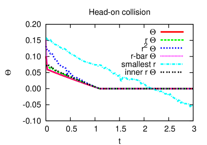
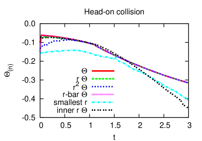
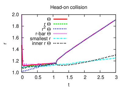
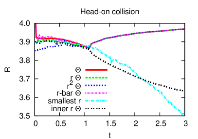
Figure 2: Averages of the expansion $\Theta$, inner expansion $\Theta_{(n)}$, coordinate radius $r$, and areal radius $R$ for a head-on collision vs. coordinate time $t$. Except for the smallest $r$ case, the common apparent horizon is found when $\Theta=0$. Shown are the results for five different pretracking algorithms. The methods labelled $\Theta$, $r\Theta$, $r^{2}\Theta$, and $r$-bar $\Theta$ track minimum surfaces of the corresponding quantity, as described in the main text. The smallest $r$ algorithm tracks the CE surface with the smallest coordinate radius, and fails to converge to the apparent horizon. Finally, inner $r\Theta$ uses the same pretracking algorithm as $r\Theta$, but locks onto inner instead of outer horizons. The roughly parabolically shaped region between the inner and outer horizons in the lower left hand graph contains trapped surfaces.

The top right plot shows the average of the expansion of the ingoing null normal $\Theta_{(n)}$ which must be negative for apparent horizons. The lower two graphs show the average coordinate radius (left) and areal radius (right) versus time of the pretracking surface. After an initial transient, all of the pretracking algorithms behave similarly, with the exception of the smallest $r$, which fails as a pretracking surface. The gradual growth in coordinate radius of the common apparent horizon is caused by the shift condition; a zero shift is unsuitable for a long-term evolution since the black hole eventually encompasses the grid. Note that the inner $r\Theta$ algorithm tracks as desired the inner apparent horizon (as described in the previous section), which has a smaller radius.

Before a common horizon is formed, the different pretracking algorithms actually determine different surfaces. Figure 3 shows the shapes of the pretracking surfaces at $t=0$, $1$, and $1.5$ in one quadrant of the $xz$-plane. Although the three successful pretracking algorithms determine rather different surfaces initially, they have converged by $t=1$, shortly before the first common apparent horizon is found. At $t=1.5$ the first three algorithms continue to track the same outer horizon surface, while the difference between the outer and inner apparent horizon (as tracked by the inner $r\Theta$ method) is clearly visible. The algorithm smallest $r$, which fails, tracks a very different surface. This surface is nevertheless interesting because it is, up to numerical errors, the smallest CE surface that exists within the given slices.

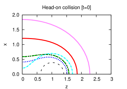
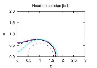
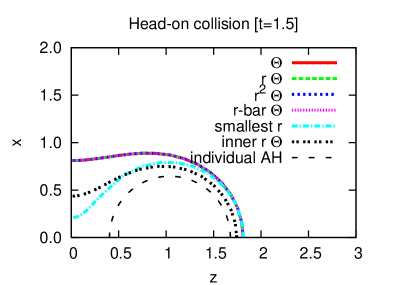
Figure 3: Shapes of the pretracking surfaces for various pretracking methods at different times. The coordinate time $t=0$ shows the initial data. The time $t=1$ is shortly before the common apparent horizon is detected. Here the different pretracking algorithms already produce very similar results. At $t=1.5$ a common apparent horizon has formed, and the inner and outer horizons have separated. The individual apparent horizons are also shown for comparison with the pretracking surfaces. The region between the inner and outer horizons in the lowermost graph contains trapped surfaces.

IV.1.1 Evolution of CE Surfaces

It is interesting to study the behaviour of various CE surfaces independent of the pretracking algorithm. Figure 4 compares how CE surfaces with constant areal radius $R$ and CE surfaces with constant expansion $\Theta$ evolve in time. Inside an inner cutoff, the CE surface equation has no solution. We are using normal coordinates, and constant areal radius surfaces grow in coordinate space. New common CE surfaces with smaller areal radii and smaller expansions begin to exist near the inner cutoff. One of these new surfaces is the common apparent horizon with expansion $\Theta=0$.

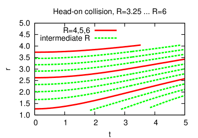
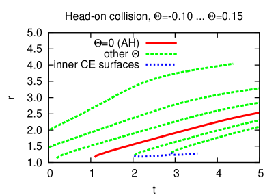
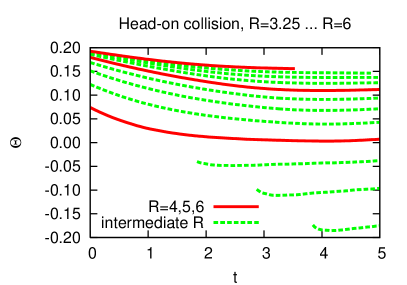
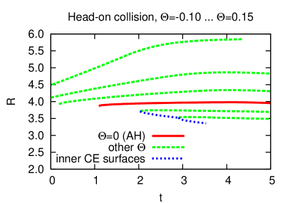
Figure 4: Left (top and bottom): Time evolution of various CE surfaces with given areal radii $R$. The graphs show CE surfaces with areal radii from $3.25$ to $6$ (from bottom to top). The upper left graph shows that these surfaces grow with time, the lower left graph shows that their expansion decreases with time. The largest CE surface is not found after $t\approx 3.5$ any more because it reached the outer boundary. The three smallest CE surfaces only begin to exist after some time.
Right (top and bottom): CE surfaces with given expansions $\Theta$. The coordinate radii of the surfaces increase with time, and new surfaces come into existence near the inner boundary where the CE surfaces cease to exist. The common AH is one of these surfaces. For the smallest new CE surfaces also the corresponding inner surfaces (with the same expansion) are shown.

IV.1.2 Convergence Properties of the Method

We used the above setup to test convergence of the pretracking code on the initial data set for the method $r\Theta$. There are several numerical steps involved in pretracking, namely first the time evolution of the spacetime, then an interpolation to the pretracking surface, then the solution of an elliptic equation on the pretracking surface, and finally the pretracking search for the critical parameter value $p^{*}$. Each of these steps may or may not converge to a certain appropriate order. The intention here is to test the accuracy of the pretracking iterations, assuming that the remaining steps are already convergent, in order to demonstrate that this pretracking search is a well-defined problem, i.e., that such a critical value $p^{*}$ does indeed exist independent of the resolution given appropriately defined shape and goal functions.

The convergence of the interpolation and the apparent horizon finder has already been reported in Thornburg (2004), and our modifications to make it find pretracking surfaces instead of apparent horizons do not affect this. We omit studying a time evolution by considering only Brill-Lindquist initial data. We only change the resolution $\Delta x$ of the data given on the 3D hypersurface, and calculate the critical parameter $p^{*}$ as a function of $\Delta x$. We leave the resolution of the pretracking surface constant at $2.25^{\circ}$, and set the pretracking tolerance to $\Delta p=10^{-8}$.

The resolutions $\Delta x$, resulting critical parameters $p^{*}$, and areal radii $R$, of the numerically determined surfaces are given in Table 2. The results converge for higher resolutions, but a fourth order convergence is not evident. This is likely caused by the fact that finding a surface depends not only on the desired goal function value $p$, but also on the initial guess $h_{0}$ for the surface. This makes it in practice very difficult to determine the critical parameter value $p^{*}$ rigorously. The given values $p^{*}$ and $R$ have therefore errors that are unrelated to the grid spacing, which makes a convergence test problematic. We take here a pragmatic approach and remark that pretracking does in practice lead to a reliable detection of the common apparent horizon immediately after it forms. The precise value of $p^{*}$ is here not of interest.

Grid spacing	Parameter	Areal radius
$\Delta x$	$p^{*}$	$R$
$1/4$	$0.05498$	$3.880$
$1/5$	$0.05665$	$3.893$
$1/8$	$0.05540$	$3.887$
$1/10$	$0.05483$	$3.889$
$1/16$	$0.05507$	$3.885$
$1/20$	$0.05508$	$3.882$

Table 2: Convergence test for different spatial resolutions. The values seem to approach a certain limit when the resolution is increased, indicating that the limit $\lim_{\Delta x\to 0}p^{*}$ does exist.

IV.1.3 Pretracking Efficiency

We show in Fig. 5 the cost of pretracking. As described in Section III.3, pretracking iterates over several surfaces until a surface with a certain minimum property has been found. Each such pretracking iteration is about as expensive as finding an apparent horizon. A “typical” simulation of our group runs in parallel on about 30 processors and needs about 20 seconds for each evolution time step. Finding an apparent horizon with a good initial guess takes about one second, i.e., about 5% of the evolution step. The time spent in the apparent horizon finder is approximately independent of the resolution of the 3D simulation and the number of processors. The efficiency of our fast horizon finder is described in detail in Thornburg (2004).

In this simulation, the successful pretracking methods take about eight iterations during pretracking, and one iteration while tracking the horizon later. We find that it is in general sufficient to pretrack only every $10$ iterations or fewer, and the cost of pretracking is therefore acceptable.

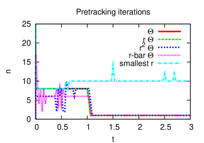
Figure 5: Number of pretracking iterations, which has the same cost as the same number of AH searches, for different pretracking methods at different times. The pretracking accuracy was $\Delta p=10^{-4}$; this means that the value $p^{*}$ of the pretracking surfaces at each time is only accurate up to this error (see section III.3).

IV.2 Coalescing Black Holes with Angular Momentum

As a further application for pretracking we consider an inspiralling black hole setup. We emphasise that pretracking is of high importance in these cases, where the two black holes can stay apart for times of more than $100\,M$ (see e.g. Brügmann et al. (2004)). Pretracking provides valuable information about impending apparent horizon formation as well as the necessary initial guess for the apparent horizon finder, or it can (with some confidence) exclude that a common AH exists.

The model we consider is the innermost stable circular orbit as predicted in Baumgarte (2000), which applies the effective potential techniques of Cook (1994) to puncture initial data Brandt and Brügmann (1997). Previous simulations with this dataset suggest that they perform around a half orbit before a common horizon first appears Baker et al. (2002); Alcubierre et al. (2004). The initial data contain two punctures with a proper horizon separation of $L=4.99\,M$, angular momentum $J=0.78\,M^{2}$ and angular velocity $\Omega=0.17/M$, where $M$ is the ADM mass of the system. This dataset was studied in detail in Alcubierre et al. (2004). This model is the first in the sequence (QC-0) studied with the Lazarus perturbative matching technique in Baker et al. (2002). The QC-0 model is attractive as a test-bed for pretracking since a common apparent horizon is found at around $t=16.44\,M$, while the simulation continues accurately beyond $t=40\,M$.

In this model, an initial guess for the common apparent horizon with a spherical form will find the common AH at the same iteration as pretracking if the chosen radius is accurate to about 10%. For black hole simulations that start out with a larger separation, the initial guess usually has to be ellipsoidal in order to find the common AH at all. In that case, all axis lengths have to be guessed correctly to the above accuray.

The evolutions were performed in bitant symmetry, i.e., with a reflection symmetry about $z=0$ plane. We used a grid containing $256\times 256\times 128$ points and a resolution of $\Delta x=0.06\,M$, which places the outer boundary at only about $7.68\,M$ for this test run. The evolutions were stopped at $t=22\,M$ since we were not interested in further tracking the evolution of the common apparent horizon and its ring-down. During the evolution we used a co-rotation shift to keep the black holes from moving across the grid Brügmann et al. (2004); Alcubierre et al. , which is essential for long-term stable evolutions. We used a $1+\log$ slicing and a $\Gamma$-driver shift condition Alcubierre et al. (2003).

Figure 6 shows the evolution of the pretracking surfaces found by different algorithms. The upper left plot shows the various pretracking surfaces at the initial time. It is obvious that the different algorithms are locating very different surfaces. Note that the covariant method $r$-bar $\Theta$ has the most distorted shape. The bump in the waist of the $r^{2}\Theta$ surface at $t=5\,M$ and $t=10\,M$ is caused by insufficient resolution in the surface; our explicit $h(\theta,\phi)$ representation is not well adapted to a peanut-shaped surface. The surface evolution can still be tracked, however, and later approaches the correct AH shape.

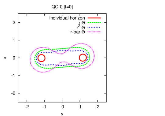
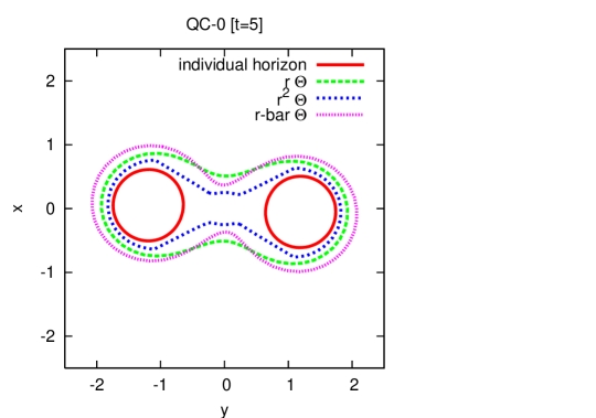
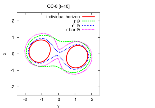
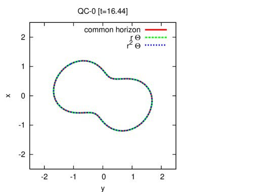
Figure 6: Time evolution of the different pretracking surfaces in the $xy$-plane for the inspiralling QC-0 model. Shown are individual and common apparent horizons and the pretracking surfaces found using different pretracking algorithms. A common horizon first appears at $t=16.44M$, shown in the lower right plot. It does not show the $r$-bar $\Theta$ surface because it could not be found at that time.

After $t=12.75\,M$, the method $r$-bar $\Theta$ fails to locate a surface. It succeeds again at $t=16.79\,M$, but it has then locked onto a surface that is inside the AH. We assume that this is due to the larger coordinate distortion of this surface, which has a much more pronounced waist than the other methods. The individual horizons are lost after $t=14.34\,M$. At $t=16.44\,M$ a common apparent horizon is found for the first time. The lower right hand graph compares different surfaces at that time and demonstrates that the succeeding pretracking methods have converged to the same surface.

Figure 7 shows the average expansions and the areal radii of the pretracking surfaces. The time at which the common AH is found is marked with a vertical line. The different pretracking methods track different surfaces during most of the evolution, but these surfaces converge about $1.5\,M$ before the common AH is found. The pretracking surfaces approach the common apparent horizon smoothly, and they accurately predict both its shape and its area. Pretracking gives here an early indication of the time at which the common AH forms. After the common AH has formed, the pretracking methods $r\Theta$ and $r^{2}\Theta$ lock onto the AH. The method $r$-bar $\Theta$, which failed to locate a surface for some time, afterwards tracks a different surface. Both methods $r\Theta$ and $r^{2}\Theta$ are thus reliable pretracking methods for this evolution.

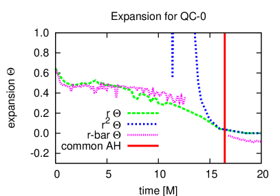
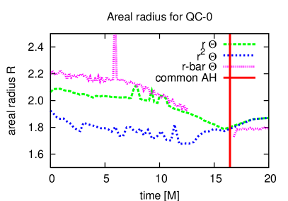
Figure 7: Average expansion $\Theta$ and areal radius $R$ for the inspiralling black hole evolution. The average expansion for $r^{2}\Theta$ is larger than can be shown on this scale. This is due to numerical errors, as explained in the main text. The method $r$-bar $\Theta$ fails after $t=12.75\,M$; it succeeds again after the common AH has formed, but tracks a surface that is not the AH.

We measured the angular momentum of the pretracking surfaces using the dynamical horizon framework Ashtekar and Krishnan (2004); our implementation is described in Dreyer et al. (2002). We show the results in Fig. 8. Note that this angular momentum measure is a quasi-local quantity and therefore is defined on any surface, not only apparent horizons. However, our current implementation is restricted to cases that are close to having an axial Killing vector. In dynamical spacetimes this condition will only be satisfied approximately. Yet in the case of this merger simulation both successful pretracking methods $r\Theta$ and $r^{2}\Theta$ predict the angular momentum of the common apparent horizon.

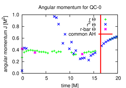
Figure 8: Angular momentum $J$ of the pretracking surfaces versus time, measured with the dynamical horizon framework. The angular momentum of the common AH increases directly after it has formed, indicating that it accretes both energy and angular momentum initially. In the few cases where a value for $J$ could be found for the $r$-bar $\Theta$ pretracking surfaces, they agree well with the $r\Theta$ method. In some cases, no angular momentum could be measured because no approximate Killing vector could be found on the pretracking surface at that time.

We conclude that pretracking works as an effective analysis tool for this binary black hole collision. The time of merger is predicted by the rate in which the expansion of the pretracking surfaces approaches zero, and the pretracking surfaces give a good estimate for the shape, area, and angular momentum for the future common apparent horizon.

V Conclusion

Horizon pretracking is an effective method for predicting the location and shape of an emerging common horizon, as well as yielding important physical information during the course of a spacetime evolution. The simple cases tested here indicate that it is applicable to a variety of scenarios, such as black hole mergers, where the formation of a horizon is expected, but its location and shape are not known a priori.

Various practical issues need to be taken into consideration when choosing an appropriate surface family for pretracking. A family of CE surfaces parametrised by their expansion suffers some drawbacks, since the expansion does not increase monotonically. However, a simple modification such as the multiplication by a coordinate radius leads to an effective practical algorithm. We have shown that several methods for defining the pretracking surface all lead to procedures which accurately determine the common AH at the time of its first formation.

As the lifetimes of black hole evolutions with dynamic gauges are extended, this ability to predict the common horizon shape will become particularly important. Apparent horizon finders require a reasonable initial guess in order to converge. After a long period of evolution of separated black holes, the initial common horizon shape is difficult to predict. As a result, a common AH may not be found, or at least not at the earliest possible moment. This can lead to the impression that one is evolving separated black holes when they have actually already merged. Valuable physical information, which can be determined from the shape and oscillations of the common horizon, will be lost. On a practical level, finding the earliest common AH gives important information as to the causality of the spacetime and allows more effective application of certain numerical techniques, such as singularity excision.

We observe that new trapped surfaces form in pairs of an outer and an inner surface. A given initial guess for the horizon surface will find only one of these surfaces, which tend to diverge quickly in coordinate space. Since initially they are identical, however, an AH finding algorithm will converge to either the inner or the outer depending on its initial guess. This is particularly true if the common AH is found very early (as is the intention of the pretracking method). We have given a simple algorithm that helps selecting the outer, generally less distorted surface, which is the astrophysically interesting apparent horizon. This algorithm does not depend on pretracking and is useful in general.

We emphasise here that valuable information can be gained from the study of foliations of CE (and related) surfaces in a slice, beyond the commonly studied apparent horizons. The dynamical horizon formalism defines a quasi-local measure of the spin that can be evaluated on any closed surface, and the three-covariantly defined CE surfaces form a natural choice. Gauge conditions can also be designed to reduce distortions in such surfaces, or hold them in place on the grid, potentially simplifying the dynamics.

The pretracking method is efficient enough to be applied as a regular analysis tool during large simulations. It is already being used in a variety of simulations of binary puncture and thin sandwich data evolutions, and is finding further application in hydrodynamical collapse scenarios.

Appendix A Expressions for the Jacobians

We list here for the reader’s convenience the equations and Jacobians for the pretracking methods that we use in this paper. See table 1 for the combinations of shape and goal functions and the names that we use for these combinations.

We assume that a desired goal function value $p$ is given, and a corresponding surface $h$ is to be determined by the combination of the shape and the goal function. For all methods, we list first the system of equations that defines the surface, and then give the Jacobian of this system. The intermediate quantity $C$ is also determined through these equations, but its value is irrelevant.

We denote the expansion of the surface $h$ with $\Theta_{i}$, and the expansion’s Jacobian as $J_{ij}=\partial\Theta_{i}/\partial h_{j}$. These expressions are e.g. given in Schnetter (2003) or Thornburg (2004). $\delta_{ij}$ is the Kronecker delta symbol.

Method $\Theta$:

shape function $H_{1}$, goal function $G_{H}$:

$$\Theta_{i}-C = 0$$ (19)

$$C-p = 0$$

$$\left(\begin{array}[]{c|c}\displaystyle J_{ij}&\displaystyle-1\\ \hline\cr\displaystyle 0&\displaystyle+1\end{array}\right)$$ (20)

Method $r\Theta$:

shape function $H_{r}$, goal function $G_{H}$:

$$\Theta_{i}h_{i}-C = 0$$ (21)

$$C-p = 0$$

$$\left(\begin{array}[]{c|c}\displaystyle J_{ij}h_{i}+\Theta_{i}\delta_{ij}&\displaystyle-1\\ \hline\cr\displaystyle 0&\displaystyle+1\end{array}\right)$$ (22)

Method $r^{2}\Theta$:

shape function $H_{r^{2}}$, goal function $G_{H}$:

$$\Theta_{i}h_{i}^{2}-C = 0$$ (23)

$$C-p = 0$$

$$\left(\begin{array}[]{c|c}\displaystyle J_{ij}h_{i}^{2}+2\Theta_{i}h_{i}\delta_{ij}&\displaystyle-1\\ \hline\cr\displaystyle 0&\displaystyle+1\end{array}\right)$$ (24)

Method $r$-bar $\Theta$:

shape function $H_{1}$, goal function $G_{Hr}$:

$$\Theta_{i}-C = 0$$ (25)

$$C-\frac{1}{N}\sum_{k}\Theta_{k}+\frac{1}{N}\sum_{k}\Theta_{k}\cdot\frac{1}{N}\sum_{k}h_{k}-p = 0$$

$$\left(\begin{array}[]{c|c}\displaystyle J_{ij}&\displaystyle-1\\ \hline\cr\displaystyle-\frac{1}{N}\sum_{k}J_{kj}+\frac{1}{N}\sum_{k}J_{kj}\cdot\frac{1}{N}\sum_{k}h_{k}+\frac{1}{N}\sum_{k}\Theta_{k}\cdot\frac{1}{N}&\displaystyle+1\end{array}\right)$$ (26)

Method smallest $r$:

shape function $H_{1}$, goal function $G_{r}$:

$$\Theta_{i}-C = 0$$ (27)

$$C-\frac{1}{N}\sum_{k}\Theta_{k}+\frac{1}{N}\sum_{k}h_{k}-p = 0$$

$$\left(\begin{array}[]{c|c}\displaystyle J_{ij}&\displaystyle-1\\ \hline\cr\displaystyle-\frac{1}{N}\sum_{k}J_{kj}+\frac{1}{N}&\displaystyle+1\end{array}\right)$$ (28)

Method inner $r\Theta$:

same as $r\Theta$ above

References

- Ashtekar and Krishnan (2004) A. Ashtekar and B. Krishnan, Living Rev. Rel. 7, 10 (2004), eprint gr-qc/0407042.
- Dreyer et al. (2002) O. Dreyer, B. Krishnan, D. Shoemaker, and E. Schnetter, Phys. Rev. D 67, 024018 (2002), eprint gr-qc/0206008.
- Cook et al. (1998) G. B. Cook, M. F. Huq, S. A. Klasky, M. A. Scheel, A. M. Abrahams, A. Anderson, P. Anninos, T. W. Baumgarte, N. Bishop, S. R. Brandt, et al., Phys. Rev. Lett 80, 2512 (1998).
- Alcubierre et al. (2001) M. Alcubierre, B. Brügmann, D. Pollney, E. Seidel, and R. Takahashi, Phys. Rev. D 64, 061501(R) (2001), eprint gr-qc/0104020.
- Anninos et al. (1995a) P. Anninos, G. Daues, J. Massó, E. Seidel, and W.-M. Suen, Phys. Rev. D 51, 5562 (1995a).
- Balakrishna et al. (1996) J. Balakrishna, G. Daues, E. Seidel, W.-M. Suen, M. Tobias, and E. Wang, Class. Quantum Grav. 13, L135 (1996).
- (7) M. Alcubierre, P. Diener, F. S. Guzmán, S. Hawley, M. Koppitz, D. Pollney, and E. Seidel, in preparation.
- Anninos et al. (1995b) P. Anninos, D. Hobill, E. Seidel, L. Smarr, and W.-M. Suen, Phys. Rev. D 52, 2044 (1995b).
- Hawking and Ellis (1973) S. W. Hawking and G. F. R. Ellis, The Large Scale Structure of Spacetime (Cambridge University Press, Cambridge, England, 1973).
- Thornburg (1987) J. Thornburg, Class. Quantum Grav. 4, 1119 (1987), URL http://stacks.iop.org/0264-9381/4/1119.
- Seidel and Suen (1992) E. Seidel and W.-M. Suen, Phys. Rev. Lett. 69, 1845 (1992).
- Thornburg (1996) J. Thornburg, Phys. Rev. D 54, 4899 (1996), eprint gr-qc/9508014.
- Schnetter (2003) E. Schnetter, Class. Quantum Grav. 20, 4719 (2003), eprint gr-qc/0306006, URL http://stacks.iop.org/0264-9381/20/4719.
- Thornburg (2004) J. Thornburg, Class. Quantum Grav. 21, 743 (2004), eprint gr-qc/0306056, URL http://stacks.iop.org/0264-9381/21/743.
- Anninos et al. (1998) P. Anninos, K. Camarda, J. Libson, J. Massó, E. Seidel, and W.-M. Suen, Phys. Rev. D 58, 24003 (1998).
- Metzger (2004) J. Metzger, Class. Quantum Grav. 21, 4625 (2004), eprint gr-qc/0408059, URL http://stacks.iop.org/CQG/21/4625.
- Shoemaker et al. (2000) D. M. Shoemaker, M. F. Huq, and R. A. Matzner, Phys. Rev. D 62, 124005 (2000).
- Huisken and Yau (1996) G. Huisken and S.-T. Yau, Invent. Math. 124, 281 (1996).
- Shapiro and Teukolsky (1985) S. L. Shapiro and S. A. Teukolsky, Astrophys. J. 298, 58 (1985).
- Bishop (1982) N. T. Bishop, Gen. Rel. Grav. 14, 717 (1982).
- Cook and Abrahams (1992) G. B. Cook and A. M. Abrahams, Phys. Rev. D 46, 702 (1992).
- Nakamura et al. (1987) T. Nakamura, K. Oohara, and Y. Kojima, Prog. Theor. Phys. Suppl. 90, 1 (1987).
- Shibata and Nakamura (1995) M. Shibata and T. Nakamura, Phys. Rev. D 52, 5428 (1995).
- Baumgarte and Shapiro (1999) T. W. Baumgarte and S. L. Shapiro, Phys. Rev. D 59, 024007 (1999), eprint gr-qc/9810065.
- Alcubierre et al. (2003) M. Alcubierre, B. Brügmann, P. Diener, M. Koppitz, D. Pollney, E. Seidel, and R. Takahashi, Phys. Rev. D 67, 084023 (2003), eprint gr-qc/0206072.
- Brandt and Brügmann (1997) S. Brandt and B. Brügmann, Phys. Rev. Lett. 78, 3606 (1997), eprint gr-qc/9703066.
- (27) Cactus, http://www.cactuscode.org.
- Brill and Lindquist (1963) D. Brill and R. Lindquist, Phys. Rev. 131, 471 (1963).
- Brügmann et al. (2004) B. Brügmann, W. Tichy, and N. Jansen, Phys. Rev. Lett. 92, 211101 (2004), eprint gr-qc/0312112.
- Baumgarte (2000) T. W. Baumgarte, Phys. Rev. D 62, 024018 (2000), eprint gr-qc/0004050.
- Cook (1994) G. B. Cook, Phys. Rev. D 50, 5025 (1994).
- Baker et al. (2002) J. Baker, M. Campanelli, C. O. Lousto, and R. Takahashi, Phys. Rev. D 65, 124012 (2002), eprint [http://arXiv.org/abs]astro-ph/0202469.
- Alcubierre et al. (2004) M. Alcubierre, B. Brügmann, P. Diener, F. S. Guzmán, I. Hawke, S. Hawley, F. Herrmann, M. Koppitz, D. Pollney, E. Seidel, et al., submitted to Phys. Rev. D (2004), eprint gr-qc/0411149.