Gauge pathologies in singularity-avoidant spacetime foliations

Abstract

The family of generalized-harmonic gauge conditions, which is currently used in Numerical Relativity for its singularity-avoidant behavior, is analyzed by looking for pathologies of the corresponding spacetime foliation. The appearance of genuine shocks, arising from the crossing of characteristic lines, is completely discarded. Runaway solutions, meaning that the lapse function can grow without bound at an accelerated rate, are instead predicted. Black Hole simulations are presented, showing spurious oscillations due to the well known slice stretching phenomenon. These oscillations are made to disappear by switching the numerical algorithm to a high-resolution shock-capturing one, of the kind currently used in Computational Fluid Dynamics. Even with these shock-capturing algorithms, runaway solutions are seen to appear and the resulting lapse blow-up is causing the simulations to crash. As a side result, a new method is proposed for obtaining regular initial data for Black Hole spacetimes, even inside the horizons.

I Introduction

The choice of a coordinate system is mandatory when finding solutions of Einstein’s field equations. In the 3+1 approach ADM , this choice can be made in two steps:

• The choice of a time coordinate. In geometrical terms, this amounts to select a specific foliation of spacetime by a family of spacelike hypersurfaces (the constant time slices).

• The choice of the space coordinates. In geometrical terms, this amounts to select a specific congruence of lines threading every slice of the time foliation (the time lines).

Most of the theoretical developments in the 3+1 approach are space-invariant, that is independent of the choice of the space coordinates. In this case, one can safely select as time lines precisely the normal lines to the time slices (normal coordinates), as we will do in what follows. In local adapted coordinates, we will write then the line element as

$$ds^{2}=-\alpha^{2}~{}dt^{2}+\gamma_{ij}~{}dx^{i}~{}dx^{j}\,.$$ (1)

The choice of a time coordinate, however, is not so simple. In numerical simulations one must care about physical singularities that could arise dynamically in gravitational collapse scenarios. Care must be taken to avoid the time slices to hit the singularity in a finite amount of coordinate time: otherwise the numerical code will crash due to the singular terms.

This is why singularity avoidant slicing conditions are widely used in Numerical Relativity. A first example is provided by the maximal slicing condition,

$${\rm tr}\,K=0\,,$$ (2)

where

$$K_{ij}=-\frac{1}{2\alpha}~{}\partial_{t}~{}\gamma_{ij}$$ (3)

is the extrinsic curvature tensor of the time slices. Maximal slicing has been successfully used in Black Hole simulations since the early times SY78 . The behavior of maximal slicing in simple cases has been studied for more than thirty years Eetal73 and is still being studied today Reimann04 . The problem with maximal slicing is that it leads to a second order elliptic equation for the lapse function $\alpha$. This can be a complication in the current 3D simulations, where the need of accuracy is consuming all the available computational resources. But this is also a complication from the theoretical point of view, because the resulting evolution system (field equations plus coordinate conditions) is then of a mixed elliptic-hyperbolic type.

A simpler alternative is provided by the generalized harmonic condition BM95

$$\partial_{t}~{}\alpha=-f\alpha^{2}~{}{\rm tr}\,K\,,$$ (4)

where $f$ can be an arbitrary function of $\alpha$ ($f=1$ in the original harmonic slicing CR83 ; BM88 ). It provides a first order evolution equation for the lapse function which, when combined with the field equations, leads to a hyperbolic evolution system (weakly hyperbolic or strongly hyperbolic, depending on the formulation) for non-negative choices of $f$.

The problem with condition (4) is that it can lead to gauge-related pathologies. In Ref. AMSST95 , this has been seen to occur in Black Hole simulations for some particular cases. In Ref. Alcubierre97 , the generic case is considered; starting from an analysis of the characteristic speeds, the conclusion is that there can be two classes of shocks:

• one which affects just the gauge degrees of freedom. A cure is suggested, consisting in the choice

  $$f=1+k/\alpha^{2}$$ (5)

  ($k$ being just an integration constant).

• another one which affects even the metric degrees of freedom (with $c$ as characteristic speed), for which there is no cure.

The claim concerning the existence of gauge shocks has been recently strengthened Alcubierre03 by providing a purely kinematical derivation of the condition (5), independently of the field equations.

These are by no means rhetorical questions. We are aware that Einstein’s equations can be used for describing the propagation of discontinuities arising either from the initial or the boundary data. We are talking here about something stronger: shocks that could arise dynamically even from smooth initial and boundary data. This is a well known phenomenon in the Fluid Dynamics domain: the non-linearity of the equations leads in some circumstances to the crossing of the characteristic lines so that a genuine shock (not just a contact discontinuity) appears. Can this really happen in General Relativity?. Or, at least, can this happen when using (4) as slicing condition?. We think that this is a good opportunity to address these questions and provide, as far as possible, definite answers.

II Are there metric shocks?

No, there are not metric shocks. To see why, let us start with the space-invariant expression of the corresponding characteristic speed (light speed)

$$c=\frac{dl}{dt}=\sqrt{\gamma_{ij}~{}\frac{dx^{i}}{dt}~{}\frac{dx^{j}}{dt}}=\pm~{}\alpha$$ (6)

(length variation per unit coordinate time). We can always consider a geodesic slicing, so that $\alpha=1$ and coordinate time coincides with proper time. In this case, as depicted in Fig. 1, the characteristic lines (light rays) along any given space direction can not even approach one another.

The question is whether these light rays can cross each other in some alternative slicing. As shown in Fig. 1, this can never happen as long as the time slices are spacelike hypersurfaces. Without characteristic crossing, there are not genuine shocks (although contact discontinuities can appear from initial or boundary data, as discussed in the Introduction). Einstein’s field equations can then be said to be, in the Applied Mathematics jargon, linearly degenerate. The case of the gauge degrees of freedom, which are not prescribed by the field equations, will be discussed in the following sections.

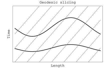
Figure 1: The diagram shows a set of light rays as straight lines with unit slope in a time-length diagram (geodesic slicing). Two hypersurfaces (time slices) of an alternative slicing are also shown. These hypersurfaces must be spacelike, so that the slope of the tangent vectors is limited by that of the light rays. Notice that the space distance among light rays, as measured on the time slices, is no longer constant. But notice also that the order of the sequence of light rays on each time slice is unaltered.

But let us look back before at Ref. Alcubierre97 , where a coordinate-dependent expression for light speed was used as the starting point. If we repeat the arguments of Ref. Alcubierre97 , but using instead the space-invariant expression (6) as the starting point, we see that the prediction of metric shocks disappears. The prediction of gauge shocks remains, but condition (5) for the proposed cure is to be replaced by

$$f=k/\alpha^{2}\,,$$ (7)

which no longer contains the original harmonic slicing ($f=1$) as a particular case.

III Is there a kinematical reason for gauge shocks?

No, there is no kinematical reason for gauge shocks. The argument in Ref. Alcubierre03 starts from the time-slicing equation

$$\left[g^{\mu\nu}+(1-\frac{1}{f})~{}\frac{d^{\mu}\phi~{}d^{\nu}\phi}{(-g^{\rho\sigma}d_{\rho}\phi~{}d_{\sigma}\phi)}\right]~{}\nabla_{\mu}d_{\nu}\phi=0\,,$$ (8)

which reduces to the generalized harmonic slicing condition (4) in local adapted coordinates, where

$$\phi=t\,,\qquad\alpha=(-g^{\rho\sigma}d_{\rho}\phi~{}d_{\sigma}\phi)^{-1/2}\,.$$ (9)

The argument proceeds then by transforming the quasilinear second-order equation (8) into a first order system and studying the characteristic speeds, without recourse to the field equations Alcubierre03 .

We will take here a more direct approach, looking for the characteristic hypersurfaces of the original equation (8). To simplify the analysis, we will adapt the general coordinates in (8) to the (generic) initial data. Starting from a given spacelike slice $\Sigma$, we will choose then as initial conditions

$$\phi\mid_{\Sigma}=t_{0}\,,\qquad\partial_{k}\,\phi\mid_{\Sigma}=0\,,\qquad\partial_{t}\,\phi\mid_{\Sigma}=\alpha\,.$$ (10)

Notice that this is by no means a restriction on the initial data: it is rather the result of adapting the arbitrary spacetime coordinates to any specific choice of initial data. Moreover, this kind of adapted coordinates is precisely the one that is currently used in numerical simulations, where the equation (8) is always used in the form (4).

It is trivial now to look for the characteristic hypersurfaces. All second partial derivatives on $\Sigma$ can be obtained from (10) with the only exception of the second time derivative, which can be obtained from (8) unless

$$\frac{1}{f}~{}g^{00}\mid_{\Sigma}=0\,,$$ (11)

which would then imply that $\Sigma$ is a characteristic hypersurface. For any finite choice of $f$, condition (11), which can be written in an invariant way as

$$g^{\mu\nu}\partial_{\mu}\phi\,\partial_{\nu}\phi\mid_{\Sigma}=0\,,$$ (12)

amounts to the statement that $\Sigma$ is a null hypersurface. This means that the characteristic speed coincides again with light speed. It follows that the discussion of the preceding section applies here again to show that there can not be any crossing of characteristics and hence no genuine shocks can develop.

To put it in a different way: equation (8) can always be used for constructing a new foliation in a given (regular) spacetime provided that the resulting slices remain spacelike. Then, the time slicing itself will be well defined, although the behavior of the gauge-related dynamical fields may depend on the field equations, as we will see below.

IV Are there dynamical gauge shocks?

There are certainly gauge pathologies of a dynamical origin, but not genuine shocks. In order to analyze this point, it is convenient to consider the time derivative of the generalized harmonic slicing condition (4). This requires using the field equations to provide the time evolution of ${\rm tr}\,K$ (the arguments in this section will be then of a dynamical nature).

We will choose for simplicity the BSSN formulation SN95 ; BS99 , although all the current formalisms share the same physical solutions. In the vacuum case, we get after some algebra

$$(1/\tilde{f})~{}\partial_{tt}~{}\alpha-\triangle~{}\alpha=-~{}[~{}\alpha~{}{\rm tr}\,(K^{2})-\tilde{f}^{\prime}~{}({\rm tr}\,K)^{2}~{}]\,,$$ (13)

where we have noted for short

$$\tilde{f}\equiv f~{}\alpha^{2}\,,\qquad\tilde{f}^{\prime}\equiv\frac{\partial\,\tilde{f}}{\partial\,\alpha}\,.$$ (14)

Equation (13) can be interpreted as a generalized wave equation for the lapse function. The left-hand-side terms correspond to the principal part, and it is clear that the characteristic speed is given by

$$v_{G}=\pm\sqrt{f}\,\alpha$$ (15)

(gauge speed). We derived condition (7) by using precisely (15) as the starting point for the argument presented in Ref. Alcubierre97 : it amounts to the requirement of a constant gauge speed, that is

$$v_{G}={\rm constant}~{}\Leftrightarrow~{}\tilde{f}^{\prime}=0\,.$$ (16)

The right-hand-side terms in (13) can be interpreted as non-linear source terms for the evolution of the lapse function. Allowing for (4), ${\rm tr}\,K$ is proportional to the time derivative of $\alpha$, so that there is a non-linear coupling that can lead to runaway (growing without bound, at an increasing rate) solutions.

An extreme example of this gauge pathology, in which transport plays not role at all, is provided by space-homogeneous and isotropic solutions, like the ones used in Cosmology, where all space derivatives vanish and the extrinsic curvature is proportional to the metric. One has then

$$\partial_{tt}~{}\alpha=\tilde{f}\,(\tilde{f}^{\prime}-\frac{\alpha}{3})\,({\rm tr}\,K)^{2}=\frac{1}{\tilde{f}}\,(\tilde{f}^{\prime}-\frac{\alpha}{3})\,(\partial_{t}\,\alpha)^{2}\,,$$ (17)

so that $\alpha$ can grow without bound, with a driving force proportional to the square of the growing rate, unless

$$\tilde{f}^{\prime}\leq\frac{\alpha}{3}\qquad\Leftrightarrow\qquad f=n+\frac{k}{\alpha^{2}}\qquad(n\leq\frac{1}{6})\,.$$ (18)

Coming back to the general case, it is clear that condition (16) could be interpreted in two alternative ways

• Ensuring a constant gauge speed, so that no characteristic crossing can occur.

• Ensuring the negative sign of the source terms in (13), so that no runaway solutions can occur.

This ambiguity follows from the very nature of the argument proposed in Ref. Alcubierre97 , where the main idea is to include the source terms in the discussion about the behavior of characteristic fields. The $\tilde{f}$-dependent term in the right-hand-side of (13) would then be considered as a non-linear contribution to the transport (left-hand-side) terms.

But we do not see much difference between this particular quadratic term and the other ones in the right-hand-side of (13), independently of their origin. The example we presented before shows instead how these other source terms actually contribute to the regularity condition (18) by providing an upper bound which was missing in (16).

Our conclusion is that any pathological behavior of the gauge-dependent degrees of freedom, which manifests itself as an unbounded growth of either the lapse function or its first derivatives, can be interpreted consistently as the effect of the non-linear source terms in the evolution equations. We will test this conclusion against simple numerical Black-Hole simulations in what follows.

V Gauge pathologies in numerical Black-Hole simulations

We will focus here on three-dimensional numerical simulations of a spherically symmetric Black Hole. As far as we are interested in the strong field region, the Black Hole interior is not excised from the numerical grid. Regular initial data are obtained by using a novel ’Free Black Hole’ approach, which relies on the well known ’no hair’ theorems (see Appendix I for details). This new approach is also being applied independently in the context of the BSSN formalism Denis .

We will use in our simulations the first order version of the Z4 evolution formalism Z4 ; Z48 in normal coordinates (zero shift). Apart from standard centered finite-difference algorithms, we will use at some point the MMC method. This is a high-resolution shock-capturing (HRSC) method which combines the monotonic-centered (MC) flux limiter vanLeer77 with Marquina’s flux formula Marquina (see Appendix II for details). The use of these advanced HRSC methods is also new in 3D Black Hole simulations, although it is crucial for our arguments about shocks.

V.1 Slice stretching

Figure 2: Lapse collapse for the ’1+log’ slicing : the lapse values are shown every $0.5M$. The lapse gets very close to zero in the innermost region. A standard finite difference algorithm is used in a cubic cartesian grid (the space direction in the plots corresponds to the grand diagonal of the cube). Spurious oscillations appear at about $t=6M$ in the zones where the slope is changing more abruptly.

The first stages of the simulation show a collapse of the space volume element which, allowing for the singularity avoidance properties of the gauge conditions (4), translates itself into a collapse of the lapse function $\alpha$. This lapse collapse can be slower or faster, depending on our choice of $f$. We will present here our results for the ’1+log’ case

$$f=\frac{2}{\alpha}\,,$$ (19)

although no qualitative difference is detected for similar choices, like $f=2$ for instance.

Figure 3: Plots of $K_{xx}$ (solid line) and ${\rm tr}\,K$ (dotted line) along the $x$ axis, corresponding to the 1+log slicing at $t=6M$. Negative values of $K_{xx}$ correspond to the increasing of $\gamma_{xx}$, that is a radial stretching of the time slice. Notice that this is compatible with an overall collapse pattern, as shown by the positivity of ${\rm tr}\,K$: the radial stretching is then compensated by the collapse along the angular directions. The profile of ${\rm tr}\,K$ is smooth, without any sign of shocks.

Figure 4: Same as Figure 2, but using the MMC numerical algorithm for the space discretization, as described in Appendix II. The spurious oscillations have completely disappeared. Slice stretching is still there (Figure 3 corresponds actually to the last plot), but it is no longer a problem for numerical simulations.

Let us see what happens after some time. We see in Fig. 2 how high-frequency oscillations start appearing in the regions where the lapse slope is changing more abruptly. This is a numerical effect: it is the analogous of the well-known Gibbs phenomenon, which appears when the tool one is using (the standard finite difference method in our case) is unable to resolve the higher frequency modes of some dynamical field.

In order to see where those annoying high-frequency modes came from, let us take a look at behavior of the extrinsic curvature, as displayed in Fig. 3. What we see there is the well known ’slice stretching’ phenomenon: the Black Hole is sucking both the numerical grid ST86 ; ADMSS95 and the space slice Reimann04 ; RB04 , producing as a result steep profiles along the radial direction. High-frequency modes are the expected to appear in the regions with abrupt slope changes in some dynamical field.

The same kind of spurious oscillations currently appears in Computational Fluid Dynamics simulations, in regions where genuine shocks are developing. The cure is to use advanced HRSC numerical methods that can deal with shocks without altering the monotonicity of the dynamical fields. We will use in what follows the MMC numerical algorithm, as described in Appendix II, which is one of such HRSC methods. We are aware that we are not dealing here with real shocks (the ${\rm tr}\,K$ profile in Fig. 3 is clearly smooth). We are instead dealing with, let us say, ’numerical shocks’ as far as our numerical grid is just unable to resolve the higher frequency modes associated with slice stretching.

The effect of switching to the MMC numerical method is definitive, as it can be seen on Fig. 4. No trace of the spurious oscillations remains. There is nothing either in the lapse or in the ${\rm tr}\,K$ profiles that could be interpreted as a shock. The conclusion is obvious: slice stretching does not produce any real shock, it may produce just ’numerical shocks’ that disappear when improving the discretization algorithm.

V.2 Runaway solutions

Let us see now what happens when allowing our simulations to proceed for a longer time (about $t=14M$ in our case, but the value will depend on the specific gauge choice). We see in Fig. 5 that the spurious oscillations do not show up anymore. What we see instead is a sort of rebound of the lapse, which is the prelude of a blow up that will crash the numerical simulation. We have stopped the simulation in Fig. 5 before the crash occurs, so that two different interpretations can be tentatively considered

• A gauge shock is forming and starts propagating backwards in the region near to $\rho=2M$.

• The growing of the lapse is triggering a runaway solution that will result in a lapse blow up.

Figure 5: Same as Figure 4, but with the simulations running up to $t=14M$. No spurious oscillations appear anymore. However, the lapse collapse stops and a sort of rebound starts near the frozen innermost region. The lapse looks just going backwards there. The simulation is going to crash by a lapse blow up.

In order to discriminate between these two alternatives, let us take a look to Fig. 6, where we have plotted the same extrinsic curvature components as in Fig. 3. As a word of caution, let us remember that the lapse in the innermost region is yet collapsed, so that the dynamics is frozen there. This means that the features we see in the innermost region in Fig. 6 correspond to an earlier stage (measured in proper time) than what we see around $\rho=2M$, which is the region we are going to analyze now.

Figure 6: Same as Fig. 3, but now for $t=14M$, corresponding to the last plot in Fig. 5. The dynamics in the innermost region is frozen (the lapse is fully collapsed there). In the region around $\rho=2M$, however, positive values of $K_{xx}$ appear, corresponding to a radial collapse, whereas ${\rm tr}\,K$ becomes negative, corresponding to a global expansion pattern. This is just the behavior opposite to slice stretching, and it explains the lapse rebound that can be seen in Fig. 5. Notice that the collapse pattern (positive $trK$ values) is recovered in the outermost region, where the lapse collapse proceeds as expected.

What we see there is just the opposite that what we saw in Fig. 3: ${\rm tr}\,K$ is now negative, so that we have an overall expansion pattern. But the radial component ($K_{xx}$ along the $x$ direction) is collapsing. This explains why the whole picture in Fig. 5 looks like moving backwards in time in the rebounding region.

Notice that the ${\rm tr}\,K$ profile in Fig. 6 is clearly smooth and well-resolved in the region around $\rho=2M$, so that the shock interpretation can be excluded. Moreover, as far as we are using a HRSC numerical method, no blow up would be expected from the presence of shocks. In Computational Fluid Dynamics these methods are currently used for dealing with genuine shocks without crashing because of that. The blow up must be actually caused by something much stronger than a mere shock: a runaway solution that is triggered by the negative values of ${\rm tr}\,K$, which correspond to an overall expansion behavior.

The appearance of runaway solutions is to be expected when selecting the ’1+log’ (19) or any similar choice among the singularity-avoidant family of slicing conditions (4). If we decompose the extrinsic curvature tensor $K_{ij}$ into its irreducible components

$$A_{ij}\equiv K_{ij}-\frac{{\rm tr}\,K}{3}~{}\gamma_{ij}\,,\qquad K\equiv{\rm tr}\,K$$ (20)

(shear tensor and expansion factor, respectively), we see that the source terms in the lapse equation (13) can be expressed as

$$-\alpha~{}({\rm tr}\,A^{2})+(2-\frac{\alpha}{3})~{}K^{2}\,,$$ (21)

which can easily get a positive sign in collapsing scenarios ($\alpha$ small) unless the expansion factor $K$ is kept to low values when compared with the shear tensor.

We conclude that runaway solutions, not gauge shocks, can be a real problem in simulations that, like in the Black Hole cases, make use of the singularity-avoidant slicing conditions (4). To find a convenient cure for this gauge pathology (excising the interior region, using a dynamical shift, selecting other values of $f$, and so on) goes beyond the purpose of this paper.

Appendix I: Free Black Hole initial data

Based in the idea that the interior region of a Black Hole has no causal physical influence on the exterior one (no-hair theorems), we can devise a simple way of obtaining regular initial data for Black Hole spacetimes:

• Solve the energy and momentum constraints for the initial data. This currently leads to a singular space metric.

• Replace the metric in the interior regions by any smooth extension of the exterior geometry. Energy and momentum constraints will be no longer fulfilled inside the horizons (’Free Black Hole’ data).

In the simplest case, we can consider time-symmetric vacuum initial data with a conformally flat space metric, that is

$$K_{ij}\mid_{t=0}~{}=~{}0\,,\qquad\gamma_{ij}\mid_{t=0}~{}=~{}\Psi^{4}~{}\delta_{ij}\,,$$ (I.1)

so that the momentum constraint is trivially satisfied and the energy constraint amounts to require that $\Psi$ be an harmonic function of the Euclidean metric.

Free initial data can be obtained then for a spherically symmetric Black Hole with mass $M$ by starting from the singular conformal factor

$$\Psi=1+\frac{M}{2\rho}\,,$$ (I.2)

and replacing its value inside the horizon (dotted line in Fig. 7) by any smooth function (continuous line in Fig. 7).

Figure 7: Plot of a conformal factor $\Psi$ providing time-symmetric conformally-flat initial data for a free Schwarzschild Black Hole. Values on the $x$ axis correspond to the isotropic radial coordinate $\rho$, measured in units of $M$. The singular solution in the interior region (dashed line) is replaced by a regular one (continuous line). Both expressions coincide in the exterior region. Notice that the matching is smooth at the apparent horizon ($\rho=M/2$).

In the Z4 formalism, energy and momentum constraint violations will cause the growing of the supplementary fields $\Theta$ and $Z_{k}$, which non-zero values correspond to a departure of true Einstein’s solutions. But these fields, which are the 3+1 components of the four-vector $Z_{\mu}$ are known to verify Z4

$$\Box Z_{\mu}+R_{\mu\nu}Z^{\nu}=0\,,$$ (I.3)

so that the spurious non-zero values propagate with light speed. The exterior geometry, then, can not be affected by constraint violations inside the horizon (at least not at the continuum level).

Appendix II: The MMC high-resolution method

High-Resolution Shock-Capturing (HRSC) numerical methods can be applied to strongly-hyperbolic first-order systems of balance laws. The balance-law structure means that the evolution equations for the array $\mathbf{u}$ of dynamical fields can be written as

$$\partial_{t}~{}\mathbf{u}+\partial_{k}~{}\mathbf{F}^{k}=\mathbf{S}\,,$$ (II.1)

where both the Flux $\mathbf{F}^{k}$ and the Source $\mathbf{S}$ terms depend algebraically on the fields, but not on their derivatives:

$$\textbf{F}^{k}=\textbf{F}^{k}(\textbf{u})\,,\qquad\textbf{S}=\textbf{S}(\textbf{u})\,.$$ (II.2)

The system (II.1) will be strongly hyperbolic if and only if for every space direction $\vec{n}$, the corresponding characteristic matrix

$$n_{k}\mathbf{A}^{k}=n_{k}\frac{\partial\mathbf{F}^{k}}{\partial\mathbf{u}}$$ (II.3)

has real eigenvalues $\mathbf{v}$ (characteristic speeds) and a complete set $\mathbf{w}$ of eigenvectors KL89 .

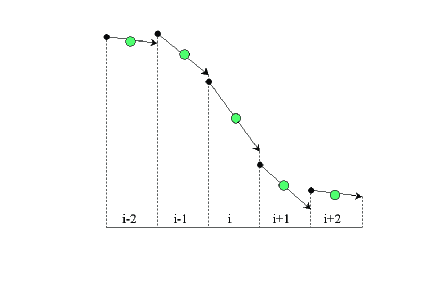
Figure 8: Starting from the values of the fluxes at the grid nodes, a linear reconstruction is done inside every elementary cell. Numerical discontinuities appear at every interface (dotted lines) between the left and right values (arrows and dots, respectively). Notice that the original function was monotonically decreasing: all the slopes are negative. In the proposed reconstruction, however, both the left interface sequence (at $i-3/2$) and the right interface one (at $i+3/2$) show local extreme values that break the monotonicity of the original function.

The balance law form (II.1) is specially suited for the method-of-lines (MoL) discretization MoL . In this method, there is a clear-cut separation between space and time discretization. As a consequence, the source terms contribute in a trivial way to the space discretization. The non-trivial contribution comes instead from the space derivatives of the Flux terms, which are usually discretized as follows

$$\partial_{k}~{}\mathbf{F}^{k} \sim \frac{1}{\Delta x}~{}[\textbf{F}^{x}_{i+1/2}-\textbf{F}^{x}_{i-1/2}]+\frac{1}{\Delta y}~{}[\textbf{F}^{y}_{j+1/2}-\textbf{F}^{y}_{j-1/2}]$$ (II.4)

$$+ \frac{1}{\Delta z}~{}[\textbf{F}^{z}_{k+1/2}-\textbf{F}^{z}_{k-1/2}]\,.$$

The half-integer indices correspond to the grid ’ interfaces’, which are supposed to be placed halfway between neighboring grid nodes.

Every different way of computing the interface Fluxes in terms of the values of the fields at the grid nodes will lead to a specific numerical algorithm. A common feature of all these algorithms is that the information of every grid node is used for providing one-sided predictions at the neighbor interfaces in a consistent way. For instance, one can define

$$F^{R}_{i-1/2}=F_{i}-\frac{\Delta x}{2}\Delta_{i}\,,\qquad F^{L}_{i+1/2}=F_{i}+\frac{\Delta x}{2}\Delta_{i}\,.$$ (II.5)

Any numerical algorithm must then provide two basic elements:

• A prescription for computing the slopes $\Delta_{i}$ which must be used in the ’reconstruction’ process (II.5).

• A ’Flux formula’ that provides a unique value of the interface Flux $F_{i+1/2}$ from the one-sided predictions $\{F^{R}_{i+1/2},F^{L}_{i+1/2}\}$.

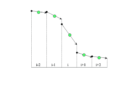
Figure 9: Same as Figure 8, but using the monotonic-centered reconstruction. Notice that the interface values are bounded now between the neighbor nodes, so that monotonicity is preserved both for the left values (arrows) and for the right ones (dots) at every interface (dotted lines).

We can see in Fig. 8 an example of the reconstruction process for the centered choice

$$\Delta^{C}_{i}=\frac{1}{2}~{}(F_{i+1}-F_{i-1})\,.$$ (II.6)

The outcome consists in two sequences of one-sided predictions at every interface (dots and arrows). Notice that the monotonicity of the original Flux sequence is not preserved by the one-sided predictions in the regions with abrupt slope changes. This can lead to spurious oscillations in the numerical solution, even for smooth dynamical fields, like the one displayed in Fig. 8. These spurious oscillations are visible in the Black Hole simulation shown in Fig. 2.

The MMC method uses instead a monotonicity-preserving prescription, which can be obtained by using the ’monotonic centered’ (MC) slope vanLeer77

$$\Delta^{MC}_{i}\equiv minmod\{\,2(F_{i}-F_{i-1}),\,2(F_{i+1}-F_{i}),\,\Delta^{C}_{i}\}$$ (II.7)

instead of (II.6). The $minmod$ function is defined as usual:

• If all the arguments have the same sign, then it selects the one with smaller absolute value.

• If one of the arguments has different sign than the others, then it is zero.

In this way, the slopes are limited in order to avoid spurious oscillations. The rule is that interface values must lie between their neighbor node values (see Figure 9).

The second ingredient in the MMC method is the use of Marquina’s Flux formula Marquina . The prescription to calculate the interface values $\mathbf{F}_{i+1/2}$ can be stated as follows (we have simplified the original formula by adapting it to the quasilinear evolution systems one gets from Einstein’s field equations):

• Decompose both one-sided predictions $(\mathbf{F}^{L}\,,~{}\mathbf{F}^{R})$ as linear combinations of the set of characteristic fields $\mathbf{w}$. Note that the coefficients in these combinations are not necessarily constant: we must use in general a different set of values on each side of the interface.

• Project the forward prediction $\mathbf{F}^{L}$, by suppressing any components $\mathbf{w}$ corresponding to negative characteristic speeds (forward projection $\mathbf{F}_{F}$).

• Project the backward prediction $\mathbf{F}^{R}$, by suppressing any components $\mathbf{w}$ corresponding to positive characteristic speeds (backward projection $\mathbf{F}_{B}$).

• Add these upwind-projected values at the given interface, that is

  $$\mathbf{F}_{i+1/2}~{}=~{}\mathbf{F}_{F}+\mathbf{F}_{B}\,.$$ (II.8)

One is taking in this way the positive speed components from the previous cell and the negative speed components from the next one. Notice that we must assume for consistency a definite sign for the characteristic speed (just the sign, not even the value). If the sign changes between both sides of the given interface (when using a super-luminal shift, for instance), then another combination must be taken instead of the simple upwind projections presented here (see Ref. Marquina for the details).

Acknowledgements: This work has been supported by the EU Programme ’Improving the Human Research Potential and the Socio-Economic Knowledge Base’ (Research Training Network Contract HPRN-CT-2000-00137), by the Spanish Ministerio de Ciencia y Tecnologia through the research grant number BFM2001-0988 and by a grant from the Conselleria d’Innovacio i Energia of the Govern de les Illes Balears.

References

- (1) R. Arnowit, S. Deser and C. W. Misner. In: Gravitation: an introduction to current research, ed. by L. Witten, Wiley, (New York 1962).
- (2) L. Smarr and J. W. York, Phys. Rev. D17, 1945 (1978), Phys. Rev. D17, 2529 (1978).
- (3) F. Estabrook et al., Phys. Rev. D7, 2814 (1973).
- (4) B. Reimann, gr-qc/0404118, (2004).
- (5) C. Bona, J. Massó, E. Seidel and J. Stela, Phys. Rev. Lett. 75 600 (1995).
- (6) Y. Choquet-Bruhat and T. Ruggeri, Comm. Math. Phys. 89, 269 (1983).
- (7) C. Bona and J. Massó, Phys. Rev. D38, 2419 (1988).
- (8) P. Anninos et al, Phys. Rev. D52 2059 (1995).
- (9) M. Alcubierre, Phys. Rev. D55, 5981 (1997).
- (10) M. Alcubierre, Class. Quantum Grav. 20, 607 (2003).
- (11) M. Shibata and T. Nakamura, Phys. Rev. D52 5428 (1995).
- (12) T. W. Baumgarte and S. L. Shapiro, Phys. Rev. D59 024007 (1999).
- (13) D. Pollney, private communication.
- (14) C. Bona, T. Ledvinka, C. Palenzuela, M. Žáček, Phys. Rev. D67 104005 (2003).
- (15) C. Bona, T. Ledvinka, C. Palenzuela, M. Žáček, Phys. Rev. D69 064036 (2004).
- (16) B. van Leer, J. Comput. Phys. 23, 276 (1977).
- (17) R. Donat and A. Marquina, J. Comp. Phys. 125, 42 (1996).
- (18) S. L. Shapiro and S. A. Teukolsky, In: Dynamical Spacetimes and Numerical Relativity, ed. by J. M. Centrella, Cambridge University Press, (Cambridge, UK 1986).
- (19) P. Anninos et al, Phys. Rev. D51 5562 (1995).
- (20) B. Reimann and B. Brügmann, Phys. Rev. D69 044006 (2004).
- (21) H.O. Kreiss and J. Lorentz, Initial-Boundary problems and the Navier-Stokes equations, Academic Press, New York (1989).
- (22) O. A. Liskovets, Differential equations I 1308-1323 (1965).