Chen-Wu type model and the total energy of the universe

Abstract

The inclusion of a $\Lambda$ term, today, in the relativistic field equations is consequence of the evolution of an observational cosmology. In this work we argue the "ansatz" $\Lambda=\beta H^{2}+\frac{\alpha}{R^{2}}$ is applicable to the total energy density of the universe, discuss some cosmological consequences and compare the growing mode of the density contrast with the corresponding mode of the standard model.

1 Introduction

The cosmological scale factor obtained integrating the Einstein field equations , considering the universe as homogeneous and isotropic, has been subject of study in a numerous quantity of works. Generally, textbooks given more attention to the models with null pressure and absence of a cosmological constant or term.

Sir A. Eddington looked for meaning of the $\Lambda$ term in the Einstein field equations. He declare that $\Lambda$ term corresponds to the absolute energy in a standard zero condition. Eddington seems to believe in the necessity of $\Lambda$ as zero point, although he do not explain why not consider $\Lambda=0$, of fact. Eddington wrote later: “ $\Lambda$ can not be zero because the zero condition must correspond to a possible rearrangement of the matter of the universe” [1]. Otherwise, George Lemaitre considered that the conventional level used to count energy, taking into account $\Lambda=0$, can not be set as fundamental.

In spite of the arguments to preserve the cosmological term, de Sitter and Einstein joint to a group that has a opinion in favor of its rejection, in spite of Einstein himself was one of the pioneer of the inclusion of $\Lambda$ in the relativistic field equations of gravitation. Moreover, in light of the experimental evidence of the expansion of the universe, Einstein considered the inclusion of $\Lambda$ as “ the biggest blunder of my life” [2].

In the present time, the cosmological science indicates that we must have a non-zero cosmological term. Krauss and Turner [3] in your work look the return of the cosmological constant. They cited the age of the universe, the formation of the large scale structure and the matter content of the universe as the data that cry out by a cosmological constant. In another hand, the data obtained from the observations of the supernova of type IA, by two independent teams [4], [5], indicates that the universe has an accelerated expansion.

New problems appear with the inclusion of $\Lambda$ as a constant. Some of them are old today, as the problem about the discrepancy (50 - 120 orders of magnitude) among the observed value for the present energy density of the vacuum and the large value suggested by the particle physics standard model [6]. An alternative to avoid this problem is assume that the effective cosmological term evolves and decreases to its present value. So, when we refer to $\Lambda$ as a cosmological term, we consider that $\Lambda$ is a time-dependent function.

The inclusion of $\Lambda$ term in the field equations is one of the possibilities to generate a negative pressure content in the universe, responsible by the cosmic acceleration.

W. Chen and Y. Wu [7] study a cosmological model with a cosmological term given by $\Lambda\propto R^{-2}$ using a dimensional argument based in conformity with quantum cosmology. The authors claim that the “ ansatz” adopted for $\Lambda$ is not in conflict with the observational data and can alleviate some problems in relation to the inflationary scenario. Some years after, Carvalho and Lima extended the work of Chen and Wu, including $\Lambda=\beta H^{2}+\alpha R^{-2}$. The authors look that the Chen and Wu model do not comprise a negative value for deceleration parameter ( $q$ ) today, but alleviates the density parameter problem. Otherwise, Carvalho and Lima [8] model furnishes $q<0$ and the agreement with nucleosynthesis predictions can be put in terms of the phenomenological parameters of the model. Relaxing the hypothesis that the phenomenological constants of the model have the same values during the radiation and matter eras, it is easy to satisfy the nucleosynthesis constraints.

Posteriorly, John and Joseph [9] argue that the Chen-Wu “ansatz” can be applicable to the total energy density of the universe, in place of the vacuum density alone. Since that the Planck era is characterized by the Planck density , the Chen-Wu “ ansatz” is better adequate when applied to the total energy density. The resulting model, according the authors, is free of the horizon, flatness, monopole, generation of density perturbations problems.

Our intent in this work is extended the Jonh and Joseph work in a similar sense that Carvalho and Lima extended the Chen and Wu work. We also discuss the growing modes for density contrast and compare its evolution with the growing mode of the standard model.

2 The Model

Let us consider the universe as homogeneous and isotropic, described by the line element

$$ds^{2}=dt^{2}-R(t)^{2}[\frac{dr^{2}}{1-\kappa r^{2}}+r^{2}(d\theta^{2}+sin^{2}(\theta)d\phi^{2})]\,,$$ (1)

where $\kappa$ is the curvature parameter.

Describing the universe as a comoving perfect fluid with a $\Lambda$ term, the Einstein field equations assumes the form

$$3H^{2}+\frac{3\kappa}{R^{2}} = 8\pi G(\rho_{m}+\rho_{\Lambda})\,,$$ (2)

$$2\frac{\ddot{R}}{R}+\frac{\dot{R}^{2}}{R^{2}}+\frac{\kappa}{R^{2}} = -8\pi G(P-\rho_{\Lambda})\,,$$ (3)

where $\rho_{m}$, $\rho_{\Lambda}$ and $P$ are, respectively, the matter energy density, the $\Lambda$ energy density and the pressure.

Extended the Chen-Wu argument to the total density of the universe, we can write

$$\rho_{m}+\rho_{\Lambda}/3=\xi\,,$$ (4)

where $\xi$ is a time dependent function and the $\frac{1}{3}$ in (4) is included for mathematical convenience. With help of equations (2) (3) and (4) we can write the field equation

$$4\frac{\ddot{R}}{R}-(7+3\nu)(H^{2}+\frac{\kappa}{R^{2}})+24\pi G(1+\nu)\xi=0\,.$$ (5)

The constant $\nu$ in equation (5) is defined by the state equation $P=\nu\rho$.

Taking into account the “ansatz”, used by Carvalho et. al [8] to the total energy density of the universe the function $\xi$ assumes the form

$$\xi=\frac{1}{8\pi G}\{\beta H^{2}+\frac{\alpha}{R^{2}}\}\,.$$ (6)

Therefore, eq. (5) can be written as

$$R\ddot{R}+\alpha_{1}\dot{R}^{2}+K_{1}=0\,,$$ (7)

where $\alpha_{1}=-1+\frac{3(1+\nu)(\beta-1)}{4}$ and $K_{1}=-\kappa+\frac{3(1+\nu)(\alpha-\kappa)}{4}$.

Integrating equation (7), the solution can be put in the form

$$\pm R^{\alpha_{1}+1}\frac{{}_{2}F_{1}\{[\frac{1}{2},\frac{\alpha_{1}+1}{2\alpha_{1}}],[\frac{3\alpha_{1}+1}{2\alpha_{1}}],\frac{R^{2\alpha_{1}}K_{1}}{a}\}}{2(a\alpha_{1})^{1/2}[\frac{\alpha_{1}+1}{2\alpha_{1}}]}=t+b\,,$$ (8)

where ${}_{2}F_{1}$ denotes a hypergeometric function and the integration constants are denoted by $a$ and $b$.

The contents of the universe can be considered in the field equations using the density parameters

$$\Omega_{\Lambda} \equiv \frac{\rho_{\Lambda}}{\rho_{c}}$$

$$\Omega_{m} \equiv \frac{\rho_{m}}{\rho_{c}}\,,$$

for $\Lambda$ and matter contents, respectively. The $\rho_{c}$ is the critical density and is given by $\rho_{c}=\frac{3H^{2}}{8\pi G}$.

Considering the universe flat and using the field equations (2) and (3) we find

$$\Omega_{\Lambda} = \frac{1}{2}\{3-\beta-\frac{\alpha}{\dot{R}^{2}}\}$$ (9)

$$\Omega_{m} = \frac{1}{2}\{-1+\beta+\frac{\alpha}{\dot{R}^{2}}\}\,.$$ (10)

We can write eqs. (9) and (10) in the form

$$\dot{R}^{2}=\frac{2+(1+\gamma)(1-\beta)}{\alpha(1+\gamma)}\,,$$ (11)

where

$$\gamma=\frac{\Omega_{\Lambda}}{\Omega_{m}}\,.$$ (12)

Naturally $\gamma$ depends of the cosmological era.

Rewritten the field equation (7) as

$$q=\alpha_{1}+\frac{K_{1}}{\dot{R}^{2}}$$ (13)

and using expression (11) we find an expression among the deceleration parameter ($q$) and the fenomenological parameters of the model, namely

$$q=-\frac{7-3\beta}{4}+\frac{3\alpha^{2}}{4[1-\beta+\frac{2}{1+\gamma}]}\,.$$ (14)

Although, the expression (14) is interesting from the observational point of view and we obtain it without an explicit expression for the scale factor, an explicit form for $R(t)$ is useful for study the age and creation of small inhomogeneities in the universe.

With a adequate choose of the parameters we can write the expression (8) for the scale factor in a more suitable form. We guide our choose using equation (13). Note that assuming $K_{1}=0\longrightarrow q=\alpha_{1}$. So, taking into account $K_{1}$ null we obtain a potential solution for the scale factor.

$$R(t)=[(1+\alpha_{1})t]^{\frac{1}{1+\alpha_{1}}}\,.$$ (15)

Consequently the Hubble function and the deceleration parameter are given, respectively by

$$H=\frac{4}{3(1+\nu)(\beta-1)t}$$ (16)

and

$$q=-1+\frac{3(1+\nu)(\beta-1)}{4}.$$ (17)

Note that, the universe has an accelerated expansion if $1<\beta<\frac{7}{3}$. However, for $\nu=0$ the Hubble function $H=\frac{4}{3(\beta-1)t}$ results in a universe older than the established by the standard model if $\beta<3$. So, taking into account the accelerated expansion of the universe, in accord with the observations from supernova IA, and the age of the oldest objects in our galaxy that estimates an inferior limit for the age of the universe, in contradiction with the predictions of the standard model [10] ,we can infer a validity range for $\beta$, $1<\beta<\frac{7}{3}$.

For $K_{1}=0\longrightarrow\alpha=\frac{7\kappa}{3}$, so for different values for the curvature parameter $\kappa$ the evolution of the scale factor (15) is not sensible to the $\kappa$ value. In other hand, for different values for $\beta$ the scale factor evolve differently as show in the Fig.1.

Figure 1: Evolution of the scale factor (15) for $\beta=1.5$ and $\beta=2.5$ and the scale factor of standard model, signed with $\&$.

We obtain a coasting type solution [11] if $\alpha_{1}=K_{1}=0$ and for $\beta=3$ we obtain a scale factor that mimics the standard model, although the barionic density differs in the two models.

In other hand, a type de Sitter solution can be obtained substituting $\beta=1$ in (7), obtaining

$$R(t)=\frac{a}{2}\{\frac{1}{\exp{\frac{t+b}{\pm a}}}-K1\exp{\frac{t+b}{\pm a}}\}\,,$$ (18)

where the profile is given in the Fig.2

Figure 2: Evolution of the scale factor (18) for $\beta=1$ and $\alpha=-1$.

3 Scalar perturbations

Although the universe is considered homogeneous at large scales, we have inhomogeneities at small scales. These inhomogeneities are originated from small scalar perturbations in the homogeneous background.

The Newtonian formalism is not adequate to study large scale perturbations without invoke procedures which are mathematically dubious [12]. Although, in regions much smaller than the characteristic length scale, the Newtonian cosmology can be used as an approximation to general relativity and in such regions there exists a natural choice of coordinates in which Newtonian gravity is applicable. So, we study the formation of the inhomogeneities in the universe using scalar perturbations in the relativistic framework.

The relativistic equation,in a universe without $\Lambda$, for the density contrast is given by [12]:

$$\ddot{\delta}(t)+[2-3(2\nu-v^{2})]H\dot{\delta}(t)-\frac{3}{2}H^{2}\delta(t)(1-6v^{2}-3\nu^{2}+8\nu)=-(\frac{kv}{a})^{2}\,,$$ (19)

where $\delta$ is the density contrast defined by $\delta=\frac{\delta\rho}{\rho}$ and $\delta\rho$ is the density perturbation. Considering $\nu=0$ and $v\sim 0$ and using the field equation for a universe without a cosmological term $H^{2}=\frac{8\pi G\rho}{3}$ we obtain

$$\ddot{\delta}(t)+2H\dot{\delta}(t)-4\pi G\rho\delta(t)=0$$ (20)

So, under the circumstances described above the relativistic equation for $\delta$ decay in the analogue Newtonian equation.

We can obtain the equation for the density contrast in a universe with a cosmological term in a non canonical, but correct method. Substituting equation (2) in the equation (20) we obtain

$$\ddot{\delta}(t)+2H\dot{\delta}(t)-\frac{3}{2}H^{2}\delta(t)+\frac{1}{2}\Lambda\delta(t)=0$$ (21)

The integration of equation for the density contrast using the scale factor (21) furnishes the modes

$$\delta(t)_{\pm}=t^{\frac{-11+3\beta\pm\sqrt{73-18\beta+9\beta^{2}}}{6\beta-6}}\,.$$ (22)

To have an idea about the evolution of the density contrast in this model compared with the standard model we define the quantity

$$f:={\delta_{c}(t)}-{\delta_{s}(t_{d})}\,,$$ (23)

where the sub-script $s$ and $c$ refers to the standard and Chen-Wu models, respectively. The profile of $f$ is given in the Figure 3.

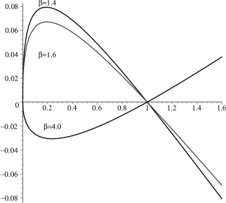
Figure 3: $f\times t$ for several values of $\beta$.

Note that at early times the mode $\delta_{c+}$ grows faster than the respective mode for the standard model. So, in our model we can say that the inhomogeneities are formed more easily and the non linear regime is reached before than the standard model.

In other hand, using the scale factor (18) and integrating the equation for the density contrast the modes obtained are:

$$\delta_{a}(t) \propto {{}_{2}F_{1}}\{[\frac{1}{2}+a,\frac{3}{2}+a],[1+2a],-K_{1}e^{2t}+1\}e^{2t}(-1+K_{1}e^{2t})^{a-\frac{1}{2}}\,,$$ (24)

$$\delta_{b}(t) \propto {{}_{2}F_{1}}\{[\frac{3}{2}-a,\frac{1}{2}-a],[1-2a],-K_{1}e^{2t}+1\}e^{2t}$$

$$(1-K_{1}e^{2t})^{-2a}(K_{1}e^{2t}-1)^{a-\frac{1}{2}}\,,$$

where $a=\frac{\sqrt{(K_{1}-3)K_{1}}}{2K_{1}}$. The profile of the density contrast (24) for $K_{1}=-\frac{3}{8}$ is given in the Fig.(4).

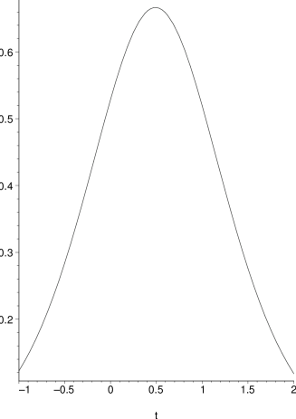
Figure 4: Evolution for (24) with $K_{1}=-\frac{3}{8}$.

For early times the density contrast (24) grows faster than the standard model. Note that the density contrast (24) grows with a posterior decaying, corresponding to the contracting and expansion of the universe governed by the scale factor (18). For early times the density contrast (24) grows faster than the standard model, as can conclude look the profile for $f$ in Fig.5.

Figure 5: $f\times t$

4 Conclusions

In this work we generalized the work of Carvalho and Lima in the same sense that Jonh and Joseph generalized the work of Chen and Wu, previously cited. Our model do not create conflicts with the observational evidence with respect to the acceleration and age of the universe and the fenomenological constants of the model can be adjust to the nucleosynthesis predictions.

Our model of the universe is accelerated and we find the analytical expressions for the growing modes for the density contrast and compare with evolution of the growing mode for the standard model.

References

- [1] North, J. D., The Measure of the Universe. Dover Publications, New York, (1965).
- [2] Gamov, G., My World Line. Viking, New York, (1970).
- [3] Krauss, L. M. and Turner, M., Gen. Relat. Grav., 27, 1137, (1995).
- [4] Perlmutter, S., et al., Astrophys. J., 517, 565, (1999).
- [5] Riess, A., et al., Astrophys. J., 116, 1009, (1998).
- [6] Weinberg, S., Rev. Mod. Phys., 61, 1, (1989).
- [7] Chen, W. and Wu, Y., Phy. Rev. D, 41, 695, (1990).
- [8] Carvalho, J. C. and Lima. J. A. S., Phy. Rev. D, 46, 2404, (1992).
- [9] John, M and Joseph, K., Phy. Rev D, 61, 087304, (2000).
- [10] Krauss, L. M., Phy. Rep, Volume 333-334, 33-45, (2000).
- [11] Kolb, Edward W., Astrophys. J., Volume 344, 543-549, (1989).
- [12] Padmanabhan, T., Structure formation in the universe. Cambridge University Press, Cambridge, (1993).