Self-consistent invariant dynamics of scalar perturbations in the inflationary cosmology

Abstract

The gauge-independent invariant approach to investigation of the linear scalar perturbations of inflaton and gravitational fields is developed in self-consistent way. This approach allows to compare various gauges used by other researchers and to find unambiguous selection criteria of physical and coordinate effects. We have shown that the so-called longitudinal gauge commonly used for studying the gravitational instability leads to overestimation of physical effects due to the presence of nonphysical proper time perturbations. Equation of invariant dynamics (EID) is derived. The general long-wave solution of EID for an arbitrary potential $U(\phi)$ has been obtained. We have also found analytical solutions for all wave lengths at all stages of the universe evolution in the framework of simplest potential $U(\varphi)=m^{2}\varphi^{2}/2$. We have constructed the analytical expressions for the energy density perturbations spectrum $\Delta(k,t)$ at all possible $k$ and $t$. Amplitude of the long-wave spectrum in the case of the transition from short waves to long ones occurs at the inflationary stage is almost flat, i.e. has the Harrison-Zeldovich form, for arbitrary potential $U(\varphi).$

I Introduction

The standard inflationary model Guth ; Linde0 ; Linde1 is the most successful theoretical model for explanation of the observable Universe structure. According to this model at the early stages the Universe was in an unstable vacuum-like state characterized by a slow linear drop of the Hubble parameter $H(t)$ with time growth thus the cosmological expansion had a quasiexponential character

$$a(t)\sim\exp\int\limits_{0}^{t}H(t)dt.$$

This stage of evolution of the Universe is called the inflationary epoch. For reviews on inflationary cosmology see Refs. Linde2 ; Albrecht ; Lazarides .

The simplest model of the cosmological inflation for the flat universe is described by Lagrangian

$${\cal L}=-\frac{1}{2\varkappa}\hat{R}(\hat{g}_{ik}) + \frac{1}{2}\hat{g}^{ik}\hat{\varphi}_{,\;k}\hat{\varphi}_{,\;i}-U(\hat{\varphi}).$$ (1)

Einstein equations for this model are

$$\hat{R}_{i}^{k}-\frac{1}{2}\delta_{i}^{k}\hat{R}=\varkappa\hat{T}_{i}^{k},\qquad\hat{T}_{i}^{k} = \hat{\varphi}_{;i}\hat{\varphi}^{;k}-\delta_{i}^{k}\left(\frac{1}{2}\hat{\varphi}_{;l}\hat{\varphi}^{;l}-U(\hat{\varphi})\right),$$ (2)

where $\varkappa=1/M_{Pl}^{2}$ is the gravitational constant, $M_{Pl}$ is the Plank mass. The equation of motion of the inflaton field is

$$\hat{\varphi}_{;i}^{;i}+\frac{\partial U(\hat{\varphi})}{\partial\hat{\varphi}} = 0.$$ (3)

The symbol “^” here implies that metric $\hat{g}_{ik}$ and inflaton (scalar) field $\hat{\varphi}$ are quantum operators. We will divide their into the classical spatially homogeneous parts denoted $g_{ik}$ and $\varphi(t)$ correspondingly and the quantum fluctuation operators $\chi(t,\vec{x})$ and $h_{ik}(t,\vec{x})$, describing small perturbations.

The main properties of the inflationary universe may be seen in the model with quadratic potential Linde0

$$U(\hat{\varphi})=\frac{1}{2}m^{2}\hat{\varphi}^{2}.$$ (4)

This model is used in our work for describing of some new aspects of the self-consistent invariant dynamics of inflaton and gravitational fields.

Traditionally there are three main problems in the framework of the model (1). The first problem is concerned with the self-consistent dynamics of spatially homogeneous fields

$$\varphi(t)=\langle\hat{\varphi}\rangle,\qquad g_{ik}=\langle\hat{g}_{ik}\rangle=diag(1,\;-a^{2}(t),\;-a^{2}(t),\;-a^{2}(t)).$$

that is described by equations (2) and (3) in the zeroth order of perturbation theory:

$$\begin{array}[]{l}\displaystyle 3H^{2}=\varkappa\left(\frac{1}{2}\dot{\varphi}^{2}+U(\varphi)\right),\\[14.22636pt] \displaystyle\ddot{\varphi}+3H\dot{\varphi}+\frac{\partial U(\varphi)}{\partial\varphi}=0.\end{array}$$ (7)

Here $H=\dot{a}/a$. In further calculations we’ll use both the cosmic time $t$ ($g_{00}=1$) and the conformal time $\eta$ ($g_{00}=a^{2}$). Recall, the dot “ $\dot{}$ ” denotes a derivative with respect to the cosmic time, the prime “ ^′ ” denotes one with respect to the conformal time.

Solution of this problem is well-known and underlies the chaotic inflation scenario Linde0 . We have unified the corresponding calculations. The system of background equations (7) is solved analytically at all times $t$. Consideration of dynamical properties for the simplest inflation model is necessary for solution of the second problem:

The second problem is connected with the self-consistent dynamics of spatially inhomogeneous quantum fluctuations of inflaton and gravitational fields

$$\chi(t,\vec{x})=\hat{\varphi}(t,\vec{x})-\varphi(t),\qquad h_{ik}(t,\vec{x})=\hat{g}_{ik}(t,\vec{x})-\langle\hat{g}_{ik}\rangle$$

both at inflationary and postinflationary stages of the Universe evolution. The theory of cosmological perturbations is based on expanding the Einstein equations to linear order about the background metric. The theory was initially developed in pioneering works by Lifshitz Lifshitz . Two aspects of the problem are: (i) the stability of the inflationary process; (ii) the back reaction of the long-length perturbations on the expansion of the Universe in the past and in the present epoch Abramo .

The third problem is how the Harrison-Zeldovich spectrum HarZel was formed from the inflaton field vacuum fluctuations, the length of which is much less than the Universe size at the beginning of the inflation. As it is known, the solution of this problem is the basis for the modern theory of the large scale structure formation in the Universe.

A large amount of papers is devoted to solving the last two problems mentioned above which has been investigated by various researches for more than twenty years. The conventional approach is based on the investigation of the scalar perturbations in the so-called diagonal or longitudinal gauge as the most comfortable. The theory is formulated in terms of the relativistic scalar potential $\Phi(\vec{x},t)=\delta g_{00}(\vec{x},t)$; all other observable values are expressed via $\Phi(\vec{x},t)$. The subject of the discussion, which constantly appears in the literature, is if the predictions of the physical consequences of the theory are invariant. Two point of view clashed at this point. Some people suppose, that the longitudinal gauge is physically preferred because its main object, $\Phi(\vec{x},t)$, is invariant itself Mukh . The opposite claim is that $\Phi(\vec{x},t)$ describes effects in the fixed frame of reference Unruh ; Grisch ; in other frames of reference the observed phenomena may look in another way.

In fact, the question is if the theory in the longitudinal gauge can be used to reconstruct the past of the Universe on the basis of the observations that will be performed. The Fourier-image of $\Phi_{{\bf k}}(t)$ is the functional $\Phi_{{\bf k}}\{H(t)\}$, and the Hubble function $H(t)$ contains information about the inflaton field and the inflationary process itself. The theoretical reconstruction of the past is possible only in the case of $\Phi_{{\bf k}}\{H(t)\}$ is an invariant functional. On the other hand, in the case of the information contained in $\Phi_{{\bf k}}\{H(t)\}$ essentially depends on the properties of the frame of reference that is prescribed by the longitudinal gauge, the theory of relativistic scalar potential can not be used to interpret the results of the experiment.

Our claim — that the theory in the longitudinal gauge is noninvariant — is made on the basis of the proposed invariant dynamics of the scalar perturbations. The main result of our investigation is the strict proof of the following statement. The invariant information about the dynamics of the scalar perturbations is selected from the equations of the linear gravitational instability theory by the identical mathematical transformations without making use of any gauge condition at any stage of the calculations. Our theory is formulated as a closed system of equations for the invariant $J_{\bf k}$ of metric perturbations, invariant function $\chi_{{\bf k}{\rm inv}}$ of the perturbations of the inflanton field, its derivative $\dot{\chi}_{{\bf k}{\rm inv}}$ and energy density perturbations $\delta\varepsilon_{\rm inv}.$ The theory is such that the invariance of the physical values follows from their mathematical definitions, and the invariance of the equations does from the way to obtain them without any gauge.

Invariant approach allows us to compare different gauges which are used in the works of other researches and to find unambiguous separation criteria of physical and coordinate effects. The problem of such criteria existence was widely discussed also in Linde1 ; Mukh ; Unruh ; Grisch . We have shown that the longitudinal gauge leads to the overestimation of the physical effect as a result of the strong perturbations of the proper time in frame of reference specified by the longitudinal gauge. The general qualitative properties — the power-law instability of long-length perturbations and the formation of the Harrison-Zeldovich spectrum — are the same in the two approaches, but the numerical values are different, the perturbations in the longitudinal gauge theory being several times greater. Invariant approach excludes nonphysical coordinate effects and gives a key for analytical investigation of equations in the perturbation theory that is the aim of our work.

Among the theories formulated in the fixed gauges, the synchronous gauge theory proposed by Lifshitz Lifshitz is an adequate one, because it this gauge the evolution of the background and perturbations is analyzed in one and the same time.

We have analytically investigated of the equation of invariant dynamics (EID) for $J_{\bf k}.$ The general long-wave solution of EID as a functional of background solution for arbitrary potential $U(\phi)$ is obtained. For one of the simplest model of inflaton field (4) we have found explicit solutions of EID for all wave numbers $k$ and times $t$. An important point of our investigation is that both the background characteristics and characteristics of perturbations at the inflationary and postinflationary stages in the considering model (1) of the Universe are completely defined by the parameter $m$ and the initial values of the Hubble function $H_{0}$ and the scale factor $\tilde{a}_{0}.$

II Background dynamics: an analytical glance at the Linde’s chaotic inflation

The system (7) for potential (4) turns to

$$\begin{array}[]{l}\displaystyle\dot{H}=-\frac{\varkappa}{2}\dot{\varphi}^{2},\\[14.22636pt] \displaystyle\ddot{\varphi}+3H\dot{\varphi}+m^{2}\varphi=0.\end{array}$$ (10)

In the limit $t\to 0$ solutions of this system can be represented as power series

$$\varphi(t)=\sum_{n=0}^{\infty}a_{n}t^{n},\qquad H(t)=\sum_{n=0}^{\infty}b_{n}t^{n}.$$ (11)

Substituting (11) in the (10) we obtain the system of equations

$$\begin{array}[]{l}\displaystyle\sum_{n=0}^{\infty}nb_{n}t^{n-1}=-\frac{\varkappa}{2}\sum_{k,n=0}^{\infty}kna_{k}a_{n}t^{k+n-2},\\[14.22636pt] \displaystyle\sum_{n=0}^{\infty}n(n-1)a_{n}t^{n-2}+3\sum_{k,n=0}^{\infty}na_{n}b_{k}t^{k+n-1}+m^{2}\sum_{n=0}^{\infty}a_{n}t^{n}=0.\end{array}$$ (14)

The initial value of $H(t)$ unambiguously defines the initial values of functions $\varphi(t)$ and $\dot{\varphi}(t)$. For convergence of series we should assume that

$$\frac{m^{2}}{9\,b_{0}^{2}}\ll 1,\qquad m\ll 1,\qquad a_{2}=0.$$ (15)

Taking into account these conditions we will receive from (14) the following relations for $a_{n}$ and $b_{n}$:

$$\begin{array}[]{l}\displaystyle a_{0}=\frac{b_{0}}{m}\left(\frac{6}{\varkappa}\right)^{1/2},\;a_{1}=-\frac{m}{3}\left(\frac{6}{\varkappa}\right)^{1/2},\;a_{3}=\frac{m^{5}}{162\,b_{0}^{2}}\left(\frac{6}{\varkappa}\right)^{1/2},\;a_{n}=-\frac{3}{n}\,b_{0}a_{n-1}\quad\mathrm{for}\quad n\geqslant 4;\\[14.22636pt] \displaystyle b_{1}=-\frac{\,m^{2}}{3},\qquad b_{2}=0,\qquad b_{n}=-\varkappa{a_{1}}{a_{n}}\quad\mathrm{for}\quad n\geqslant 3.\end{array}$$

Therefore the expression for expansion coefficient of function $H(t)$ is

$$b_{n}=(-1)^{n+1}\>\frac{6m^{6}}{81b_{0}^{2}}\>\frac{(3b_{0})^{n-3}}{n!}.$$

The series can be summed up and the result is

$$H(t)=b_{0}-\frac{\,m^{2}}{3}\>t+\frac{m^{6}t^{2}}{81b_{0}^{3}}-\frac{2m^{6}}{729b_{0}^{5}}\left(e^{-3b_{0}t}-1+3b_{0}t\right).$$ (16)

For small $t$ due to conditions (15) this expansion corresponds to the linear approximation – peculiar feature of the inflationary epoch (Fig. 1):

$$H(t)=H_{0}-\frac{\,m^{2}}{3}\>t.$$ (17)

Let us build an analytical solution of (10) in the limit $t\rightarrow\infty,$ corresponding to the postinflationary stage. As it is known in this limit the Hubble function $H(t)$ must approach to $2/{3t}$ of present-day Friedman’s universe. In the equation $\ddot{\varphi}+3H\dot{\varphi}+m^{2}\varphi=0$ one can make the substitution $\varphi=\psi/a^{3/2}$. As a result we have

$$\ddot{\psi}+\psi\left(m^{2}-\frac{3}{2}\,\dot{H}-\frac{9}{4}\,H^{2}\right)=0.$$ (18)

This is the equation of oscillator with the variable frequency $\omega(t)^{2}=m^{2}+\rho(t)$, where $\rho(t)=-\frac{3}{2}\,\dot{H}-\frac{9}{4}\,H^{2}\rightarrow 0$ steadily for $t\rightarrow\infty$. The general solution of equations like (18) has the form:

$$\psi(t)=\frac{C_{1}}{\sqrt{2\varepsilon(t)}}\>e^{-i\int_{a}^{t}\varepsilon(t)dt}+\frac{C_{2}}{\sqrt{2\varepsilon(t)}}\>e^{i\int_{a}^{t}\varepsilon(t)dt},\quad C_{2}=C_{1}^{*}.$$ (19)

The function $\varepsilon(t)$ should be defined. Substituting (19) in (18) and differentiating we obtain:

$$\frac{d}{dt}(m^{2}+\hat{I})D=0,$$ (20)

where $D(t)=1/\varepsilon(t)$, $\hat{I}$ is the integro-differential operator, which is defined as

$$\hat{I}f=\frac{1}{4}\left(\frac{d^{2}}{dt^{2}}f+2\rho{f}+2\int_{\infty}^{t}dt\rho\frac{d}{dt}f\right),$$

for example, $\hat{I}\,1=\rho/2$, $\hat{I}\rho=\frac{1}{4}(\ddot{\rho}+3\rho^{2}).$ Equation (20) gives

$$D(t)=\frac{const}{m^{2}\left(1+\frac{\hat{I}}{m^{2}}\right)}=\frac{1}{m}\sum_{n=0}^{\infty}(-1)^{n}\left(\frac{\hat{I}}{m^{2}}\right)^{n}.$$

Constant has been chosen for correspondence to zeroth approximation of equation (18) – the harmonic oscillator with the frequency $m$. Suffice it to take into account just a first correction. Finally we have

$$\varepsilon=m\left(1-\frac{1}{8m^{2}}(6\dot{H}+9H^{2})\right).$$ (21)

Then instead of $\varphi$ we introduce the new function $G=\psi^{2}$, as a result we get

$$3H^{2}=\frac{\varkappa}{a^{3}}\left(\frac{1}{4}\ddot{G}+m^{2}G-\frac{3}{4}(HG)\dot{}\right).$$ (22)

On the other hand using (19) and (21) we have up to the first order terms of $1/t$ inclusively

$$G\equiv\psi^{2}=\frac{1}{m}\left(1+\cos(2mt+\alpha)+\left(\frac{3H}{2m}+\frac{9}{4m}\int_{a}^{t}H^{2}{dt}\right)\sin(2mt+\alpha)\right).$$ (23)

Substituting this expression in (22) we get an equation for $H(t)$:

$$3H^{2}=\frac{\varkappa}{a^{3}}\left(m+\frac{3H}{2}\sin(2mt+\alpha)\right).$$

This equation has been solved by substitution $a(t)=e^{\int H(t)dt}$ then by taking the logarithm and differentiation. Up to the second order terms of $1/t$ inclusively we get the following asymptotic solution of the system (10) for $t\rightarrow\infty$:

$$H(t)=\frac{2}{3(t-t_{0})}+\frac{1}{3m(t-t_{0})^{2}}\sin(2m(t-t_{0})+\alpha).$$ (24)

This solution corresponds to the postinflationary stage of the Universe (Fig. 1). Two parameters — shift parameter $t_{0}$ and initial phase $\alpha$ — can be found by matching of background solutions (17) and (24).

Figure 1: Hubble function as a function of cosmic time at the inflationary (left) and postinflationary (right) stages; $H_{0}=1$, $m=0.15$ (system of units $\hbar=c=8\pi G=1$), $t_{1}\simeq 127$, $t_{0}\simeq 113$.

Let $t_{1}$ is the transition time of the Universe from inflationary to postinflationary stage. At $t=t_{1}$ we require an execution of the following three conditions:

1. Continuity condition of $H(t)$:

   $$H_{0}-\frac{\,m^{2}}{3}\>t_{1}=\frac{2}{3(t_{1}-t_{0})}+\frac{1}{3m(t_{1}-t_{0})^{2}}\sin(2m(t_{1}-t_{0})+\alpha);$$

2. Smoothness condition of $H(t)$:

   $$-\frac{\,m^{2}}{3}=-\frac{2}{3(t_{1}-t_{0})^{2}}+\frac{2}{3(t_{1}-t_{0})^{2}}\cos(2m(t_{1}-t_{0})+\alpha);$$

3. Continuity condition for envelope of $H(t)$:

   $$H_{0}-\frac{\,m^{2}}{3}\>t_{1}=\frac{2}{3(t_{1}-t_{0})}\,.$$

The solution of this system is

$$t_{1}=\frac{3H_{0}}{m^{2}}-\frac{1}{m},\quad t_{0}=\frac{3H_{0}}{m^{2}}-\frac{3}{m},\quad\alpha=\pi(2k+1)-4,\;k\in Z.$$ (25)

In the model under consideration with $m=0.15$ in the Planck units $\hbar=c=8\pi G=1$ the slow-rolling regime holds form $t=0$ till $t_{1}=127$ (Fig. 1).

For subsequent calculations we need in accurate expressions for scale factor at all stages:

1. Inflationary stage $0<t\leqslant t_{1}$:

   $$\begin{array}[]{l}\displaystyle a(t)=\tilde{a}_{0}e^{H_{0}t-\frac{\beta t^{2}}{2}}=\tilde{a}_{0}e^{\frac{t(H_{0}+H(t))}{2}},\quad\beta=\frac{m^{2}}{3},\\[14.22636pt] \displaystyle a(\eta)\approx-\frac{2}{(H_{0}+H)\eta},\end{array}$$ (28)

   where $\tilde{a}_{0}$ is the initial value of scale factor $a(t).$ We suppose that $H(\eta)\approx const$ in all differentiations and integrations at the inflationary stage.

2. Postinflationary stage $t>t_{1}$:

   $$a(t)\approx A(t-t_{0})^{2/3},\quad a(\eta)\approx\frac{A^{3}}{9}\eta^{2},\quad\mathrm{where}\quad A=\tilde{a}_{0}e^{\frac{3H_{0}^{2}}{2m^{2}}}\left(\frac{m}{2}\right)^{2/3}.$$ (29)

Obviously the non-perturbed characteristics of the inflationary and postinflationary stages are completely defined by parameter $m$ and initial values of Hubble function $H_{0}$ and scale factor $\tilde{a}_{0}.$

In inflationary scenario density perturbations are generated from vacuum fluctuations of the inflaton field, for reviews see Refs. Mukh ; Brand1 ; Brand2 . In the following section we illustrate the main idea and obtain the basic formulas for the invariants of the metric and inflaton field perturbations.

III Cosmological theory of scalar perturbations: Equation of invariant dynamics.

Proceed to the analysis of the spatially inhomogeneous quantum fluctuations:

$$\chi(t,\vec{x})=\hat{\varphi}(t,\vec{x})-\varphi(t),\qquad h_{ik}(t,\vec{x})=\hat{g}_{ik}(t,\vec{x})-\langle\hat{g}_{ik}\rangle.$$

Notice, the inflaton waves are the direct consequence of that the inflaton field is described by nonlinear Klein-Gordon equation. The inflaton itself is usually called the spatially homogeneous mode of this field. The spatially nonhomogeneous modes will be called below the inflaton fluctuations. In the context of scalar field matter, the quantum theory of cosmological fluctuations was developed by Mukhanov Mukh1 .

The physical effect under discussion is in the following. According to the Einstein equations, the fluctuations of inflaton field inevitably produce the potential fluctuations of gravitational field. As a result, in the system there appears a collective motion where the amplitudes and phases of inflaton and gravitational wave excitations are uniquely related. The coefficient in the relation is the rate of spatially homogeneous inflaton change. This type of motion will be called below the scalar inflaton-gravitational (SIG) waves. Our work is devoted to studying SIG waves in the frame of the simplest model with the Lagrangian (1).

It is well-known, that from the scalar perturbations of metric Mukh

$$\delta g_{ik}=h_{ik}=a^{2}(\eta)\left(\begin{array}[]{cc}2\phi&-B_{,\alpha}\\ -B_{,\alpha}&2(\psi\delta_{\alpha\beta}+E_{,\alpha,\beta})\end{array}\right)$$ (32)

the following invariant functions can be formed Bardeen :

$$\begin{array}[]{c}\displaystyle\Phi=\phi+\frac{1}{a}[(B-E^{\prime})a]^{\prime},\\[8.53581pt] \displaystyle\Psi=\psi-\frac{a^{\prime}}{a}(B-E^{\prime}).\end{array}$$ (35)

Classical problem of the linear perturbation theory ultimately consists in search of these invariants. This problem is extremely difficult and it hasn’t been solved generally to the present day. Many authors resort to various simplifications namely the co-ordinates may be chosen so that the initial expression for metric perturbations (32) has got more convenient form for investigations. It is reached by using of various gauges namely longitudinal, synchronous, co-moving gauges. But it is necessary to understand that within any gauge there is some arbitrariness in selecting of the co-ordinates. Therefore it is impossible to fix co-ordinates hard within a gauge and as a result we have not a physical effect but effects are concerned with the co-ordinates motion itself that is the coordinates effects. Moreover in the investigation within any gauge it is impossible to determine the unambiguous criteria of the physical and coordinate effects separation. Such criteria exist only in the framework of invariant approach which is being developed in our work.

The essence of our approach involves the following. Search of two invariants (35) in the general case for metric perturbations (32) is the despairing problem. We have seen that the single invariant $J$ can be constructed from the invariants $\Phi$ and $\Psi$:

$$J=\Phi+\frac{1}{a}\left(\frac{a^{\prime}}{a}\Psi\right)^{\prime}=\phi+\frac{1}{a}\left(\frac{a^{2}}{a^{\prime}}\psi\right)^{\prime}.$$ (36)

We will show below that for this invariant there can be obtained and solved analytically (exactly or by using asymptotic methods) the single second order differential equation for arbitrary potential $U(\varphi)$ without using any gauge. So, the invariant dynamics of the SIG waves does exist.

We employ the notations, initially used by Lifshitz Lifshitz . The Fourier harmonics of the potential excitations of metric are

$$h_{i}^{k}({\bf k})=\left(\begin{array}[]{cc}\displaystyle Q_{\bf k}&\displaystyle ik_{\alpha}\sigma_{\bf k}\\ \displaystyle-ik^{\beta}\sigma_{\bf k}&\displaystyle\frac{1}{3}(\mu_{\bf k}+\lambda_{\bf k})\delta_{\alpha}^{\beta}-\frac{k_{\alpha}k^{\beta}}{k^{2}}\lambda_{\bf k}\end{array}\right).$$ (39)

Operations with the spatial indices are made in all calculations with the help of 3-Euclidean metric. One can easily see the one-to-one correspondence between the values from (32) and (39). In the longitudinal gauge, which is used widely nowadays, $\sigma_{\bf k}=\lambda_{\bf k}=0$; in the Lifshitz or synchronous gauge $Q_{\bf k}=\sigma_{\bf k}=0$. Further when we will construct the invariant dynamics, we do not use neither of the these gauges. However, the results of invariant dynamics will show that the synchronous gauge has some physical advances, in contrast to the longitudinal one.

In the first (linear) approximation the equations describe the relation between the fluctuations of metric and the fluctuations of the inflaton field:

$$\begin{array}[]{l}\displaystyle\delta R_{i}^{k}-\frac{1}{2}\delta_{i}^{k}\delta R\equiv\\[14.22636pt] \displaystyle\equiv\frac{1}{2}\left(h_{i}^{l;k}{}_{;l}+h^{k}_{l;i}{}^{;l}-h_{i}^{k;l}{}_{;l}-h_{;i}^{;k}\right)-h_{l}^{k}R_{i}^{l}-\frac{1}{2}\delta_{i}^{k}\left(h_{l;m}^{m;l}-h_{;l}^{;l}-h_{m}^{l}R_{l}^{m}\right)=\varkappa\delta T_{i}^{k}\;,\\[14.22636pt] \displaystyle\delta T_{i}^{k}=-h^{k}_{m}\varphi_{;i}\varphi^{;m}+\chi_{;i}\varphi^{;k}+\chi^{;k}\varphi_{;i}-\delta_{i}^{k}\left(-\frac{1}{2}h_{m}^{l}\varphi_{;l}\varphi^{;m}+\chi_{;l}\varphi^{;l}-\left(\frac{\partial U}{\partial\varphi}\right)_{0}\chi\right)\>.\end{array}$$ (43)

Notice, in (43) there is no any restriction on the wave length of the fluctuations.

From (43) we can write all equations of linear perturbation theory:

$$\begin{array}[]{c}\displaystyle\delta R_{0}^{0}({\bf k})-\delta R({\bf k})=\varkappa\delta T_{0}^{0}({\bf k}),\\[14.22636pt] \displaystyle\delta R_{0}^{0}({\bf k})-\delta R({\bf k})=\frac{1}{a^{2}}\left[\frac{1}{3}k^{2}N_{\bf k}+\frac{a^{\prime}}{a}M_{\bf k}-3\frac{a^{\prime}{}^{2}}{a^{2}}Q_{\bf k}\right]=\frac{k^{2}}{3a^{2}}N_{\bf k}+HL_{\bf k}-3H^{2}Q_{\bf k},\\[14.22636pt] \displaystyle\delta T_{0}^{0}({\bf k})=\frac{\varphi^{\prime}}{a^{2}}\left(-\frac{1}{2}Q_{\bf k}\varphi^{\prime}+\chi^{\prime}_{\bf k}\right)+\left(\frac{\partial U}{\partial\varphi}\right)_{0}\chi_{\bf k}=-\frac{1}{2}Q_{\bf k}\dot{\varphi}{}^{2}+\dot{\varphi}\dot{\chi}_{\bf k}+\left(\frac{\partial U}{\partial\varphi}\right)_{0}\chi_{\bf k},\end{array}$$ (47)

$$\begin{array}[]{c}\displaystyle\delta R_{\alpha}^{0}({\bf k})=\varkappa\delta T_{\alpha}^{0}({\bf k}),\\[14.22636pt] \displaystyle\delta R_{\alpha}^{0}({\bf k})=-\frac{ik_{\alpha}}{a^{2}}\left[\frac{1}{3}N^{\prime}_{\bf k}-\frac{a^{\prime}}{a}Q_{\bf k}\right]=-\frac{ik_{\alpha}}{a}\left(\frac{1}{3}\dot{N}_{\bf k}-HQ_{\bf k}\right),\\[14.22636pt] \displaystyle\delta T_{\alpha}^{0}({\bf k})=\frac{ik_{\alpha}\varphi^{\prime}}{a^{2}}\chi_{\bf k}=\frac{ik_{\alpha}}{a}\dot{\varphi}\chi_{\bf k},\end{array}$$ (51)

$$\delta R_{\alpha}^{\beta}({\bf k})-\frac{1}{2}\delta_{\alpha}^{\beta}\delta R({\bf k})=\varkappa\delta T_{\alpha}^{\beta}({\bf k}),$$ (52)

$$\begin{array}[]{l}\displaystyle\delta R_{\alpha}^{\beta}({\bf k})-\frac{1}{2}\delta_{\alpha}^{\beta}\delta R({\bf k})=\frac{1}{6a^{2}}\delta_{\alpha}^{\beta}\biggl{[}-N^{\prime\prime}_{\bf k}-2\frac{a^{\prime}}{a}N^{\prime}_{\bf k}+k^{2}(N_{\bf k}+3Q_{\bf k})+3M^{\prime}_{\bf k}+\\[14.22636pt] \displaystyle\hskip 56.9055pt+6\frac{a^{\prime}}{a}(M_{\bf k}-Q^{\prime}_{\bf k})-6\left(2\frac{a^{\prime\prime}}{a}-\frac{a^{\prime}{}^{2}}{a^{2}}\right)Q_{\bf k}\biggr{]}+\\[14.22636pt] \displaystyle\hskip 56.9055pt+\frac{1}{2a^{2}}\frac{k_{\alpha}k^{\beta}}{k^{2}}\left[N^{\prime\prime}_{\bf k}+2\frac{a^{\prime}}{a}N^{\prime}_{\bf k}-\frac{k^{2}}{3}(N_{\bf k}+3Q_{\bf k})-M^{\prime}_{\bf k}-2\frac{a^{\prime}}{a}M_{\bf k}\right]=\\[14.22636pt] \displaystyle=\frac{1}{6}\delta_{\alpha}^{\beta}\left[-\ddot{N}_{\bf k}-3H\dot{N}_{\bf k}+\frac{k^{2}}{a^{2}}(N_{\bf k}+3Q_{\bf k})+3\dot{L}_{\bf k}+9HL_{\bf k}-6H\dot{Q}_{\bf k}-6(2\dot{H}+3H^{2})Q_{\bf k}\right]+\\[14.22636pt] \displaystyle\hskip 56.9055pt+\frac{1}{2}\frac{k_{\alpha}k^{\beta}}{k^{2}}\left[\ddot{N}_{\bf k}+3H\dot{N}_{\bf k}-\frac{k^{2}}{3a^{2}}(N_{\bf k}+3Q_{\bf k})-\dot{L}_{\bf k}-3HL_{\bf k}\right],\\[19.91692pt] \displaystyle T_{\alpha}^{\beta}({\bf k})=-\delta_{\alpha}^{\beta}\left[\frac{\varphi^{\prime}}{a^{2}}\left(-\frac{1}{2}Q_{\bf k}\varphi^{\prime}+\chi^{\prime}_{\bf k}\right)-\left(\frac{\partial U}{\partial\varphi}\right)_{0}\chi_{\bf k}\right]=\\[14.22636pt] \displaystyle\hskip 113.81102pt=-\delta_{\alpha}^{\beta}\left[-\frac{1}{2}Q_{\bf k}\dot{\varphi}^{2}+\dot{\varphi}\dot{\chi}_{\bf k}-\left(\frac{\partial U}{\partial\varphi}\right)_{0}\chi_{\bf k}\right].\end{array}$$

Here

$$N_{\bf k}=\mu_{\bf k}+\lambda_{\bf k},\quad M_{\bf k}=\mu^{\prime}_{\bf k}+2ik\sigma_{\bf k},\quad L_{\bf k}=\frac{M_{\bf k}}{a}=\dot{\mu}_{\bf k}+2\frac{ik\sigma_{\bf k}}{a}.$$ (53)

Equations (47) and (51) enable to express the values in $T_{\alpha}^{\beta}({\bf k})$ via the metric perturbations. In terms of conformal time the value $(\partial U/\partial\varphi)_{0}$ can be expressed from the equation of motion for inflaton:

$$\frac{1}{\varphi^{\prime}}\left(\frac{\partial U}{\partial\varphi}\right)_{0}=-\frac{1}{a^{2}}\left[\frac{\varphi^{\prime\prime}}{\varphi^{\prime}}+2\frac{a^{\prime}}{a}\right].$$

After employing this relation and constraints (47), (51), equation (52) reads

$$\begin{array}[]{l}\displaystyle\frac{1}{6}\delta_{\alpha}^{\beta}\Biggl{[}-N^{\prime\prime}_{\bf k}-2\frac{a^{\prime}}{a}N^{\prime}_{\bf k}+k^{2}(N_{\bf k}+3Q_{\bf k})+3M^{\prime}_{\bf k}+\\[14.22636pt] \displaystyle\hskip 113.81102pt+6\frac{a^{\prime}}{a}(M_{\bf k}-Q^{\prime}_{\bf k})-6\left(2\frac{a^{\prime\prime}}{a}-\frac{a^{\prime}{}^{2}}{a^{2}}\right)Q_{\bf k}+\\[14.22636pt] \displaystyle+\frac{1}{3}k^{2}N_{\bf k}+\frac{a^{\prime}}{a}M_{\bf k}-3\frac{a^{\prime}{}^{2}}{a^{2}}Q_{\bf k}-2\left(\frac{\varphi^{\prime\prime}}{\varphi^{\prime}}+2\frac{a^{\prime}}{a}\right)\left(\frac{1}{3}N^{\prime}-\frac{a^{\prime}}{a}Q_{\bf k}\right)\Biggr{]}+\\[14.22636pt] \displaystyle+\frac{1}{2}\frac{k_{\alpha}k^{\beta}}{k^{2}}\left[N^{\prime\prime}_{\bf k}+2\frac{a^{\prime}}{a}N^{\prime}_{\bf k}-\frac{k^{2}}{3}(N_{\bf k})+3Q_{\bf k})-M^{\prime}_{\bf k}-2\frac{a^{\prime}}{a}M_{\bf k}\right]=0.\end{array}$$ (58)

The projection of these equations on the tensor basis gives two equations for the scalar functions $N_{\bf k}$, $M_{\bf k}$ and $Q_{\bf k}$:

$$N_{{\bf k}}^{\prime}{}^{\prime}+2\frac{a^{\prime}}{a}N_{{\bf k}}^{\prime}-\frac{k^{2}}{3}(N_{{\bf k}}+3Q_{\bf k})-M_{{\bf k}}^{\prime}-2\frac{a^{\prime}}{a}M_{{\bf k}}=0,$$ (59)

$$N_{{\bf k}}^{\prime\prime}-2\left(\frac{a^{\prime}}{a}+\frac{\varphi^{\prime\prime}}{\varphi^{\prime}}\right)N_{{\bf k}}^{\prime}+k^{2}N_{{\bf k}}-3\frac{a^{\prime}}{a}Q^{\prime}_{\bf k}-6\left(\frac{\varphi^{\prime\prime}}{\varphi^{\prime}}\frac{a^{\prime}}{a}-\frac{a^{\prime\prime}}{a}+\frac{a^{\prime}{}^{2}}{a^{2}}\right)Q_{\bf k}+3\frac{a^{\prime}}{a}M_{{\bf k}}=0.$$ (60)

Equation (60) is written in the form demonstrating the idea of the following calculations. From Eq. (60) $M_{\bf k}$ may be expressed via $N_{\bf k}$ and $Q_{\bf k}$ and substituted in (59). It is the way to obtain the single equation for $N_{\bf k}$ and $Q_{\bf k}$:

$$N_{{\bf k}}^{\prime}{}^{\prime}+2\frac{a^{\prime}}{a}N_{{\bf k}}^{\prime}-\frac{k^{2}}{3}(N_{{\bf k}}+3Q_{\bf k})-M_{{\bf k}}^{\prime}\{N_{\bf k},Q_{k}\}-2\frac{a^{\prime}}{a}M_{{\bf k}}\{N_{\bf k},Q_{k}\}=0.$$

It has a specific property: two functions $N_{\bf k}$ and $Q_{\bf k}$ in this equation can be combined into one invariant combination only:

$$J_{\bf k}=\left(\frac{a^{2}}{a^{\prime}}N_{\bf k}\right)^{\prime}\frac{1}{a}-3Q_{\bf k},$$ (61)

Coefficients of all non-invariant terms vanish via the background equations for $a(\eta)$, $\varphi(\eta)$. As a result we obtain the single second order differential equation for the invariant $J_{\bf k}$ – the equation of invariant dynamics (EID), which in terms of the conformal time reads

$$\begin{array}[]{l}\displaystyle J^{\prime\prime}_{\bf k}+2\left(\frac{a^{\prime\prime}}{a^{\prime}}-\frac{\varphi^{\prime\prime}}{\varphi^{\prime}}\right)J^{\prime}_{\bf k}+\\[11.38109pt] \displaystyle\hskip 28.45274pt+\left[k^{2}+3\frac{a^{\prime\prime\prime}}{a^{\prime}}-3\frac{a^{\prime\prime}}{a}-2\frac{a^{\prime\prime}{}^{2}}{a^{\prime}{}^{2}}+2\frac{a^{\prime}{}^{2}}{a^{2}}-2\frac{\varphi^{\prime\prime\prime}}{\varphi^{\prime}}+2\frac{\varphi^{\prime\prime}{}^{2}}{\varphi^{\prime}{}^{2}}-2\frac{a^{\prime\prime}}{a^{\prime}}\frac{\varphi^{\prime\prime}}{\varphi^{\prime}}\right]J_{\bf k}=0\end{array}$$ (64)

Let’s obtain the EID in terms of cosmic time $t$. The value $\partial U/\partial\varphi$ is suitable to express via the Hubble function by using background system (7):

$$\frac{1}{\dot{\varphi}}\left(\frac{\partial U}{\partial\varphi}\right)_{0}=\frac{1}{\dot{\varphi}}\frac{\dot{U}}{\dot{\varphi}}=-\frac{1}{2}\frac{\ddot{H}}{\dot{H}}-3H.$$

Using this result together with the equations (47) and (51), one can obtain from (52) the following equation:

$$\begin{array}[]{l}\displaystyle\frac{1}{6}\delta_{\alpha}^{\beta}\Biggl{[}-\ddot{N}_{\bf k}-3H\dot{N}_{\bf k}+\frac{k^{2}}{a^{2}}(N_{\bf k}+3Q_{\bf k})+3\dot{L}_{\bf k}+9HL_{\bf k}-H\dot{Q}_{\bf k}-6(2\dot{H}+3H^{2})Q_{\bf k}+\\[14.22636pt] \displaystyle\hskip 28.45274pt+\frac{1}{3}\frac{k^{2}}{a^{2}}N_{\bf k}+HL_{\bf k}+\left(3H^{2}+H\frac{\ddot{H}}{\dot{H}}\right)Q_{\bf k}-\left(2H+\frac{\ddot{H}}{3\dot{H}}\right)\dot{N}_{\bf k}\Biggr{]}+\\[14.22636pt] \displaystyle+\frac{1}{2}\frac{k_{\alpha}k^{\beta}}{k^{2}}\left[\ddot{N}_{\bf k}+3H\dot{N}_{\bf k}-\frac{k^{2}}{a^{2}}(N_{\bf k}+3Q_{\bf k})-\dot{L}_{\bf k}-3HL_{\bf k}\right]=0.\end{array}$$ (68)

The projection on tensor basis gives

$$\ddot{N}_{\bf k}+3H\dot{N}_{\bf k}-\frac{k^{2}}{a^{2}}(N_{\bf k}+3Q_{\bf k})-\dot{L}_{\bf k}-3HL_{\bf k}=0,$$ (69)

$$\ddot{N}_{\bf k}-\left(3H+\frac{\ddot{H}}{\dot{H}}\right)\dot{N}_{\bf k}+\frac{k^{2}}{a}N_{\bf k}-3H\dot{Q}_{\bf k}-3\left(2\dot{H}-\frac{H\ddot{H}}{\dot{H}}\right)Q_{\bf k}+3HL_{\bf k}=0.$$ (70)

Of course, equations (69), (70) turn to (59), (60) by time transformation and use of background equations.

Now let us introduce the invariant in the following form

$$J_{\bf k}=\left(\frac{N_{\bf k}}{H}\right)^{\dot{}}-3Q_{\bf k}.$$ (71)

So we find

$$\begin{array}[]{c}\displaystyle\dot{N}_{\bf k}=HJ_{\bf k}+\frac{\dot{H}}{H}N_{\bf k}+3HQ_{\bf k},\\[11.38109pt] \displaystyle\ddot{N}_{\bf k}=H\dot{J}_{\bf k}+2\dot{H}J_{\bf k}+6\dot{H}Q_{\bf k}+3H\dot{Q_{\bf k}}+\frac{\ddot{H}}{H}N_{\bf k}.\end{array}$$ (74)

Substituting (74) into (69) and (70), one obtains

$$\begin{array}[]{l}\displaystyle H\dot{J}_{\bf k}+(2\dot{H}+3H^{2})J_{\bf k}+(6\dot{H}+9H^{2})Q_{\bf k}+3H\dot{Q}_{\bf k}+\left(3\dot{H}+\frac{\ddot{H}}{H}\right)N_{\bf k}-\\[11.38109pt] \displaystyle\hskip 56.9055pt-\frac{1}{3}\frac{k^{2}}{a^{2}}(N_{\bf k}+3Q_{\bf k})-\dot{L}_{\bf k}-3HL_{\bf k}=0,\end{array}$$ (77)

$$-3L_{\bf k}=\dot{J}_{\bf k}+J_{\bf k}\left(2\frac{\dot{H}}{H}-3H-\frac{\ddot{H}}{H}\right)-3\frac{\dot{H}}{H}N_{\bf k}-9HQ_{\bf k}+\frac{k^{2}}{a^{2}}\frac{N_{\bf k}}{H}.$$ (78)

Differentiating (78) and substituting $\dot{L}_{\bf k}\{J_{\bf k},N_{\bf k},Q_{\bf k}\}$, $L_{\bf k}\{J_{\bf k},N_{\bf k},Q_{\bf k}\}$ in (77), we will get the equation of invariant dynamics in the cosmic time:

$$\begin{array}[]{l}\displaystyle\ddot{J}_{\bf k}+\left(3H+2\frac{\dot{H}}{H}-\frac{\ddot{H}}{\dot{H}}\right)\dot{J}_{\bf k}+\\[8.53581pt] \displaystyle\hskip 56.9055pt+\left(\frac{k^{2}}{a^{2}}+6\dot{H}+2\frac{\ddot{H}}{H}-2\frac{\dot{H}^{2}}{H^{2}}-\frac{\stackrel{{\scriptstyle...}}{{H}}}{\dot{H}}+\frac{\ddot{H}^{2}}{\dot{H}^{2}}-3\frac{H\ddot{H}}{\dot{H}}\right)J_{\bf k}=0.\end{array}$$ (81)

This equation may also be obtained from (64) by the time transformation and using background equations for $\varphi$ and $a.$

Equations (81) and (64) are valid for any potential $U(\varphi)$; a fixed potential makes function $H(t)$ and its derivatives also fixed. The relations which connect the invariant characteristics of the gravitational and inflaton field perturbations are

$$\begin{array}[]{c}\displaystyle\chi_{{\bf k}\;{\rm inv}}=-\frac{1}{3\dot{\varphi}}\left(HJ_{\bf k}+\dot{H}\int\limits_{0}^{t}J_{\bf k}dt\right),\\[14.22636pt] \displaystyle\dot{\chi}_{{\bf k}\;{\rm inv}}=-\frac{H}{3\dot{\varphi}}\left[\dot{J}_{\bf k}+\left(2\frac{\dot{H}}{H}-\frac{1}{2}\frac{\ddot{H}}{\dot{H}}\right)J_{\bf k}+\frac{\ddot{H}}{2H}\int\limits_{0}^{t}J_{\bf k}dt\right].\end{array}$$ (84)

In particular, these equations are used to specify the initial conditions for invariant and its derivative via those for the perturbations of inflaton field and its derivative.

IV Use of the gauges: longitudinal vs. synchronous

Now let us discuss the obtained results. One can naively to assume that the existence of the EID does not restrain us from using any gauge, including the longitudinal one. This, however, is not correct. Let us consider the relative perturbation of energy density. From (47) and (71) one can easily obtain

$$\frac{\delta\varepsilon}{\varepsilon}=\frac{\delta\varepsilon_{inv}}{\varepsilon}+\frac{\delta\varepsilon_{noninv}}{\varepsilon},\quad\mathrm{where}$$ (85)

$$\begin{array}[]{c}\displaystyle\frac{\delta\varepsilon_{inv}}{\varepsilon}=-\frac{1}{9H}\left[\dot{J}_{\bf k}+\left(2\frac{\dot{H}}{H}-3H-\frac{\ddot{H}}{\dot{H}}\right)J_{\bf k}\right]+\frac{\dot{H}}{3H}\int\limits_{t_{0}}^{t}J_{\bf k}dt,\\[14.22636pt] \displaystyle\frac{\delta\varepsilon_{noninv}}{\varepsilon}=\frac{\dot{H}}{H}\int\limits_{t_{0}}^{t}Q_{\bf k}dt\equiv\frac{\dot{\varepsilon}}{\varepsilon}\delta\tau,\end{array}$$

where $\varepsilon=3H^{2}/\varkappa$ is the background energy density, $\delta\tau=\delta\int\sqrt{g_{00}}dt=const+\frac{1}{2}\int Q_{\bf k}dt$ is the perturbation of the proper time. Analogously the noninvariant parts of the perturbations of inflaton field and its derivative are

$$\begin{array}[]{c}\displaystyle\chi_{{\bf k}\,noninv}=\dot{\phi}\delta\tau_{\bf k}(t),\qquad\dot{\chi}_{{\bf k}\,noninv}=\ddot{\phi}\delta\tau_{\bf k}(t)+\frac{1}{2}\dot{\phi}Q_{\bf k}.\end{array}$$

Evidently the term $\delta\varepsilon_{noninv}$ does not have any physical sense. This term reflects that if $h_{00}\neq 0$ then the time is not synchronized in different parts of the Universe and therefore measurements of the background energy density in different points of the Universe lead us to the different results that is the term $\delta\varepsilon_{noninv}$ describes not the physical change of the energy density but the change of the clock run or time flow rate. To escape of such nonphysical perturbations it is necessary to analyze the background dynamics and perturbation dynamics in one and the same time, in one and the same clock. So, it is necessary to synchronize the clock in the whole Universe, i.e. to put $Q_{\bf k}=0$, i.e. to use the Lifshitz’s (synchronous) gauge.

Now let us analyze physical validity of using a gauge in the framework of invariant approach. As example we will examine the widely used longitudinal gauge. From metric perturbations in the general form (32) one can proceed to the metric perturbations in the longitudinal gauge performing the special coordinate transformations $\tilde{\eta}=\eta-B+E^{\prime}$, $\tilde{x}^{i}=x^{i}+E^{,i}$. Then in the new co-ordinates the scalar metric perturbations $\tilde{\phi}=\phi+\frac{a^{\prime}}{a}(B-E^{\prime})+(B-E^{\prime})^{\prime}$, $\tilde{\psi}=\psi-\frac{a^{\prime}}{a}(B-E^{\prime})$ are invariants due to (35). Metric perturbation tensor in that case is diagonal:

$$h_{i}^{k}({\bf k})=\left(\begin{array}[]{cc}\displaystyle 2\tilde{\phi}&\displaystyle 0\\ \displaystyle 0&\displaystyle-2\tilde{\psi}\delta^{\alpha}_{\beta}\end{array}\right)$$ (89)

Taking into account (53), the equation (69) leads to equality: $\tilde{\psi}=\tilde{\phi}\equiv\Phi_{\bf k}$, that is we have a theory containing the single invariant which is named the relativistic potential. It is presented as an advantage of the longitudinal gauge. However, this is an illusory advantage. In the framework of invariant approach we have established its baselessness.

Thus, $\sigma_{\bf k}=\lambda_{\bf k}=0$ in the longitudinal gauge, at that $Q_{\bf k}\equiv 2\Phi_{\bf k}$ and $\mu_{\bf k}\equiv-6\Phi_{\bf k}$. The equation for $\Phi_{\bf k}$ may be obtained from (70):

$$\ddot{\Phi}_{\bf k}+\dot{\Phi}_{\bf k}\left(H-\frac{\ddot{H}}{\dot{H}}\right)+\Phi_{\bf k}\left(\frac{k^{2}}{a^{2}}+2\dot{H}-\frac{H\ddot{H}}{\dot{H}}\right)=0.$$ (90)

Invariant (71) in the longitudinal gauge is

$$J_{\bf k}=-6\left(\frac{\Phi_{\bf k}}{H}\right)^{\dot{}}-6\Phi_{\bf k}.$$ (91)

The expression for full relative energy density perturbation (85) taking into account (90) and (91) has a form

$$\frac{\delta\varepsilon}{\varepsilon}\equiv\frac{\delta\varepsilon_{inv}}{\varepsilon}+\frac{\delta\varepsilon_{noninv}}{\varepsilon}=-\frac{2}{3H^{2}}\frac{k^{2}}{a^{2}}\Phi_{\bf k}-\frac{2\dot{\Phi}_{\bf k}}{H}-2\Phi_{\bf k},$$ (92)

where the non-invariant part of perturbations is

$$\frac{\delta\varepsilon_{noninv}}{\varepsilon}=2\frac{\dot{H}}{H}\int\limits_{t_{0}}^{t}\Phi_{\bf k}dt.$$ (93)

One can show that the existence of this term in (92) is connected with an arbitrariness in the co-ordinates selection within the gauge.

At first we consider the long-wave limit. Suppose in the longitudinal gauge we the co-ordinates with metric $ds^{2}=(1+2\Theta_{\bf k})dt^{2}-a^{2}(t)(1-2\Theta_{\bf k})\delta_{ij}dx^{i}dx^{j}$. Here the metric perturbations are described by scalar function $\Theta_{\bf k}$. The expression for energy density perturbations is

$$\frac{\delta\varepsilon}{\varepsilon}=-\frac{2\dot{\Theta}_{\bf k}}{H}-2\Theta_{\bf k}.$$ (94)

Now let us make some co-ordinates transformation preserving the gauge Unruh :

$$\tilde{t}=t-\lambda(t),\quad\tilde{x}^{i}=(1+\beta)x^{i},\quad\beta=const.$$ (95)

Then

$$ds^{2}=(1+2\Theta_{\bf k}+2\dot{\lambda})d\tilde{t}^{2}-a^{2}(\tilde{t})(1-2\Theta_{\bf k}-2\beta+2H\lambda)\delta_{ij}d\tilde{x}^{i}d\tilde{x}^{j},$$

so $\tilde{\phi}=\Theta_{\bf k}+\dot{\lambda}$ and $\tilde{\psi}=\Theta_{\bf k}+\beta-H\lambda$ are metric perturbations in the new co-ordinates. Requirement of $\tilde{\Theta}_{\bf k}\equiv\tilde{\psi}=\tilde{\phi}$ gives the following expression for function $\lambda(t)$:

$$\lambda(t)=\frac{1}{a}\left(\beta\int adt+\gamma\right),\quad\gamma=const.$$

Therefore

$$\tilde{\Theta}_{\bf k}\equiv\Theta_{\bf k}+\delta\Theta_{\bf k}=\Theta_{\bf k}-\frac{H}{a}\left(\beta\int adt+\gamma\right)+\beta.$$

Then instead of $\Theta_{\bf k}$ we introduce a new function $\tilde{\Theta}_{\bf k}$ into the right hand side of expression (94). As a result we have

$$\frac{\delta\tilde{\varepsilon}}{\varepsilon}=-\frac{2\dot{\Theta}_{\bf k}}{H}-2\Theta_{\bf k}+2\frac{\dot{H}}{H}\frac{1}{a}\left(\beta\int adt+\gamma\right).$$ (96)

Obviously the expression for energy density perturbations in the new co-ordinates differs from corresponding one in the old co-ordinates by the value

$$\Delta=2\frac{\dot{H}}{H}\int\limits_{t_{0}}^{t}\delta\Theta_{\bf k}dt.$$

Therefore we see that the expression

$$\frac{\delta\varepsilon_{inv}}{\varepsilon}=-\frac{2\dot{\Theta}_{\bf k}}{H}-2\Theta_{\bf k}-2\frac{\dot{H}}{H}\int\limits_{t_{0}}^{t}\Theta_{\bf k}$$

is an invariant for any coordinate transformations of the form (95).

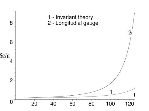
Our calculations clearly prove that the use of an arbitrariness in the co-ordinates selection for the interpretation of physical effects is incorrect. In the longitudinal gauge together with real physical effects there are the effects, caused by motion of the frame of reference within the gauge. Selection and removing of such nonphysical coordinate effects is possible only in the framework of invariant approach. At Fig. 2 one has shown the qualitative comparison of long-wave energy density perturbations calculated at the inflationary stage in the both approaches. We have used the simplest model with the potential (4) in the case $m=0.15,\;H_{0}=1,\;\tilde{a}_{0}=1$. Analytical expressions for $\delta\varepsilon_{inv}/\varepsilon$ are shown in Appendix.

Figure 2: Long-wave perturbations of energy density calculated at the inflationary stage in the both approaches – in the invariant theory (1) and by using the longitudinal gauge (2).

But if in principle we can analyze the long-wave metric perturbations in the longitudinal gauge, because we know a form of nonphysical terms (93), then the similar analysis of the short-wave perturbations in this gauge is absolutely impossible. Let’s consider this problem in detail.

Invariant theory gives the single expression for nonphysical terms (93), which is correct for all wave lengths. Therefore in the longitudinal gauge the expression

$$\frac{\delta\varepsilon_{inv}}{\varepsilon}=-\frac{2}{3H^{2}}\frac{k^{2}}{a^{2}}\Phi_{\bf k}-\frac{2\dot{\Phi}_{\bf k}}{H}-2\Phi_{\bf k}-2\frac{\dot{H}}{H}\int\limits_{t_{0}}^{t}\Phi_{\bf k}dt$$ (97)

is an invariant thus it should be correct the following expression

$$-\frac{2}{3H^{2}}\frac{k^{2}}{a^{2}}\delta\Phi_{\bf k}-\frac{2\dot{(\delta\Phi_{\bf k})}}{H}-2\delta\Phi_{\bf k}-2\frac{\dot{H}}{H}\int\limits_{t_{0}}^{t}\delta\Phi_{\bf k}dt\equiv 0,$$ (98)

where $\delta\Phi_{\bf k}$ is the metric change in transition to the new frame of reference with the gauge conservation. At the same time a function $\delta\Phi_{\bf k}$ has to satisfy the equation (90). We have shown that the last condition does not hold for short waves.

Let us denote $\delta\Phi_{\bf k}=\Omega$ and consider the relation (98) as equation for $\Omega$

$$\dot{\Omega}+\frac{1}{3H}\frac{k^{2}}{a^{2}}\Omega+H\Omega+\dot{H}\int\limits_{t_{0}}^{t}\Omega dt=0.$$

We divide it now by $\dot{H},$ differentiate, and then multiply by $\dot{H}$. As a result we have the equation

$$\ddot{\Omega}+\dot{\Omega}\left(H-\frac{\ddot{H}}{\dot{H}}\right)+\Omega\left(2\dot{H}-\frac{H\ddot{H}}{\dot{H}}\right)+\dot{H}\frac{d}{dt}\left(\frac{1}{3H\dot{H}}\frac{k^{2}}{a^{2}}\Omega\right)=0,$$

which differs from equation for metric perturbations in the longitudinal gauge (90) by the term containing ${k^{2}}/{a^{2}}$. What is the reason? Probably the longitudinal gauge is restricted itself and an important information inevitably is lost in transition to this gauge.

Results of SIG-waves investigations fulfilled in the various gauges are substantially different. For example, in the synchronous gauge we have Grisch :

$$\begin{array}[]{c}\displaystyle ds^{2}=-a^{2}[d\eta^{2}-(\delta_{\alpha\beta}+h_{\alpha\beta})dx^{\alpha}dx^{\beta}],\\[14.22636pt] \displaystyle g_{00}=-a^{2},\;g_{0\alpha}=0,\;g_{\alpha\beta}=a^{2}[(1+hG)\delta_{\alpha\beta}+h_{l}k^{2}G_{,\alpha,\beta}],\end{array}$$ (101)

where $G$ is the scalar function defined in the 3-space. It satisfies equation ${G^{,\alpha}}_{,\alpha}+k^{2}G=0$. Since $h^{0}_{0}\equiv Q_{{\bf k}}=0,$ the non-invariant part of full perturbations of energy density (85) is equal to zero for any co-ordinates transformations preserving the gauge and thus the calculation of $\delta\varepsilon/\varepsilon$ gives a proper result in the synchronous gauge in contrast to the longitudinal one.

The closed system of equations for metric perturbations $h$ and $h_{l}$ is obtained by Grischuk Grisch . The equation for $h$ is the third order differential equation and it contains the nonphysical solution $h\sim H$, which may be obtained by the coordinate transformations preserving the gauge (101). Note that this solution is trivial for the same equation but written in terms of invariant (71), and it is easily to show that this equation coincides with the equation of invariant dynamics (81).

Now let us to say some words about the quantum perturbation theory as it is. First of all, notice, there is a formal problem in the theory: what function is the object of quantization. The pose of this problem is induced by our understanding that the coordinate effects that can be eliminated by the appropriate choice of a classical frame of reference must not to be subject to quantization. In the longitudinal gauge theory the discussion of this problem is again reduced to the question whether the description in terms of the relativistic potential is invariant or not. One of the achievements of our invariant theory is that this question is uniquely solved. Only the invariant metric function which is uniquely connected with the invariant characteristics of the inflaton field is the subject of quantization. For the short- wave-length metric fluctuations the normalization of quantum operator is easy to find:

$$\hat{J}_{\bf k}\approx\frac{3\dot{\varphi}}{H}\hat{\Psi}_{\bf k},\quad\hat{\Psi}_{\bf k}\approx\frac{1}{\sqrt{2k}a}\left[\hat{c}_{\bf k}\exp\int\limits_{0}^{t}\frac{k\,dt}{a}+\hat{c}^{+}_{-{\bf k}}\exp\left(-\int\limits_{0}^{t}\frac{k\,dt}{a}\right)\right],$$ (102)

where $\hat{c}_{\bf k}$ and $\hat{c}^{+}_{-{\bf k}}$ are annihilation and creation operators in quantum field theory. Notice, expressions (102) are used only to specify the initial conditions; the quantum dynamics itself is described by the exact operator equation (81). The subject of calculations is the value of energy density fluctuations averaged over the Heisenberg vacuum specified in the beginning of the inflation:

$$\left|\frac{\delta\varepsilon_{{\bf k}\,{\rm inv}}}{\varepsilon}\right|\equiv\sqrt{\bigl{\langle}0|\left(\frac{\delta\varepsilon_{{\bf k}\,{\rm inv}}}{\varepsilon}\right)^{2}|0\bigr{\rangle}}.$$ (103)

In order to calculate the value (103) one can solve equation (81) under $|c_{\bf k}|=|c_{-{\bf k}}^{+}|=1/2$. The averaging over the phases of the complex numbers $c_{\bf k}$, $c_{-{\bf k}}$ and taking the absolute value corresponds to the procedure of quantum averaging (see Appendix).

V Analytical investigation of the EID.

At the postinflationary stage the Hubble function $H(t)$ oscillates and there are points where $\dot{H}=0$. Thus formally the EID (81) has to have the mathematical singularities that could be an obstacle in investigations both analytical and numerical. However the transformations of EID coefficients together with background equations for arbitrary potential (7) have shown an absence of the mathematical singularities in reality that has opened the possibility for analytical investigations of the EID. This internal property of the invariant dynamics is its significant advantage.

Let us introduce a new function $\Psi_{{\bf k}}(t)$, related with invariant $J_{{\bf k}}(t)$ by relation:

$$J_{{\bf k}}=\frac{3\sqrt{-\dot{H}}}{H}\Psi_{{\bf k}}.$$ (104)

Equation for $\Psi_{{\bf k}}(t)$ has a form:

$$\begin{array}[]{l}\displaystyle\ddot{\Psi}_{\bf k}+3H\dot{\Psi}_{{\bf k}}+\left(\frac{k^{2}}{a^{2}}+\frac{1}{4}\frac{\ddot{H}^{2}}{\dot{H}^{2}}-\frac{1}{2}\frac{\stackrel{{\scriptstyle...}}{{H}}}{\dot{H}}+2\frac{\ddot{H}}{H}-2\frac{\dot{H}^{2}}{H^{2}}-\frac{3}{2}\frac{H\ddot{H}}{\dot{H}}+3\dot{H}\right)\Psi_{\bf k}=0.\end{array}$$ (106)

This equation is more convenient for analysis than initial (81), since all terms with singularities are concentrated in the single coefficient by $\Psi_{{\bf k}}$.

Now let us consider the elimination mechanism of these singularities in detail. The background system (7) for arbitrary potential can be written in the form

$$\begin{array}[]{l}\displaystyle\dot{H}=-\frac{\varkappa}{2}\dot{\varphi}^{2},\\[14.22636pt] \displaystyle\ddot{\varphi}+3H\dot{\varphi}+\frac{\partial U(\varphi)}{\partial\varphi}=0.\end{array}$$

First equation has to be differentiated with respect to $t$ twice, the second one – once, then obtained expression has to be multiplied by $\varkappa\dot{\varphi}$. As a result we have the following necessary relations:

$$\begin{array}[]{l}\displaystyle\dot{H}=-\frac{\varkappa}{2}\dot{\varphi}^{2},\quad\ddot{H}=-\varkappa\dot{\varphi}\ddot{\varphi},\quad\stackrel{{\scriptstyle...}}{{H}}=-\varkappa\dot{\varphi}\ddot{\varphi}^{2}-\varkappa\dot{\varphi}\stackrel{{\scriptstyle...}}{{\varphi}},\\[14.22636pt] \displaystyle\varkappa\dot{\varphi}\stackrel{{\scriptstyle...}}{{\varphi}}+3\varkappa\dot{\varphi}^{2}\dot{H}+3\varkappa\dot{\varphi}\ddot{\varphi}H+\varkappa\dot{\varphi}^{2}\frac{\partial^{2}U(\varphi)}{\partial\varphi^{2}}=0.\end{array}$$

Expressing from first three relations the all derivatives of function $\varphi$ through derivatives of $H$ and substituting their to the forth one, after division by $2\dot{H}$ we obtain the following identity:

$$\frac{1}{4}\frac{\ddot{H}^{2}}{\dot{H}^{2}}-\frac{1}{2}\frac{\stackrel{{\scriptstyle...}}{{H}}}{\dot{H}}-3\dot{H}-\frac{3}{2}\frac{H\ddot{H}}{\dot{H}}\equiv\frac{\partial^{2}U(\varphi)}{\partial\varphi^{2}}.$$ (107)

Evidently, the structure of background equations allows to combine the terms with singularities into the smooth function that is the singularities cancel. Taking into account (107) the EID gains the simple form:

$$\ddot{\Psi}_{\bf k}+3H\dot{\Psi}_{{\bf k}}+\left(\frac{k^{2}}{a^{2}}+\frac{\partial^{2}U}{\partial\varphi^{2}}+2\frac{\ddot{H}}{H}-2\frac{\dot{H}^{2}}{H^{2}}+6\dot{H}\right)\Psi_{\bf k}=0.$$ (108)

One can rewrite its in the form:

$$\ddot{\Psi}_{\bf k}+3H\dot{\Psi}_{{\bf k}}+\left(\frac{k^{2}}{a^{2}}+U^{\prime\prime}_{\varphi\varphi}+\rho(t)\right)\Psi_{\bf k}=0,$$ (109)

where $U^{\prime\prime}_{\varphi\varphi}\equiv\frac{\partial^{2}U}{\partial\varphi^{2}},$ $\rho(t)\equiv\frac{d}{dt}\left(2\frac{\dot{H}}{H}+6H\right).$

Let us introduce the characteristic function

$$q(k,t)=\frac{k^{2}}{a^{2}(U^{\prime\prime}_{\varphi\varphi}(\varphi(t))+\rho(t))}.$$

Function $q(k,t)$ has a substantially different form at various stages of evolution but at the all applicable domain $t\in(0\;.\,.\;\infty)$ it decreases with the time growth. There are three types of metric perturbations depending on value $q(k,t)$:

1. Asymptotically long-wave perturbations, if

   $$q(k,t)\ll 1;$$ (110)

2. Perturbations of middle wave lengths, if:

   $$q(k,t)\sim 1;$$ (111)

3. Asymptotically short-wave perturbations, if

   $$q(k,t)\gg 1.$$ (112)

Consider the long-wave limit (110). The equation of invariant dynamics (108) in this limit reads

$$\ddot{\Psi}_{\bf k}+3H\dot{\Psi}_{{\bf k}}+\left(\frac{\partial^{2}U}{\partial\varphi^{2}}+2\frac{\ddot{H}}{H}-2\frac{\dot{H}^{2}}{H^{2}}+6\dot{H}\right)\Psi_{\bf k}=0.$$ (113)

Taking into account (107) it is easily to show that $\Psi_{{\bf k}}(t)=\sqrt{-\dot{H}}/H$ is the particular solution of this equation. Therefore the general solution of the EID for long waves with the arbitrary potential $U(\varphi)$ has a form:

$$\Psi_{{\bf k}}(t)=C_{1}\frac{\sqrt{-\dot{H}}}{H}+C_{2}\frac{\sqrt{-\dot{H}}}{H}\int_{0}^{t}\frac{H^{2}}{\dot{H}a^{3}}dt.$$ (114)

Deeper analysis is possible only in the framework of fixed potential. Further calculations are fulfilled for the simplest inflation model with the potential (4). In this model function $\Psi_{{\bf k}}$ for long-wave metric perturbations at the postinflationary stage oscillates with the stationary amplitude:

$$\Psi_{{\bf k}}(t)\sim\sin(m(t-t_{0})+\alpha/2),$$ (115)

where $\alpha$ is defined in (25). This result may be also obtained by direct solution of the EID which in that case reduces to the Matieu-like equation where there is a time-dependent coefficient by the oscillating correction in the frequency. Within that context the form of relation (115) means the presence of the parametric resonance for long-wave metric perturbations at the postinflationary stage.

Let’s return to initial equation (109) and proceed to the conformal time $\eta$:

$$\Psi^{\prime\prime}_{\bf k}+2\frac{a^{\prime}}{a}\Psi^{\prime}_{\bf k}+(k^{2}+a^{2}U^{\prime\prime}_{\varphi\varphi}+a^{2}\rho(\eta))\Psi_{\bf k}=0.$$ (116)

By substitution $\Psi_{\bf k}=\xi\Psi_{{\bf k}}^{0}$, where $\xi$ is a new unknown function, $\Psi_{{\bf k}}^{0}=\sqrt{-\dot{H}}/H$ is the particular long wave solution, this equation is reduced to

$$\xi^{\prime\prime}+2\xi^{\prime}\frac{(a\Psi_{{\bf k}}^{0})^{\prime}}{a\Psi_{{\bf k}}^{0}}+k^{2}\xi=0.$$ (117)

At the inflationary stage this equation can be reduced to the Bessel equation for any $k$:

$$\xi^{\prime\prime}-2\frac{\left(1+\frac{m^{2}}{3H^{2}}\right)}{\eta}\xi^{\prime}+k^{2}\xi=0.$$

Its exact solution is

$$\xi(\eta)=\eta^{\left(1+\frac{m^{2}}{3H^{2}}+\frac{1}{2}\right)}\left[C_{1}\,\mathrm{BesselY}\left(1+\frac{m^{2}}{3H^{2}}+\frac{1}{2},k\eta\right)+C_{2}\,\mathrm{BesselJ}\left(1+\frac{m^{2}}{3H^{2}}+\frac{1}{2},k\eta\right)\right].$$

At the most part of inflationary stage the inequality $\frac{m^{2}}{3H^{2}}\ll 1$ is valid. In this case we have

$$\xi(\eta)=L_{1}(k\eta\cos(k\eta)-\sin(k\eta))+L_{2}(k\eta\sin(k\eta)+\cos(k\eta)).$$

Therefore the general solution of the EID at the inflationary stage has a form

$$\begin{array}[]{l}\displaystyle\Psi_{\bf k}(t)=L_{1}\frac{\sqrt{-\dot{H}}}{H}\left(\int\frac{k}{a}dt\;\cos\left(\int\frac{k}{a}dt\right)-\sin\left(\int\frac{k}{a}dt\right)\right)+\\[14.22636pt] \displaystyle+L_{2}\frac{\sqrt{-\dot{H}}}{H}\left(\int\frac{k}{a}dt\;\sin\left(\int\frac{k}{a}dt\;\right)+\cos\left(\int\frac{k}{a}dt\right)\right).\end{array}$$ (120)

Entry conditions for $\Psi_{\bf k}(t)$

$$\Psi_{{\bf k}_{0}}=\sqrt{\frac{\varkappa}{2k}}\frac{1}{\tilde{a}_{0}},\quad\dot{\Psi}_{{\bf k}_{0}}=\sqrt{\frac{\varkappa k}{2}}\frac{1}{\tilde{a}_{0}^{2}}$$

give the following expressions for integration constants $L_{1}$ and $L_{2}$:

$$L_{1}=-H_{0}^{2}\sqrt{\frac{3\varkappa}{2}}\frac{\cos(k\eta_{0})-\sin(k\eta_{0})}{mk^{3/2}},\quad L_{2}=-H_{0}^{2}\sqrt{\frac{3\varkappa}{2}}\frac{\cos(k\eta_{0})+\sin(k\eta_{0})}{mk^{3/2}},$$ (121)

where

$$\eta_{0}\equiv\eta(t=0)=\int\frac{dt}{a}\biggr{|}_{t=0}\approx-\frac{1}{\tilde{a}_{0}H_{0}}.$$

The equation $q(k,t)=1$ represents relation between $k$ and $t$ at the boundary that separates the evolutional stages. Its solution $\tilde{t}(k)$ is the time of transition from short waves to long ones for every $k$. There are two variants depending on $k$:

1. The transition from short-wave perturbations to long-wave ones occurs at the inflationary stage that is $0<\tilde{t}(k)<t_{1}$;

2. The transition from short-wave perturbations to long-wave ones occurs at the postinflationary stage that is $\tilde{t}(k)>t_{1}$.

For every variant the EID (108) at the postinflationary stage should be solved separately.

In the first case at the times $t>t_{1}$ there are long-wave metric perturbations described by (114) or (115). After matching with solution (120) at the moment $t_{1}$ when the inflation terminates, we obtain

$$\Psi_{{\bf k}}(t)=-H_{0}^{2}\sqrt{\frac{3\varkappa}{2}}\frac{\cos(k\eta_{0})+\sin(k\eta_{0})}{mk^{3/2}}\frac{\sqrt{-\dot{H}}}{H}.$$ (122)

Finally consider the second particular case. The short-wave solution at the inflationary stage is (120). Let us obtain the short-wave solution at the postinflationary stage. Let us introduce a new function $\phi=a\Psi_{\bf k}$ into the (116). Using (29), we get

$$\phi^{\prime\prime}+\phi\left(k^{2}-\frac{2}{\eta^{2}}+\frac{m^{2}A^{6}}{81}\eta^{4}-\frac{4mA^{3}}{3}\eta\sin\left(\frac{2mA^{3}}{27}\eta^{3}+\beta\right)\right)=0.$$ (123)

In the short-wave limit on right $t\rightarrow t_{1}$ this equation can be simplified:

$$\phi^{\prime\prime}+\phi\left(k^{2}+\frac{m^{2}A^{6}}{81}\eta^{4}\right)=0.$$ (124)

Obviously this equation is an oscillator-like equation and it should be solved by the asymptotic method which has described in the Section 2. One has obtained the following general asymptotic solution:

$$\begin{array}[]{l}\displaystyle\Psi_{\bf k}(t)=\frac{1}{(t-t_{0})^{2/3}\sqrt{1+\frac{m^{4/3}}{2p^{2}}(t-t_{0})^{4/3}-\frac{3m^{8/3}}{8p^{4}}(t-t_{0})^{8/3}}}\times\\[14.22636pt] \displaystyle\times\biggl{[}M_{1}\cos\left(3pm^{1/3}(t-t_{0})^{1/3}+\frac{3m^{5/3}}{10p}(t-t_{0})^{5/3}-\frac{m^{3}}{8p^{3}}(t-t_{0})^{3}\right)+\\[14.22636pt] \displaystyle M_{2}\sin\left(3pm^{1/3}(t-t_{0})^{1/3}+\frac{3m^{5/3}}{10p}(t-t_{0})^{5/3}-\frac{m^{3}}{8p^{3}}(t-t_{0})^{3}\right)\biggr{]},\quad\mathrm{where}\;p=p(k),\end{array}$$ (128)

$$\begin{array}[]{l}\displaystyle M_{1}=-\frac{1}{m^{2/3}}\sqrt{\frac{2\varkappa}{p}}\frac{18H_{0}^{2}}{{\tilde{a}_{0}}^{3/2}m^{5/2}exp\left(\frac{9H_{0}^{2}}{4m^{2}}\right)}\left[\cos\left(\frac{pme^{\frac{3H_{0}^{2}}{2m^{2}}}}{2^{2/3}H_{0}}\right)+\sin\left(\frac{pme^{\frac{3H_{0}^{2}}{2m^{2}}}}{2^{2/3}H_{0}}\right)\right],\\[14.22636pt] \displaystyle M_{2}=-\frac{1}{m^{2/3}}\sqrt{\frac{2\varkappa}{p}}\frac{18H_{0}^{2}}{{\tilde{a}_{0}}^{3/2}m^{5/2}exp\left(\frac{9H_{0}^{2}}{4m^{2}}\right)}\left[\cos\left(\frac{pme^{\frac{3H_{0}^{2}}{2m^{2}}}}{2^{2/3}H_{0}}\right)-\sin\left(\frac{pme^{\frac{3H_{0}^{2}}{2m^{2}}}}{2^{2/3}H_{0}}\right)\right].\end{array}$$ (131)

The equation (108) for function $\chi=\Psi_{\bf k}(t-t_{0})$ has a form:

$$\chi^{\prime\prime}+\left(1+\frac{p^{2}}{\tau^{4/3}}-\frac{4}{\tau}\sin(2\tau+\alpha)\right)\chi=0.$$ (132)

Here $\tau=m(t-t_{0})$ is the new dimensionless variable. Depending on $\tau$ part of frequency

$$\rho(\tau)=\frac{p^{2}}{\tau^{4/3}}-\frac{4}{\tau}\sin(2\tau+\alpha),\quad\rho(\tau)\rightarrow 0\quad\mathrm{for}\quad\tau\rightarrow\infty$$

contains both monotonous and oscillating constituents thus this equation differs from both the oscillator-like equation and the Mathieu-like equation.

With the time growth the term ${p^{2}}/{\tau^{4/3}}$ drops faster then the absolute value of $(4/\tau)\sin(2\tau+\alpha)$. The condition of their equality gives an estimation of the lower time border for the asymptotically long waves:

$$\frac{p^{2}}{\tau_{long}^{4/3}}\sim\frac{1}{\tau_{long}}\;\longrightarrow\;\tau_{long}\sim p^{6}.$$ (133)

From (132) one can estimate also the upper time border of the asymptotically short waves:

$$\frac{p^{2}}{\tau_{short}^{4/3}}\sim 1\;\longrightarrow\;\tau_{short}\sim p^{3/2}.$$ (134)

The interval

$$\Delta\tau=p^{6}-p^{3/2}$$

gives an estimation of the transition duration between asymptotic waves.

We have developed the special asymptotic method which allows us to receive the asymptotic solution of equations like

$$y^{\prime\prime}+\left(1+\frac{const}{x^{n}}+\frac{4}{x^{m}}\sin(2x+\alpha)\right)=0$$

with any desired order of accuracy. Formal scheme for construction of general solution is similar with one for Mathieu-like equation. At first we don’t take into account the oscillating correction and solve the oscillator-like equation. Then we add the mixed harmonics into the solution, all constants before trigonometrical functions replace by functions in the form of power series that depends on $n$ and $m$, so the whole problem reduces to search of expansion coefficients.

Let us apply this scheme to equation (132). We solve the oscillator-like equation

$$\chi^{\prime\prime}+\left(1+\frac{p^{2}}{\tau^{4/3}}\right)\chi=0.$$

Here $p^{2}/\tau^{4/3}\rightarrow 0$ steadily in the limit $\tau\rightarrow\infty$, therefore the general asymptotic method is applicable for solution of this equation (see Section 2). So we have

$$\chi(\tau)=\frac{1}{\sqrt{1+\frac{p^{2}}{2\tau^{4/3}}}}\left[C_{1}e^{-i\left(\tau-\frac{3p^{2}}{2\tau^{1/3}}\right)}+C_{2}e^{i\left(\tau-\frac{3p^{2}}{2\tau^{1/3}}\right)}\right].$$ (135)

Now let’s take into account the influence of correction $(4/\tau)\sin(2\tau+\alpha)$. Equation (132) one can write in a form

$$\chi^{\prime\prime}+\left(1+\frac{p^{2}}{\tau^{4/3}}+\frac{2i}{\tau}e^{i(2\tau+\alpha)}-\frac{2i}{\tau}e^{-i(2\tau+\alpha)}\right)\chi=0.$$ (136)

According to described scheme the general form of solution in the limit $\tau\rightarrow\infty$ is

$$\begin{array}[]{l}\displaystyle\chi(\tau)=\frac{1}{\sqrt{1+\frac{p^{2}}{2\tau^{4/3}}}}\sum_{s=0}^{\infty}\biggl{[}A_{s}(\tau)e^{i(2s+1)(\tau+\alpha/2)}e^{i\left(\frac{3p^{2}}{2\tau^{1/3}}+\varphi_{1}\right)}+B_{s}(\tau)e^{-i(2s+1)(\tau+\alpha/2)}e^{-i\left(\frac{3p^{2}}{2\tau^{1/3}}+\varphi_{2}\right)}+\\[14.22636pt] \displaystyle+C_{s}(\tau)e^{i(2s+1)(\tau+\alpha/2)}e^{-i\left(\frac{3p^{2}}{2\tau^{1/3}}+\varphi_{2}\right)}+D_{s}(\tau)e^{-i(2s+1)(\tau+\alpha/2)}e^{i\left(\frac{3p^{2}}{2\tau^{1/3}}+\varphi_{1}\right)}\biggr{]},\end{array}$$ (139)

where $\varphi_{1},\;\varphi_{2}$ = const. In the frequency of equation (136) there are the terms with powers of $\tau$ multiple to $1/3$. Therefore

$$\begin{array}[]{l}\displaystyle A_{s}(\tau)=\sum_{k=3}^{-\infty}a_{sk}\tau^{k/3},\quad B_{s}(\tau)=\sum_{k=3}^{-\infty}b_{sk}\tau^{k/3},\\[14.22636pt] \displaystyle C_{s}(\tau)=\sum_{k=3}^{-\infty}c_{sk}\tau^{k/3},\quad D_{s}(\tau)=\sum_{k=3}^{-\infty}d_{sk}\tau^{k/3}.\end{array}$$ (142)

For a function $\Psi_{\bf k}(t)=\chi/(t-t_{0})$ we have obtained the following expression:

$$\begin{array}[]{l}\displaystyle\Psi_{\bf k}(t)=\frac{C_{1}}{\sqrt{1+\frac{p^{2}}{2m^{4/3}(t-t_{0})^{4/3}}}}\biggl{[}\biggl{(}\left(\frac{1}{t-t_{0}}-\frac{20m^{2/3}}{3p^{4}(t-t_{0})^{1/3}}\right)\sin\left(\frac{3p^{2}}{2m^{1/3}(t-t_{0})^{1/3}}\right)-\\[14.22636pt] \displaystyle-\left(\frac{40m}{9p^{6}}-\frac{4m^{1/3}}{p^{2}(t-t_{0})^{2/3}}\right)\cos\left(\frac{3p^{2}}{2m^{1/3}(t-t_{0})^{1/3}}\right)\biggr{)}\sin(m(t-t_{0})+\alpha/2)+\\[14.22636pt] \displaystyle+\left(-\frac{2m^{1/3}}{p^{2}(t-t_{0})^{2/3}}\sin\left(\frac{3p^{2}}{2m^{1/3}(t-t_{0})^{1/3}}\right)+\left(\frac{1}{t-t_{0}}-\frac{4m^{2/3}}{3p^{4}(t-t_{0})^{1/3}}\right)\cos\left(\frac{3p^{2}}{2m^{1/3}(t-t_{0})^{1/3}}\right)\right)\times\\[14.22636pt] \displaystyle\times\cos(m(t-t_{0})+\alpha/2)\biggr{]}+\end{array}$$ (147)

$$\begin{array}[]{l}\displaystyle\qquad\quad\;+\frac{C_{2}}{\sqrt{1+\frac{p^{2}}{2m^{4/3}(t-t_{0})^{4/3}}}}\biggl{[}\biggl{(}\left(\frac{20m^{2/3}}{3p^{4}(t-t_{0})^{1/3}}-\frac{1}{t-t_{0}}\right)\cos\left(\frac{3p^{2}}{2m^{1/3}(t-t_{0})^{1/3}}\right)-\\[14.22636pt] \displaystyle-\left(\frac{40m}{9p^{6}}-\frac{4m^{1/3}}{p^{2}(t-t_{0})^{2/3}}\right)\sin\left(\frac{3p^{2}}{2m^{1/3}(t-t_{0})^{1/3}}\right)\biggr{)}\sin(m(t-t_{0})+\alpha/2)+\\[14.22636pt] \displaystyle+\left(\frac{2m^{1/3}}{p^{2}(t-t_{0})^{2/3}}\cos\left(\frac{3p^{2}}{2m^{1/3}(t-t_{0})^{1/3}}\right)+\left(\frac{1}{t-t_{0}}-\frac{4m^{2/3}}{3p^{4}(t-t_{0})^{1/3}}\right)\sin\left(\frac{3p^{2}}{2m^{1/3}(t-t_{0})^{1/3}}\right)\right)\times\\[14.22636pt] \displaystyle\times\cos(m(t-t_{0})+\alpha/2)\biggr{]},\end{array}$$

where $\alpha$ is defined in (25). Constants $C_{1}$ and $C_{2}$ are found by matching of solution (147) with the short-wave solution (128). The matching time is defined from relation (134):

$$\tilde{t}(k)=\frac{p^{3/2}}{m}+t_{0}.$$ (148)

Therefore

$$\begin{array}[]{l}\displaystyle\qquad\quad\;C_{1}=-\sqrt{\frac{3\varkappa}{2}}\frac{3H_{0}^{2}}{exp\left(\frac{9H_{0}^{2}}{4m^{2}}\right)m^{7/2}{\tilde{a}_{0}}^{3/2}}\biggl{[}\cos\left(-\frac{\alpha}{2}-\frac{107}{40}p^{3/2}-\frac{1}{2^{2/3}H_{0}}pme^{\frac{3H_{0}^{2}}{2m^{2}}}\right)-\\[22.76219pt] \displaystyle\sin\left(-\frac{\alpha}{2}-\frac{107}{40}p^{3/2}-\frac{1}{2^{2/3}H_{0}}pme^{\frac{3H_{0}^{2}}{2m^{2}}}\right)+7\cos\left(\frac{\alpha}{2}-\frac{147}{40}p^{3/2}-\frac{1}{2^{2/3}H_{0}}pme^{\frac{3H_{0}^{2}}{2m^{2}}}\right)\\[22.76219pt] \displaystyle-7\sin\left(\frac{\alpha}{2}-\frac{147}{40}p^{3/2}-\frac{1}{2^{2/3}H_{0}}pme^{\frac{3H_{0}^{2}}{2m^{2}}}\right)\biggr{]}\;;\end{array}$$ (152)

$$\begin{array}[]{l}\displaystyle\qquad\quad\;C_{2}=-\sqrt{\frac{3\varkappa}{2}}\frac{3H_{0}^{2}}{exp\left(\frac{9H_{0}^{2}}{4m^{2}}\right)m^{7/2}{\tilde{a}_{0}}^{3/2}}\biggl{[}-7\sin\left(\frac{\alpha}{2}-\frac{147}{40}p^{3/2}-\frac{1}{2^{2/3}H_{0}}pme^{\frac{3H_{0}^{2}}{2m^{2}}}\right)-\\[22.76219pt] \displaystyle 7\cos\left(\frac{\alpha}{2}-\frac{147}{40}p^{3/2}-\frac{1}{2^{2/3}H_{0}}pme^{\frac{3H_{0}^{2}}{2m^{2}}}\right)+\sin\left(-\frac{\alpha}{2}-\frac{107}{40}p^{3/2}-\frac{1}{2^{2/3}H_{0}}pme^{\frac{3H_{0}^{2}}{2m^{2}}}\right)\\[22.76219pt] \displaystyle+\cos\left(-\frac{\alpha}{2}-\frac{107}{40}p^{3/2}-\frac{1}{2^{2/3}H_{0}}pme^{\frac{3H_{0}^{2}}{2m^{2}}}\right)\biggr{]}.\end{array}$$

Function of metric perturbations (147) for every regime can be essentially simplified:

1) Transient regime at $\tilde{t}(k)\lesssim t<t_{long},$ where $t_{long}={p^{6}}/{m}+t_{0}$:

$$\Psi_{\bf k}\approx\frac{C_{1}\cos\left(\frac{3p^{2}}{2m^{1/3}(t-t_{0})^{1/3}}-m(t-t_{0})-\frac{\alpha}{2}\right)+C_{2}\sin\left(\frac{3p^{2}}{2m^{1/3}(t-t_{0})^{1/3}}-m(t-t_{0})-\frac{\alpha}{2}\right)}{(t-t_{0})\sqrt{1+\frac{p^{2}}{2m^{4/3}(t-t_{0})^{4/3}}}}$$ (153)

2) Long-wave regime at $t>t_{long}$:

$$\Psi_{\bf k} \approx -\frac{40m}{9p^{6}}\sin\left(m(t-t_{0})+\frac{\alpha}{2}\right)\times$$ (154)

$$\times \left[C_{1}\cos\left(\frac{3p^{2}}{2m^{1/3}(t-t_{0})^{1/3}}\right)+C_{2}\sin\left(\frac{3p^{2}}{2m^{1/3}(t-t_{0})^{1/3}}\right)\right]$$

Last expression one can also write in the form analogous to (122):

$$\Psi_{\bf k}\approx-\frac{40m}{9\sqrt{3}p^{6}}\frac{\sqrt{-\dot{H}}}{H}\left(C_{1}\cos\left(\frac{3p^{2}}{2m^{1/3}(t-t_{0})^{1/3}}\right)+C_{2}\sin\left(\frac{3p^{2}}{2m^{1/3}(t-t_{0})^{1/3}}\right)\right).$$ (155)

Obviously the function of long-wave solution (154) oscillates with the constant amplitude as $\sin\left(m(t-t_{0})+{\alpha}/{2}\right)$, however, in contrast to (122), there is a slowly varying modulation factor, which approaches to the constant just in the limit $t\rightarrow\infty$.

Theoretical predictions for the parameter of energy density perturbations spectrum are of the most interest. This parameter is defined as follows

$$\Delta=\left(\bigl{\langle}0|\left(\frac{\delta\varepsilon_{{\bf k}\,{\rm inv}}}{\varepsilon}\right)^{2}|0\bigr{\rangle}\frac{k^{3}}{2\pi^{2}}\right)^{1/2}.$$ (156)

The analytical results of calculation of $\Delta$ without the averaging over the initial phases of quantum fluctuations are shown in Appendix.

VI Conclusion.

Gauge invariant approach to investigation of linear scalar perturbations of inflaton and gravitational fields (SIG-waves) has been developed. We mean the derivation and analytical investigation of equation for the single invariant function $J_{{\bf k}}$ without resorting any gauge. Equation of invariant dynamics (EID) is constructed both in the cosmic and conformal times. The transformations of EID coefficients together with background equations for arbitrary potential have shown an absence of the mathematical singularities in reality. This fact has given a chance for analytical investigations of the EID. This internal property of the invariant dynamics is its significant advantage.

Our approach allows to compare various gauges used by other researchers, and to find unambiguous selection criteria of physical and coordinate effects. We have shown that the so-called longitudinal gauge commonly used for studying the gravitational instability leads to the overestimation of physical effects due to presence of nonphysical proper time perturbations in results obtained by using this gauge.

We have proven that the non-invariant part of energy density perturbations in the synchronous gauge is equal to zero for any co-ordinates transformations preserving the gauge, therefore the calculation of the relative perturbation of energy density $\delta\varepsilon/\varepsilon$ in the synchronous gauge gives correct results in contrast to the longitudinal one.

To a great extent, the technology of EID solving rests upon mathematical symmetry properties of invariant dynamics. The general long-wave solution of EID as a functional of background solution for arbitrary potential $U(\phi)$ is obtained. We have developed asymptotical methods which allow us to obtain the invariant function of metric perturbations in analytical form at all stages of the Universe evolution for arbitrary wave lengths in the framework of fixed potential (we use of the simplest model with $U(\varphi)=m^{2}\varphi^{2}/2$). It is important point of our investigation that both the non-perturbed or background characteristics (Hubble function $H(t),$ inflaton $\phi(t)$ and scalar factor $a(t)$) and characteristics of metric perturbations (invariant functions $J_{\bf k}$ or $\Psi_{\bf k}$) at the inflationary and postinflationary stages in the considering model (1) of the Universe are completely defined by parameter $m$ and initial values of Hubble function $H_{0}$ and scale factor $\tilde{a}_{0}.$ Note also that all analytical results coincide with numerical solution of EID at various stages and wave numbers with a high precision.

We have also obtained analytical expressions for the energy density perturbations spectrum $\Delta(k,t)$ for all possible wave numbers $k$ and times $t.$ (see Appendix). Amplitude of the long-wave spectrum in the case of transition from short waves to long ones occurs at the inflationary stage is almost flat, i.e. has the Harrison-Zeldovich form, for arbitrary potential $U(\varphi),$ but there is some tilt that can be compared with one from recent high precision data. This result is supposed to be the principal result of our invariant approach. Inflationary prediction for nearly flat spectrum of density perturbations is in agreement with both measurements of the CMB anisotropy and observations of structures in the Universe.

We are grateful to V.A. Beylin, V.I. Kuksa, O.D. Lalakulich, L.S. Marochnik, A.V. Zayakin and O.V. Teryaev for useful discussions and comments. This work is partially supported by grant RFBR 03-02-16816.

VII Appendix. Calculation of the energy density perturbation spectrum.

In this section there are the analytical expressions for the parameter of energy density perturbations spectrum $\Delta(k,t)$ (156):

$$\Delta(k,t)=\frac{k^{3/2}}{\sqrt{2}\pi}\left|\frac{\delta\varepsilon_{inv}}{\varepsilon}\right|.$$ (157)

Expression for relative perturbations of energy density through $\Psi_{\bf k}$ has a form:

$$\frac{\delta\varepsilon_{inv}}{\varepsilon}=-\frac{\sqrt{-2\dot{H}}}{3H^{2}}\left[\dot{\Psi}_{\bf k}+\left(\frac{\dot{H}}{H}-3H-\frac{\ddot{H}}{2\dot{H}}\right)\Psi_{\bf k}\right]+\frac{\sqrt{2}\dot{H}}{H}\int\limits_{t_{0}}^{t}\frac{\sqrt{-\dot{H}}}{H}\Psi_{\bf k}dt.$$ (158)

Using the expressions for $\Psi_{\bf k}$ at various $t$ and $k$ (120), (122), (128), (153) and (155), we have obtained the following expressions for ${\delta\varepsilon_{inv}}/{\varepsilon}$ and $\Delta(k,t)$:

1. Short waves at the inflationary stage that is at times $0<t<\tilde{t}(k),\quad t\leqslant t_{1},$ where $\tilde{t}(k)$ is the transition time from short waves to long ones, $t_{1}$ is the time when the inflationary stage terminates. In that case we have

   $$\begin{array}[]{l}\displaystyle\frac{\delta\varepsilon_{inv}}{\varepsilon}=-\frac{2\sqrt{3\varkappa}mH_{0}^{2}}{9{H(t)}^{3}{\tilde{a}_{0}}^{2}(H_{0}+H(t))}k^{1/2}e^{-t(H_{0}+H(t))}\times\\[14.22636pt] \displaystyle\times\left[\cos\left(\frac{2ke^{-\frac{t(H_{0}+H(t))}{2}}}{(H_{0}+H(t))\tilde{a}_{0}}-\frac{k}{H_{0}\tilde{a}_{0}}\right)+\sin\left(\frac{2ke^{-\frac{t(H_{0}+H(t))}{2}}}{(H_{0}+H(t))\tilde{a}_{0}}-\frac{k}{H_{0}\tilde{a}_{0}}\right)\right];\end{array}$$ (161)

   $$\begin{array}[]{l}\displaystyle\Delta(k,t)=\frac{\sqrt{6\varkappa}mH_{0}^{2}}{9\pi{H(t)}^{3}{\tilde{a}_{0}}^{2}(H_{0}+H(t))}k^{2}e^{-t(H_{0}+H(t))}\times\\[14.22636pt] \displaystyle\times\left|\cos\left(\frac{2ke^{-\frac{t(H_{0}+H(t))}{2}}}{(H_{0}+H(t))\tilde{a}_{0}}-\frac{k}{H_{0}\tilde{a}_{0}}\right)+\sin\left(\frac{2ke^{-\frac{t(H_{0}+H(t))}{2}}}{(H_{0}+H(t))\tilde{a}_{0}}-\frac{k}{H_{0}\tilde{a}_{0}}\right)\right|.\end{array}$$ (164)

2. Long waves in the case of the transition from short waves to long ones occurs at the inflationary stage that is at times $t>\tilde{t}(k),\quad\tilde{t}(k)\leqslant t_{1}$. Here we have

   $$\frac{\delta\varepsilon_{inv}}{\varepsilon}=\frac{\sqrt{3\varkappa}H_{0}^{2}}{mH_{s}}\frac{\dot{H}(t)}{k^{3/2}H(t)}\left[\cos\left(\frac{k}{H_{0}\tilde{a}_{0}}\right)-\sin\left(\frac{k}{H_{0}\tilde{a}_{0}}\right)\right];$$ (165)

   $$\Delta(k,t)=-\sqrt{\frac{3\varkappa}{2}}\frac{H_{0}^{2}}{\pi mH_{s}}\frac{\dot{H}(t)}{H(t)}\left|\cos\left(\frac{k}{H_{0}\tilde{a}_{0}}\right)-\sin\left(\frac{k}{H_{0}\tilde{a}_{0}}\right)\right|,$$ (166)

   where

   $$H_{s}\equiv H(\tilde{t}(k))=\sqrt{{H_{0}}^{2}-\frac{2m^{2}}{3}\;\ln\left(\frac{k}{m\tilde{a}_{0}}\right)}$$

   is the value of Hubble function at the transition moment. We see that the amplitude of this spectrum is almost constant with $k$ for arbitrary potential $U(\varphi).$ Therefore this spectrum has the Harrison-Zeldovich form. Some tilt from flatness contains in $H_{s}$ and can be compared with recent high precision data.

3. Long waves in the case of the transition from short waves to long ones occurs at the postinflationary stage that is at times $t>t_{long},\quad t_{long}>t_{1}:$

   $$\begin{array}[]{l}\displaystyle\qquad\frac{\delta\varepsilon_{inv}}{\varepsilon}=-\frac{20\sqrt{\varkappa}H_{0}^{2}}{m^{7/2}{\tilde{a}_{0}}^{3/2}exp\left(\frac{9H_{0}^{2}}{4m^{2}}\right)}\frac{\dot{H}(t)}{H(t)}\biggl{[}\cos\left(\frac{3p^{2}}{2m^{1/3}(t-t_{0})^{1/3}}\right)\times\\[14.22636pt] \displaystyle\times\biggl{(}\cos\left(-\frac{\alpha}{2}-\frac{107}{40}p^{3/2}-\frac{1}{2^{2/3}H_{0}}pme^{\frac{3H_{0}^{2}}{2m^{2}}}\right)-\sin\left(-\frac{\alpha}{2}-\frac{107}{40}p^{3/2}-\frac{1}{2^{2/3}H_{0}}pme^{\frac{3H_{0}^{2}}{2m^{2}}}\right)+\\[14.22636pt] \displaystyle 7\cos\left(\frac{\alpha}{2}-\frac{147}{40}p^{3/2}-\frac{1}{2^{2/3}H_{0}}pme^{\frac{3H_{0}^{2}}{2m^{2}}}\right)-7\sin\left(\frac{\alpha}{2}-\frac{147}{40}p^{3/2}-\frac{1}{2^{2/3}H_{0}}pme^{\frac{3H_{0}^{2}}{2m^{2}}}\right)\biggr{)}+\end{array}$$ (170)

   $$\begin{array}[]{l}\displaystyle\qquad+\sin\left(\frac{3p^{2}}{2m^{1/3}(t-t_{0})^{1/3}}\right)\biggl{(}-7\sin\left(\frac{\alpha}{2}-\frac{147}{40}p^{3/2}-\frac{1}{2^{2/3}H_{0}}pme^{\frac{3H_{0}^{2}}{2m^{2}}}\right)-\\[14.22636pt] \displaystyle 7\cos\left(\frac{\alpha}{2}-\frac{147}{40}p^{3/2}-\frac{1}{2^{2/3}H_{0}}pme^{\frac{3H_{0}^{2}}{2m^{2}}}\right)+\sin\left(-\frac{\alpha}{2}-\frac{107}{40}p^{3/2}-\frac{1}{2^{2/3}H_{0}}pme^{\frac{3H_{0}^{2}}{2m^{2}}}\right)\\[14.22636pt] \displaystyle+\cos\left(-\frac{\alpha}{2}-\frac{107}{40}p^{3/2}-\frac{1}{2^{2/3}H_{0}}pme^{\frac{3H_{0}^{2}}{2m^{2}}}\right)\biggr{)}\biggr{]};\end{array}$$

   $$\begin{array}[]{l}\displaystyle\qquad\Delta(p,t)=-\frac{5\sqrt{2\varkappa}H_{0}^{2}}{\pi m^{2}}p^{3/2}\frac{\dot{H}(t)}{H(t)}\biggl{|}\cos\left(\frac{3p^{2}}{2m^{1/3}(t-t_{0})^{1/3}}\right)\times\\[14.22636pt] \displaystyle\times\biggl{(}\cos\left(-\frac{\alpha}{2}-\frac{107}{40}p^{3/2}-\frac{1}{2^{2/3}H_{0}}pme^{\frac{3H_{0}^{2}}{2m^{2}}}\right)-\sin\left(-\frac{\alpha}{2}-\frac{107}{40}p^{3/2}-\frac{1}{2^{2/3}H_{0}}pme^{\frac{3H_{0}^{2}}{2m^{2}}}\right)+\\[14.22636pt] \displaystyle 7\cos\left(\frac{\alpha}{2}-\frac{147}{40}p^{3/2}-\frac{1}{2^{2/3}H_{0}}pme^{\frac{3H_{0}^{2}}{2m^{2}}}\right)-7\sin\left(\frac{\alpha}{2}-\frac{147}{40}p^{3/2}-\frac{1}{2^{2/3}H_{0}}pme^{\frac{3H_{0}^{2}}{2m^{2}}}\right)\biggr{)}+\end{array}$$ (174)

   $$\begin{array}[]{l}\displaystyle\qquad+\sin\left(\frac{3p^{2}}{2m^{1/3}(t-t_{0})^{1/3}}\right)\biggl{(}-7\sin\left(\frac{\alpha}{2}-\frac{147}{40}p^{3/2}-\frac{1}{2^{2/3}H_{0}}pme^{\frac{3H_{0}^{2}}{2m^{2}}}\right)-\\[14.22636pt] \displaystyle 7\cos\left(\frac{\alpha}{2}-\frac{147}{40}p^{3/2}-\frac{1}{2^{2/3}H_{0}}pme^{\frac{3H_{0}^{2}}{2m^{2}}}\right)+\sin\left(-\frac{\alpha}{2}-\frac{107}{40}p^{3/2}-\frac{1}{2^{2/3}H_{0}}pme^{\frac{3H_{0}^{2}}{2m^{2}}}\right)\\[14.22636pt] \displaystyle+\cos\left(-\frac{\alpha}{2}-\frac{107}{40}p^{3/2}-\frac{1}{2^{2/3}H_{0}}pme^{\frac{3H_{0}^{2}}{2m^{2}}}\right)\biggr{)}\biggr{|}.\end{array}$$

   Here instead of $k$ we introduced a new parameter

   $$p=p(k)=\frac{2^{2/3}k}{\tilde{a}_{0}mexp\left(\frac{3H_{0}^{2}}{2m^{2}}\right)}\gg 2^{2/3}.$$

   Since these perturbations are considered at the postinflationary stage so in the framework of investigated model

   $$\frac{\dot{H}(t)}{H(t)}\approx-\frac{2}{t-t_{0}}\sin^{2}\left(m(t-t_{0})+\frac{\alpha}{2}\right).$$

   Apparently, the long-wave functions $\delta\varepsilon_{inv}/\varepsilon$ and $\Delta(k,t)$ are functionals of background solution $H(t)$ and depend on time as ${\dot{H}(t)}/{H(t)}$. This statement is correct for any potential.

4. Short waves at the postinflationary stage that is at times $t_{1}<t<\tilde{t}(k),\quad p\gg 2^{2/3}$:

   $$\begin{array}[]{l}\displaystyle\frac{\delta\varepsilon_{inv}}{\varepsilon}=-\sqrt{3\varkappa}\frac{9H_{0}^{2}}{m^{19/6}{\tilde{a}_{0}}^{3/2}exp\left(\frac{9H_{0}^{2}}{4m^{2}}\right)\sqrt{1+\frac{m^{4/3}}{2p^{2}}(t-t_{0})^{4/3}}}\times\\[14.22636pt] \displaystyle\times\biggl{[}\frac{p^{1/2}m^{1/3}}{(t-t_{0})^{1/3}}\biggl{(}\left(\cos\left(\frac{pm}{2^{2/3}H_{0}}e^{\frac{3H_{0}^{2}}{2m^{2}}}\right)+\sin\left(\frac{pm}{2^{2/3}H_{0}}e^{\frac{3H_{0}^{2}}{2m^{2}}}\right)\right)\times\\[14.22636pt] \displaystyle\times\left(\cos\left(m(t-t_{0})-3pm^{1/3}(t-t_{0})^{1/3}+\frac{\alpha}{2}\right)-\cos\left(m(t-t_{0})+3pm^{1/3}(t-t_{0})^{1/3}+\frac{\alpha}{2}\right)\right)-\\[14.22636pt] \displaystyle\qquad\qquad\quad-\left(\cos\left(\frac{pm}{2^{2/3}H_{0}}e^{\frac{3H_{0}^{2}}{2m^{2}}}\right)-\sin\left(\frac{pm}{2^{2/3}H_{0}}e^{\frac{3H_{0}^{2}}{2m^{2}}}\right)\right)\times\\[14.22636pt] \displaystyle\times\left(\sin\left(m(t-t_{0})+3pm^{1/3}(t-t_{0})^{1/3}+\frac{\alpha}{2}\right)+\sin\left(m(t-t_{0})-3pm^{1/3}(t-t_{0})^{1/3}+\frac{\alpha}{2}\right)\right)\biggr{)}+\end{array}$$ (180)

   $$\begin{array}[]{l}\displaystyle+\frac{m(t-t_{0})^{1/3}}{p^{1/2}}\biggl{(}\left(\cos\left(\frac{pm}{2^{2/3}H_{0}}e^{\frac{3H_{0}^{2}}{2m^{2}}}\right)+\sin\left(\frac{pm}{2^{2/3}H_{0}}e^{\frac{3H_{0}^{2}}{2m^{2}}}\right)\right)\times\\[14.22636pt] \displaystyle\times\left(\cos\left(m(t-t_{0})-3pm^{1/3}(t-t_{0})^{1/3}+\frac{\alpha}{2}\right)+\cos\left(m(t-t_{0})+3pm^{1/3}(t-t_{0})^{1/3}+\frac{\alpha}{2}\right)\right)+\\[14.22636pt] \displaystyle\qquad\qquad\qquad+\left(\cos\left(\frac{pm}{2^{2/3}H_{0}}e^{\frac{3H_{0}^{2}}{2m^{2}}}\right)-\sin\left(\frac{pm}{2^{2/3}H_{0}}e^{\frac{3H_{0}^{2}}{2m^{2}}}\right)\right)\times\\[14.22636pt] \displaystyle\times\left(\sin\left(m(t-t_{0})+3pm^{1/3}(t-t_{0})^{1/3}+\frac{\alpha}{2}\right)-\sin\left(m(t-t_{0})-3pm^{1/3}(t-t_{0})^{1/3}+\frac{\alpha}{2}\right)\right)\biggr{)}\biggr{]};\end{array}$$

   $$\begin{array}[]{l}\displaystyle\Delta(p,t)=\sqrt{\frac{3\varkappa}{2}}\frac{9H_{0}^{2}}{2\pi m^{5/3}\sqrt{1+\frac{m^{4/3}}{2p^{2}}(t-t_{0})^{4/3}}}\times\\[14.22636pt] \displaystyle\times\biggl{|}\frac{p^{2}m^{1/3}}{(t-t_{0})^{1/3}}\biggl{(}\left(\cos\left(\frac{pm}{2^{2/3}H_{0}}e^{\frac{3H_{0}^{2}}{2m^{2}}}\right)+\sin\left(\frac{pm}{2^{2/3}H_{0}}e^{\frac{3H_{0}^{2}}{2m^{2}}}\right)\right)\times\\[14.22636pt] \displaystyle\times\left(\cos\left(m(t-t_{0})-3pm^{1/3}(t-t_{0})^{1/3}+\frac{\alpha}{2}\right)-\cos\left(m(t-t_{0})+3pm^{1/3}(t-t_{0})^{1/3}+\frac{\alpha}{2}\right)\right)-\\[14.22636pt] \displaystyle\qquad\qquad\quad-\left(\cos\left(\frac{pm}{2^{2/3}H_{0}}e^{\frac{3H_{0}^{2}}{2m^{2}}}\right)-\sin\left(\frac{pm}{2^{2/3}H_{0}}e^{\frac{3H_{0}^{2}}{2m^{2}}}\right)\right)\times\\[14.22636pt] \displaystyle\times\left(\sin\left(m(t-t_{0})+3pm^{1/3}(t-t_{0})^{1/3}+\frac{\alpha}{2}\right)+\sin\left(m(t-t_{0})-3pm^{1/3}(t-t_{0})^{1/3}+\frac{\alpha}{2}\right)\right)\biggr{)}+\end{array}$$ (186)

   $$\begin{array}[]{l}\displaystyle+pm(t-t_{0})^{1/3}\biggl{(}\left(\cos\left(\frac{pm}{2^{2/3}H_{0}}e^{\frac{3H_{0}^{2}}{2m^{2}}}\right)+\sin\left(\frac{pm}{2^{2/3}H_{0}}e^{\frac{3H_{0}^{2}}{2m^{2}}}\right)\right)\times\\[14.22636pt] \displaystyle\times\left(\cos\left(m(t-t_{0})-3pm^{1/3}(t-t_{0})^{1/3}+\frac{\alpha}{2}\right)+\cos\left(m(t-t_{0})+3pm^{1/3}(t-t_{0})^{1/3}+\frac{\alpha}{2}\right)\right)+\\[14.22636pt] \displaystyle\qquad\qquad\qquad+\left(\cos\left(\frac{pm}{2^{2/3}H_{0}}e^{\frac{3H_{0}^{2}}{2m^{2}}}\right)-\sin\left(\frac{pm}{2^{2/3}H_{0}}e^{\frac{3H_{0}^{2}}{2m^{2}}}\right)\right)\times\\[14.22636pt] \displaystyle\times\left(\sin\left(m(t-t_{0})+3pm^{1/3}(t-t_{0})^{1/3}+\frac{\alpha}{2}\right)-\sin\left(m(t-t_{0})-3pm^{1/3}(t-t_{0})^{1/3}+\frac{\alpha}{2}\right)\right)\biggr{)}\biggr{|}.\end{array}$$

5. Waves of middle lengths (occurs only at the postinflationary stage) that is at times $t_{1}<\tilde{t}(k)<t<t_{long},\quad p\gg 2^{2/3}$:

   $$\begin{array}[]{l}\displaystyle\frac{\delta\varepsilon_{inv}}{\varepsilon}=-\sqrt{\varkappa}\frac{9H_{0}^{2}}{2m^{7/2}{\tilde{a}_{0}}^{3/2}exp\left(\frac{9H_{0}^{2}}{4m^{2}}\right)\sqrt{1+\frac{p^{2}}{2m^{4/3}(t-t_{0})^{4/3}}}}\times\\[22.76219pt] \displaystyle\times\biggl{[}\frac{p^{2}}{4m^{1/3}(t-t_{0})^{4/3}}\biggl{(}\biggl{[}\cos\left(-\frac{\alpha}{2}-\frac{107}{40}p^{3/2}-\frac{1}{2^{2/3}H_{0}}pme^{\frac{3H_{0}^{2}}{2m^{2}}}\right)-\\[22.76219pt] \displaystyle-\sin\left(-\frac{\alpha}{2}-\frac{107}{40}p^{3/2}-\frac{1}{2^{2/3}H_{0}}pme^{\frac{3H_{0}^{2}}{2m^{2}}}\right)+7\cos\left(\frac{\alpha}{2}-\frac{147}{40}p^{3/2}-\frac{1}{2^{2/3}H_{0}}pme^{\frac{3H_{0}^{2}}{2m^{2}}}\right)-\\[22.76219pt] \displaystyle\qquad\qquad\quad-7\sin\left(\frac{\alpha}{2}-\frac{147}{40}p^{3/2}-\frac{1}{2^{2/3}H_{0}}pme^{\frac{3H_{0}^{2}}{2m^{2}}}\right)\biggr{]}\times\\[22.76219pt] \displaystyle\times\left(\cos\left(\frac{3p^{2}}{2m^{1/3}(t-t_{0})^{1/3}}\right)-\cos\left(2m(t-t_{0})-\frac{3p^{2}}{2m^{1/3}(t-t_{0})^{1/3}}+\alpha\right)\right)+\\[22.76219pt] \displaystyle\qquad\qquad\quad+\biggl{[}-7\sin\left(\frac{\alpha}{2}-\frac{147}{40}p^{3/2}-\frac{1}{2^{2/3}H_{0}}pme^{\frac{3H_{0}^{2}}{2m^{2}}}\right)-\\[22.76219pt] \displaystyle-7\cos\left(\frac{\alpha}{2}-\frac{147}{40}p^{3/2}-\frac{1}{2^{2/3}H_{0}}pme^{\frac{3H_{0}^{2}}{2m^{2}}}\right)+\sin\left(-\frac{\alpha}{2}-\frac{107}{40}p^{3/2}-\frac{1}{2^{2/3}H_{0}}pme^{\frac{3H_{0}^{2}}{2m^{2}}}\right)+\\[22.76219pt] \displaystyle\qquad\qquad\quad+\cos\left(-\frac{\alpha}{2}-\frac{107}{40}p^{3/2}-\frac{1}{2^{2/3}H_{0}}pme^{\frac{3H_{0}^{2}}{2m^{2}}}\right)\biggr{]}\times\\[22.76219pt] \displaystyle\times\left(\sin\left(\frac{3p^{2}}{2m^{1/3}(t-t_{0})^{1/3}}\right)+\sin\left(2m(t-t_{0})-\frac{3p^{2}}{2m^{1/3}(t-t_{0})^{1/3}}+\alpha\right)\right)\biggr{)}+\\[22.76219pt] \displaystyle+m\biggl{(}\biggl{[}\cos\left(-\frac{\alpha}{2}-\frac{107}{40}p^{3/2}-\frac{1}{2^{2/3}H_{0}}pme^{\frac{3H_{0}^{2}}{2m^{2}}}\right)-\\[22.76219pt] \displaystyle-\sin\left(-\frac{\alpha}{2}-\frac{107}{40}p^{3/2}-\frac{1}{2^{2/3}H_{0}}pme^{\frac{3H_{0}^{2}}{2m^{2}}}\right)+7\cos\left(\frac{\alpha}{2}-\frac{147}{40}p^{3/2}-\frac{1}{2^{2/3}H_{0}}pme^{\frac{3H_{0}^{2}}{2m^{2}}}\right)-\\[22.76219pt] \displaystyle-7\sin\left(\frac{\alpha}{2}-\frac{147}{40}p^{3/2}-\frac{1}{2^{2/3}H_{0}}pme^{\frac{3H_{0}^{2}}{2m^{2}}}\right)\biggr{]}\cos\left(\frac{3p^{2}}{2m^{1/3}(t-t_{0})^{1/3}}\right)+\\[22.76219pt] \displaystyle\qquad\qquad\quad+\biggl{[}-7\sin\left(\frac{\alpha}{2}-\frac{147}{40}p^{3/2}-\frac{1}{2^{2/3}H_{0}}pme^{\frac{3H_{0}^{2}}{2m^{2}}}\right)-\\[22.76219pt] \displaystyle-7\cos\left(\frac{\alpha}{2}-\frac{147}{40}p^{3/2}-\frac{1}{2^{2/3}H_{0}}pme^{\frac{3H_{0}^{2}}{2m^{2}}}\right)+\sin\left(-\frac{\alpha}{2}-\frac{107}{40}p^{3/2}-\frac{1}{2^{2/3}H_{0}}pme^{\frac{3H_{0}^{2}}{2m^{2}}}\right)+\\[22.76219pt] \displaystyle+\cos\left(-\frac{\alpha}{2}-\frac{107}{40}p^{3/2}-\frac{1}{2^{2/3}H_{0}}pme^{\frac{3H_{0}^{2}}{2m^{2}}}\right)\biggr{]}\sin\left(\frac{3p^{2}}{2m^{1/3}(t-t_{0})^{1/3}}\right)\biggr{)}\biggr{]};\end{array}$$ (202)

   $$\begin{array}[]{l}\displaystyle\Delta(p,t)=\sqrt{\frac{\varkappa}{2}}\frac{9H_{0}^{2}}{4\pi m^{2}\sqrt{1+\frac{p^{2}}{2m^{4/3}(t-t_{0})^{4/3}}}}\times\\[22.76219pt] \displaystyle\times\biggl{|}\frac{p^{7/2}}{4m^{1/3}(t-t_{0})^{4/3}}\biggl{(}\biggl{[}\cos\left(-\frac{\alpha}{2}-\frac{107}{40}p^{3/2}-\frac{1}{2^{2/3}H_{0}}pme^{\frac{3H_{0}^{2}}{2m^{2}}}\right)-\\[22.76219pt] \displaystyle-\sin\left(-\frac{\alpha}{2}-\frac{107}{40}p^{3/2}-\frac{1}{2^{2/3}H_{0}}pme^{\frac{3H_{0}^{2}}{2m^{2}}}\right)+7\cos\left(\frac{\alpha}{2}-\frac{147}{40}p^{3/2}-\frac{1}{2^{2/3}H_{0}}pme^{\frac{3H_{0}^{2}}{2m^{2}}}\right)-\\[22.76219pt] \displaystyle\qquad\qquad\quad-7\sin\left(\frac{\alpha}{2}-\frac{147}{40}p^{3/2}-\frac{1}{2^{2/3}H_{0}}pme^{\frac{3H_{0}^{2}}{2m^{2}}}\right)\biggr{]}\times\\[22.76219pt] \displaystyle\times\left(\cos\left(\frac{3p^{2}}{2m^{1/3}(t-t_{0})^{1/3}}\right)-\cos\left(2m(t-t_{0})-\frac{3p^{2}}{2m^{1/3}(t-t_{0})^{1/3}}+\alpha\right)\right)+\\[22.76219pt] \displaystyle\qquad\qquad\quad+\biggl{[}-7\sin\left(\frac{\alpha}{2}-\frac{147}{40}p^{3/2}-\frac{1}{2^{2/3}H_{0}}pme^{\frac{3H_{0}^{2}}{2m^{2}}}\right)-\\[22.76219pt] \displaystyle-7\cos\left(\frac{\alpha}{2}-\frac{147}{40}p^{3/2}-\frac{1}{2^{2/3}H_{0}}pme^{\frac{3H_{0}^{2}}{2m^{2}}}\right)+\sin\left(-\frac{\alpha}{2}-\frac{107}{40}p^{3/2}-\frac{1}{2^{2/3}H_{0}}pme^{\frac{3H_{0}^{2}}{2m^{2}}}\right)+\\[22.76219pt] \displaystyle\qquad\qquad\quad+\cos\left(-\frac{\alpha}{2}-\frac{107}{40}p^{3/2}-\frac{1}{2^{2/3}H_{0}}pme^{\frac{3H_{0}^{2}}{2m^{2}}}\right)\biggr{]}\times\\[22.76219pt] \displaystyle\times\left(\sin\left(\frac{3p^{2}}{2m^{1/3}(t-t_{0})^{1/3}}\right)+\sin\left(2m(t-t_{0})-\frac{3p^{2}}{2m^{1/3}(t-t_{0})^{1/3}}+\alpha\right)\right)\biggr{)}+\\[22.76219pt] \displaystyle+p^{3/2}m\biggl{(}\biggl{[}\cos\left(-\frac{\alpha}{2}-\frac{107}{40}p^{3/2}-\frac{1}{2^{2/3}H_{0}}pme^{\frac{3H_{0}^{2}}{2m^{2}}}\right)-\\[22.76219pt] \displaystyle-\sin\left(-\frac{\alpha}{2}-\frac{107}{40}p^{3/2}-\frac{1}{2^{2/3}H_{0}}pme^{\frac{3H_{0}^{2}}{2m^{2}}}\right)+7\cos\left(\frac{\alpha}{2}-\frac{147}{40}p^{3/2}-\frac{1}{2^{2/3}H_{0}}pme^{\frac{3H_{0}^{2}}{2m^{2}}}\right)-\\[22.76219pt] \displaystyle-7\sin\left(\frac{\alpha}{2}-\frac{147}{40}p^{3/2}-\frac{1}{2^{2/3}H_{0}}pme^{\frac{3H_{0}^{2}}{2m^{2}}}\right)\biggr{]}\cos\left(\frac{3p^{2}}{2m^{1/3}(t-t_{0})^{1/3}}\right)+\\[22.76219pt] \displaystyle\qquad\qquad\quad+\biggl{[}-7\sin\left(\frac{\alpha}{2}-\frac{147}{40}p^{3/2}-\frac{1}{2^{2/3}H_{0}}pme^{\frac{3H_{0}^{2}}{2m^{2}}}\right)-\\[22.76219pt] \displaystyle-7\cos\left(\frac{\alpha}{2}-\frac{147}{40}p^{3/2}-\frac{1}{2^{2/3}H_{0}}pme^{\frac{3H_{0}^{2}}{2m^{2}}}\right)+\sin\left(-\frac{\alpha}{2}-\frac{107}{40}p^{3/2}-\frac{1}{2^{2/3}H_{0}}pme^{\frac{3H_{0}^{2}}{2m^{2}}}\right)+\\[22.76219pt] \displaystyle+\cos\left(-\frac{\alpha}{2}-\frac{107}{40}p^{3/2}-\frac{1}{2^{2/3}H_{0}}pme^{\frac{3H_{0}^{2}}{2m^{2}}}\right)\biggr{]}\sin\left(\frac{3p^{2}}{2m^{1/3}(t-t_{0})^{1/3}}\right)\biggr{)}\biggr{|}.\end{array}$$ (218)