Experimental signatures of gravitational wave bursters

Abstract

Gravitational wave bursters are sources which emit repeatedly bursts of gravitational waves, and have been recently suggested as potentially interesting candidates for gravitational wave (GW) detectors. Mechanisms that could give rise to a GW burster can be found for instance in highly magnetized neutron stars (the “magnetars” which explain the phenomenon of soft gamma repeaters), in accreting neutron stars and in hybrid stars with a quark core. We point out that these sources have very distinctive experimental signatures. In particular, as already observed in the $\gamma$-ray bursts from soft gamma repeaters, the energy spectrum of the events is a power-law, $dN\sim E^{-\gamma}dE$ with $\gamma\simeq 1.6$, and they have a distribution of waiting times (the times between one outburst and the next) significantly different from the distribution of uncorrelated events. We discuss possible detection strategies that could be used to search for these events in existing gravitational wave detectors.

Introduction. Astrophysical sources of GWs are traditionally divided into continuous and burst sources. Continuous sources include, e.g. spinning neutron stars (NS) or inspiraling binaries, and have a very long duration. GW bursts, instead, are due to cataclysmic events and can have a typical duration of the order of few milliseconds, as for instance in supernova explosions or in the merging phase of a binary NS-NS system. In GW detectors, these two classes of events are therefore searched using very different data analysis strategies.

It is normally assumed that a detectable GW burst must result from a catastrophic event that disrupted the original system. In fact, with the sensitivity of the GW detectors that are presently taking data ROG01 ; LIGO , a GW burst is detectable if it originates from a process that, in order of magnitude, liberated in GWs an energy

$$E_{\rm gw}\sim(10^{-3}-10^{-2})\,M_{\odot}c^{2}\,\,(r/8\,{\rm kpc})^{2}\,,$$ (1)

assuming a Fourier spectrum extending up to a maximum frequency $f_{\rm max}\sim 1$ kHz and denoting by $r$ the distance to the source. As a reference value for $r$ we have taken the distance $r\simeq 8$ kpc to the galactic center. The emission of $10^{-2}M_{\odot}$ in a GW burst is expected in a supernova explosion or in the coalescence of a NS-NS binary so it is clear that such a huge energy release can only be obtained in a catastrophic event that destroys the original system.

Smaller GW bursts, instead, could leave the source in the condition of flaring again. In particular, in a recent paper CDM it has been pointed out that in compact stars there are various mechanisms that can produce repeated activity, with GW bursts at the level $E_{\rm gw}\simeq 10^{-10}-10^{-8}M_{\odot}c^{2}$, and these mechanisms could in fact be quite common. These “small” bursts could turn out to be very interesting for detection for two reasons. First, for sources at typical galactic distances they could be detectable by advanced interferometers like LIGO II. Second, catastrophic events like supernova explosions are very rare on the galactic scale, and therefore to have an interesting rate we should be able to reach out to distances of the order of the Virgo cluster. Instead, the smaller burst activity could be a rather generic phenomenon in compact stars. The closest observed neutron stars are at less than 100 pc. Estimates from population synthesis suggest that the NS closest to us is at a distance $r\sim 5-10$ pc and that within a radius of about 100 pc there should be $O(10^{4})$ neutron stars ST . Bursts liberating $10^{-8}M_{\odot}$, from sources at such close distances, could be interesting even for present detectors.

As we will discuss in this paper, the fact that GW bursts could come repeatedly from the same source opens new perspectives for the detection strategies, since it allows us to search for very distinctive correlations between different events, both in energy and in the arrival times.

The physics of GW bursters. The mechanisms that can produce a GW burster are generically associated to a competition between an agent which induces stresses in a compact star, and some form of rigidity of the star itself. When the stresses mount over a critical value, the star yields to these forces and readjusts itself through a starquake. This releases temporarily the stresses, which then mount again, resulting in further starquakes.

A very interesting example of this phenomenon is provided by magnetars, which are neutron stars with huge magnetic fields, of order $10^{14}-10^{15}$G DT ; TD1 , i.e. 100 to 1000 times stronger than in ordinary pulsars. It is believed that magnetars provide an explanation for the phenomenon of soft gamma repeaters (SGR), x-ray sources with a persistent luminosity of order $10^{35}-10^{36}$ erg/s, that occasionally emit huge bursts of soft $\gamma$-rays, with a power up to $10^{42}$ erg/s, for a duration of order $0.1$ s. The mechanism invoked to explain the burst activity is that the magnetic field lines in magnetars drift through the liquid interior of the NS, stressing the crust from below and generating strong shear strains. For magnetic fields stronger than about $10^{14}$ G, these stresses are so large that they cause the breaking of the 1 km thick NS crust, whose elastic energy is suddenly released in a large starquake, which generates a burst of soft gamma rays. As computed in Refs. FP2 ; CDM , the starquake can radiate in GWs an energy $E_{\rm gw}\sim 10^{-10}-10^{-9}M_{\odot}c^{2}$. Occasionally SGRs emit truly giant flares, and in this case the estimate for the energy radiated can be $10^{-8}M_{\odot}c^{2}$ or even larger Ioka .

Magnetars are just one example of GW bursters, and a number of variants have been considered CDM . For instance the trigger, rather than being provided by the magnetic field, can be provided by accretion onto a NS: when a critical amount of material has been accreted from a companion, the rigid crust breaks and the star rearranges itself to a new equilibrium configuration through a starquake. This liberates $10^{-10}-10^{-9}M_{\odot}c^{2}$ of energy, because this is the maximum elastic energy that can be stored in the crust before breaking Rud ; SW and this energy can be converted in GWs with high efficency. For a NS accreting mass steadily from a companion, the process starts over again, until a critical mass has again been accreted and a new starquake takes place.

Another possibility considered in Ref. CDM is a phase transition in the core of a hybrid quark-hadron star. In this case, each time the pressure in the star interior rises above a critical value, for instance because of accretion of matter, a phase transition takes place, and transforms successive layers of the star core from the hadronic to the deconfined phase. A variant of this scheme uses as a trigger of the quark-hadron phase transition the spin-down of the NS, which causes a decreases of the centrifugal force DPB . While the rigidity of the crust is determined by the Coulomb interaction between nuclei, in the core the relevant energy scale is determined by hadronic physics, so corequakes could be a much more powerful source of GWs than crustquakes (see also Ref. MVP ).

Independently of the specific mechanisms, all these models share the features of self-organized criticality, which is characterized by the fact that an agent drives the system toward a critical state, until the energy of the system is suddenly, and often catastrophically, released. Typical members of this class are avalanches, earthquakes, and solar flares (for a broad overview of self-organized criticality, see Ref. Bak ). Phenomena showing self-organized criticality have a certain degree of universality, in the sense that their statistical properties are largely independent of the details of the physical mechanisms involved. For this reason, it is possible to make some predictions which are very general, even without a knowledge of the details of the system. In the following we concentrate on two aspects which could be particularly important for the detection of GW bursts from these sources: the energy spectrum of the events and the distribution of waiting times.

Energy spectrum. Phenomena related to self-organized criticality lack an intrinsic energy scale, and for this reason the number of events $N(E)$ which release an energy $E$ has a power-law distribution

$$dN\sim E^{-\gamma}dE\,.$$ (2)

This has been verified experimentally for earthquakes, where it is known as the Gutenberg-Richter law. Of course any energy reservoir, like the Earth crust, can store only a finite amount of energy, so eq. (2) holds only up to a maximum cutoff energy, above which $dN/dE$ falls off exponentially. It is remarkable that the value of the index $\gamma$ from different seismically active regions is approximately the same, $\gamma\simeq 1.6$, with variation $\pm 0.2$ for different active regions GR . Even more striking is the fact that the distribution of energies of 111 events from the soft gamma repeater SGR1806$-$20 follows the same law, with the same value of the index, $\gamma\simeq 1.66$ Che . This result has been confirmed for SGR1627$-$41 Woods and with much larger statistics from observations, by BATSE and RXTE, of SGR1900+14 Gog , which suddenly became extremely active between May 1998 and January 1999, after a long period of sporadic activity Hur . With this large statistics (about $10^{3}$ events) one finds $\gamma=1.66\pm 0.05$ over four orders of magnitudes in energy. A power-law with the same value of $\gamma$ has also been obtained in computer simulations of fractures in a stressed elastic medium Katz .

In GW detectors the crucial problem is to distinguish a candidate GW burst from a myriad of spurious disturbances. To drastically reduce the background the output of two detectors are put in coincidence. The number of accidental coincidences is estimated shifting the data stream of one detector with respect to the other and counting the number of coincidences (which now are all accidental). The procedure is repeated for different values of the time shift, and one finally computes the average over, say, 1000 different shifts ROG01 . The result is that, in present detectors, there is still a significant number of accidentals. Triple coincidences could give a definitive answer but require three sensitive detectors, with a good common time of operation, and this is challenging. Then, it is clear that any further handle that could help us to discriminate between a true GW signal and spurious events is welcome. For GW bursters, such a handle could be provided by the comparison of the energy spectrum of the events with the energy spectrum of accidental coincidences, which can be measured experimentally using the shifting algorithm mentioned above. For instance, thermal noises will follow a Boltzmann distribution with some effective noise temperature $T_{n}$, and therefore at large energies $dN/dE\sim\exp\{-E/k_{B}T_{n}\}$.

When looking for a power-law distribution of the events the main problem will be the poor statistics since, even in the most optimistic case, we will have a small number of candidate GW events. In particular, it will be impossible to compare the experimental distribution with eq. (2) performing a binning in energy since all bins would be undersampled. This problem however can be alleviated considering the number of events with energy larger than $E$,

$$N(>E)=\int_{E}^{\infty}dE^{\prime}\,\frac{dN}{dE^{\prime}}\,.$$ (3)

If $dN/dE\sim E^{-\gamma}$, then

$$N(>E)\sim E^{-k}\,,\hskip 14.22636ptk=\gamma-1\,.$$ (4)

Instead, if $dN/dE\sim\exp\{-E/E_{0}\}$, then also

$$N(>E)\sim\exp\{-E/E_{0}\}\,,$$ (5)

apart from prefactors which will be well beyond the expected accuracy. The experimental curve $N(>E)$ changes in steps, decreasing by one unit each time we reach the energy corresponding to one event. For illustration, in Fig. 1 we show the result of a simulation in which we generated 15 events with $E\in[E_{\rm min},\infty[$ (where $E_{\rm min}$ defines our units of energy, and is the detector threshold) distributed according to eq. (2) with $\gamma=1.66$. In Fig. 1 we plot $N(>E)$ as a function of $\log E/E_{\rm min}$. The stepwise line is the function $N(>E)$ generated by the simulation. The continuous line is eq. (4) with $\gamma=1.66$, while the dotted line is a fit to eq. (5). This suggests that, with 15 events, the distinction between a power-like and an exponential distribution might be possible. On real data, of course, this will have to be quantified with standard statistical tests. Observe in particular that the exponential curve is completely unable to account for the existence of one event with $\log E/E_{\rm min}>7$. To distinguish the exponential from the power-law, the crucial role is of course played by the most energetic events.

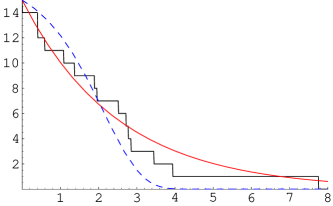
Figure 1: $N(>E)$ as a function of $\log E/E_{\rm min}$. The black stepwise line is the function $N(>E)$ generated by the simulation. The continuous (red) line is eq. (4) with $k=0.66$ (hence $\gamma=1.66$), while the dotted (blue) line is a fit to eq. (5). Both curves are normalized so that $N(>E)=15$ at $E=E_{\rm min}$.

The spectrum of accidentals must be measured experimentally and, if it drops exponentially, a strategy to search for GW bursters is to perform the data analysis with a very high cut on the energy of the events, since real signals drop only as a power-law. If the detectors are so clean that with these cuts the number of total expected accidentals, computed from the shifting algorithm mentioned above, becomes much smaller than one, then even the presence of a few coincidences could be significant.

When we look for high-energy events we can relax other cuts. For instance, in the analysis of data from resonant bars, presently are taken into consideration only data stretches where the average effective temperature of the bar is smaller than a given value, say 6 mK. This is very reasonable when, as in Ref. ROG01 , we look for events that depose in the bar more than O(30) mK (which corresponds to a dimensionless GW amplitude $h=O(10^{-18})$ for a burst with a duration $\sim 1$ ms). However, if we restrict to events of hundreds of mK, the fact that the detector temperature was 6 or 10 mK has little importance, and we can relax this condition. This has the consequence that the stretches of useful data become significantly longer. Furthermore, the orientation of the detector with respect to a source changes with sidereal time because of the Earth rotation. Low-energy events, which are close to the detection threshold, can therefore be easily missed when the detector is not favorably oriented, while high-energy events are efficiently detected independently of sidereal time.

Waiting time distribution. The statistics of waiting times (the times between an event and the next) of both earthquakes and SGRs is very different from that of uncorrelated events. Earthquakes, SGRs and other phenomena related to self-organized criticality have periods of intense bursting activity, during which the events arrive in bunches or there is a large event followed by showers of smaller events; these intense periods are then followed by long, and sometime extremely long, periods of quiescence. To quantify this property, it is convenient to introduce the quantity $n(<\tau;N)$, defined as the number of events with waiting time smaller than $\tau$, when the total number of events detected is $N$. Like $N(>E)$ defined in eq. (3), this is an integrated quantity, in order to circumvent the same binning problem discussed for the energy spectrum. Observe that the waiting time between one event and the next depends strongly on the resolution that we have for detecting the events: with a very good resolution we will find many small events which otherwise would go undetected, and correspondingly the waiting times will be shorter. Therefore, when we compare the waiting time statistics of different phenomena like SGR, earthquakes or GW bursts, we must always perform the comparison at a fixed value of the total number $N$ of events detected, taking the $N$ most energetic events from each sample. We normalize $n(<\tau;N)$ to the total number of events $N$, defining $w(\tau;N)=(1/N)\,n(<\tau;N)$, so $0\leq w(\tau;N)\leq 1$. We also normalize $\tau$ to the total observation time, so $0\leq\tau\leq 1$. A remarkable result is that SGR and earthquakes have the same waiting time distribution Che . With the very large statistical sample from SGR1900+14 mentioned above, it has been shown that their waiting time distributions are compatible with log-normal functions Gog .

For GW detection, unfortunately, we will rather be in the opposite limit of very low number of events. Therefore we now investigate whether the waiting time distribution for SGR1900+14, taking for definiteness only the 9 more energetic events detected in a six months period in 1998, when the source was very active, can be distinguished from the distribution of uncorrelated events.

The waiting time statistics of uncorrelated events can easily be computed analytically: the probability distribution $p(\tau;N)d\tau$ for having a waiting time between $\tau$ and $\tau+d\tau$ when we have a total of $N$ events (normalized so that $\int_{0}^{1}d\tau p(\tau;N)=1$) is a binomial distribution

$$p(\tau;N)=N(1-\tau)^{N-1}\,.$$ (6)

We also checked this result numerically generating random arrival times. Therefore for randomly distributed arrival times

$$w_{\rm ran}(\tau;N)=\int_{0}^{\tau}d\tau^{\prime}p(\tau^{\prime};N)=1-(1-\tau)^{N}\,.$$ (7)

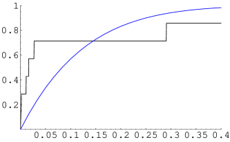
Figure 2: $w(\tau)$ against $\tau$, for the 9 more energetic events from SGR1900+14 during a 6 months period in 1998 (black stepwise curve) and $w_{\rm ran}(\tau;N)$ for $N=9$ (blue continuous line).

In Fig. 2 we show the experimental distribution for the 9 most energetic events from SGR1900+14 Apt , and we compare it with the function $w_{\rm ran}(\tau;N)$ for $N=9$. Even with the uncertainties due the use of such a limited sample, we see that the curve for random events is not compatible with the experimental data. In particular, two features stand out in the data. First, at very low $\tau$, the experimental values of $w(\tau)$ are much higher that the prediction for random events. For instance the fraction of events with waiting times smaller than $\tau\simeq 0.03$ (recall that the total observation time has been normalized to one, so this means waiting times smaller than $3\%$ of the total observation time) is over $70\%$ of the total, while in a random distribution it should be about $20\%$. Physically, this reflects the existence of periods of very intense activity, when the events arrive in bunches. Second, the experimental curve crosses $w_{\rm ran}(\tau;N)$ and then reaches the value $w=1$ at $\tau=1$ (fixed by normalization) staying below $w_{\rm ran}(\tau;N)$. Physically, this reflects the existence of long periods of quiescence.

This suggest that, even with a rather limited sample, the waiting time distribution expected for GW bursters is so peculiar that it can be distinguished from that due to random events. A different question is whether accidental coincidences in GW detectors follow the waiting time distribution of random events. In general, a certain amount of clustering must be expected because, for various reasons, in certain periods the detectors can be more noisy. However, this is an issue that can be studied experimentally. The distribution of accidental coincidences in two detectors, obtained from the shifting algorithm, can be fully characterized, and its waiting time statistics can be compared to that expected for uncorrelated events and for SGRs.

As discussed at length in Ref. CDM , for a source emitting repeatedly GW bursts another useful tool is a sidereal time analysis, since the events will be detected with higher efficiency when the detector is favorably oriented with respect to this source. This effect will be more important for low-energy events, i.e. for events close to the detector threshold, while the number of detected high-energy events is largely insensitive to the detector orientation. The sidereal time analysis is therefore complementary to the study of the waiting time and energy distributions discussed in this paper.

Finally, all mechanisms that generate GW bursters are likely to produce x- or $\gamma$-rays and therefore it might be possible a simultaneous detection of photons and GWs.

Acknowledgments. We are grateful to Eugenio Coccia for many useful discussions. Our work is partially supported by the Fond National Suisse.

References

- (1) P. Astone et al., Class. Quant. Grav. 19 (2002) 5449.
- (2) B. Abbott et al., Phys. Rev. D69 (2004) 102001
- (3) E. Coccia, F. Dubath and M. Maggiore, Phys. Rev. D70 (2004) 084010, arXiv:gr-qc/0405047.
- (4) S.L. Shapiro and S.A. Teukolsky, “Black Holes, White Dwarfs and Neutron Stars”, Wiley 1983. p. 12.
- (5) R. C. Duncan and C. Thompson, Astrophys. J. 392 (1992) L9.
- (6) C. Thompson and R. C. Duncan, Astrophys. J. 408 (1993) 194; ibid. 473 (1996) 322; Mon. Not. R. Astron. Soc. 275 (1995) 255.
- (7) J. A. de Freitas Pacheco, Astron. Astrophys. 336 (1998) 397.
- (8) K. Ioka, Mon. Not. R. Astron. Soc. 327 (2001) 639.
- (9) M. Ruderman, Nature 223 (1969) 597.
- (10) R. Smolukowski and D. Welch, Phys. Rev. Lett. 24 (1970) 1191.
- (11) A. Drago, G. Pagliara and Z. Berezhiani, arXiv:gr-qc/0405145.
- (12) G. F. Marranghello, C. A. Z. Vasconcellos and J. A. de Freitas Pacheco, Phys. Rev. D 66 (2002) 064027.
- (13) P. Bak, How Nature Works, Oxford Univ. Press, 1997.
- (14) B. Gutenberg and C. F. Richter, Bull. Seis. Soc. Am. 46 (1956) 105.
- (15) B. Cheng et al. Nature 382 (1995) 518.
- (16) P. Woods et al., Astrophys. J. 519 (1999) L139.
- (17) E. Gögüs et al., Astrophys. J. 532 (2000) L121.
- (18) K. Hurley et al., Nature 397 (1999) 41.
- (19) J. I. Katz, J. Geophys. Res. 91 (1986) 10412.
- (20) R. L. Aptekar et al., arXiv:astro-ph/0004402.