Inflation has the potential to seed the galactic magnetic fields observed today. However, there is an obstacle to the amplification of the quantum fluctuations of the electromagnetic field during inflation: namely the conformal invariance of electromagnetic theory on a conformally flat underlying geometry. As the existence of a preferred minimal length breaks the conformal invariance of the background geometry, it is plausible that this effect could induce electromagnetic field amplification. We show that this scenario is equivalent to endowing the photon with a large negative mass during inflation. This effective mass is negligibly small in a radiation and matter dominated universe. Depending on the value of the free parameter in the theory, we show that the seed required by the dynamo mechanism can be generated. We also show that this mechanism can produce the requisite galactic magnetic field without resorting to a dynamo mechanism.

1 Introduction

Cosmic magnetic fields are ubiquitous at all large intragalactic scales. It is a well-known observational fact that our galaxy and many other spiral galaxies are endowed with coherent magnetic fields of $\mu$G (microgauss) strength [1, 2, 3, 4, 5], having approximately the same energy density as the cosmic microwave background radiation (CMBR). There is also evidence for larger magnetic fields of similar strength within clusters [6, 7]. The presence of magnetic fields at larger scales has also been confirmed [8, 9]. These magnetic fields play an important role in various astrophysical processes, such as the confinement of cosmic rays and the transfer of angular momentum away from protostellar clouds so that they can collapse and become stars. Magnetic fields are also present in the intracluster gas of rich clusters of galaxies, in quasistellar objects (QSO’s) and in active galactic nuclei. They may influence the formation process of large-scale structure [10, 11].

It is widely believed that galactic magnetic fields are amplified and sustained by a dynamo mechanism [3, 4, 5, 12, 13, 14], in which the cyclonic turbulent motion of ionized gas combined with the differential rotation of the galaxy exponentially amplifies a “seed” magnetic field. This continues until the backreaction of the motion of the plasma offsets the growth of the field, stabilizing it to dynamical equipartition strength. However, while the dynamo mechanism provides an amplification mechanism, it does not explain the origin of galactic magnetic fields, and requires a “coherent” seed magnetic field for it to be effective. Indeed, it has been shown that seed magnetic fields that are too incoherent may undermine the action of the dynamo [15]. Most dynamo scenarios require a minimum coherence length equal to the dimension of the largest turbulent eddy, usually around $\sim 100$ pc. If the mechanism has functioned over the whole age of the galaxy($\sim$ 10G yr) a seed field of $10^{-19}$G is required. If recent observations are correct and the universe is dominated by a dark-energy density component [16, 17], then galaxies are older than previously thought and the seed magnetic field may be as low as $B_{seed}\sim{10}^{-30}$G [18].

A contrasting view is that the primeval magnetic flux trapped in the gas that collapsed to form the galaxy is responsible for the existence of galactic magnetic fields. This hypothesis also requires the existence of a seed magnetic field, one that is as great as the field observed today [19, 20]. Several scenarios have been suggested for creation of the required seed magnetic field, the most important of which involve battery [15] or vorticity [21] effects. The battery mechanism requires a large-scale misalignment of density and pressure gradients usually related to active galactic nuclei (AGN) or starburst activity. Therefore, it is difficult to realize in the majority of galaxies. The vorticity mechanism is based on the relative motions of photons and electrons induced by vorticity that was present before decoupling. Of course this mechanism assumes the existence of primeval vorticity. In addition, large-scale vortical motions can be effective only if ionization of the plasma is considerable, which does not occur at the galaxy-formation epoch.

Throughout most of the history of the universe the average time $\tau$ between particle interactions has been much smaller than the expansion time scale, $\tau\ll t_{Hubble}$ . Consequently the universe has been a good conductor [22], and any primeval cosmic magnetic field would have evolved in a manner that preserved magnetic flux: $Ba^{2}\sim$ constant, where $a$ is the scale factor. Hence the dimensionless ratio $r=B^{2}/\left(8\pi\rho_{\gamma}\right)$ is almost constant and provides a convenient measure of magnetic field strength. If there had been a pregalactic cosmic magnetic field that collapsed with the gas that formed the galaxy, its strength must have increased as $\mathbf{[\rho}_{gal}\mathbf{/\rho}_{tot}(t)]^{2/3}$, where $\rho_{tot}(t)$ is the average cosmic mass density at time $t$. As $\rho_{tot}\propto a^{-3}$ and $\rho_{gal}/\rho_{tot}=10^{6}$ today ($t_{0}=0$), it follows that the strength of the magnetic field at the time of formation $t_{form.}$ must have been $10^{4}[a(t_{form.})/a(t_{0})]^{2}B_{cosmic}$ or $B_{gal.}\simeq 3r^{1/2}10^{-2}$G. This yields $r\simeq 10^{-34}$ for initiating the galactic dynamo, or alternatively $r\simeq 10^{-8}$ for seeding the galactic magnetic field itself while avoiding the necessity of a galactic dynamo. If the existence of dark energy in the universe is confirmed, the minimum $r$ required to seed the dynamo mechanism reduces to $10^{-56}$.

Inflation offers the hope of furnishing a mechanism for kinematically and dynamically producing the seed for cosmic magnetic fields. It provides the kinematic means for producing long-wave-length effects at very early times through microphysical processes operating on scales less than the Hubble radius. Since an electromagnetic wave with $\lambda_{phys}\geq H^{-1}$ has the appearance of static $\mathbf{E}$ and $\mathbf{B}$ fields, very long wavelength photons ($\lambda_{phys}\gg H^{-1}$) can lead to large-scale magnetic fields (which then become supported by currents). Of course the electric field generated during the inflationary stage not only is not amplified, but is actually damped down due to the large conductivity of the primeval plasma. Another reason inflation is considered to be a prime candidate for field amplification is the fact that during inflation the universe is devoid of charged particles. Hence, the magnetic flux is not necessarily conserved and $r$ can increase. Furthermore, inflation can superadiabatically amplify the energy density($\simeq kd\rho/dk$) of the minimally coupled field [23]. Then the energy density decays as $a^{-2}$, rather than the usual result $a^{-4}$(“adiabatic result”).

However the conformal flatness of the Robertston-Walker metric prevents the background gravitational field from producing particles, provided the underlying matter theory is conformally invariant. A pure U(1) gauge theory with the standard lagrangian $\mathcal{L}=-\frac{1}{4}F_{\mu\nu}F^{\mu\nu}$ is conformally invariant, from which it follows that $\rho_{B}\propto B^{2}$ always decreases as $a^{-4}$. During the inflationary epoch, the total energy density in the universe is dominated by vacuum energy and therefore the energy density in any magnetic field during inflation is significantly suppressed. In fact it can be shown that $r=10^{-104}\lambda_{Mpc}$ [22], where $\lambda_{Mpc}\equiv\lambda/1Mpc$.

Several proposals have been given to break the conformal invariance of the theory: (i) coupling the electromagnetic field to a non-conformally-covariant charged field [24], (ii) coupling the electromagnetic field to gravity via either gauge non-invariant terms such as $RA_{\mu}A^{\mu}$, $R_{\mu\nu}A^{\mu}A^{\nu}$ or gauge invariant ones like $R_{\mu\nu\lambda\kappa}F^{\mu\nu}F^{\lambda\kappa}/m^{2}$, $R_{\mu\nu}F^{\mu\kappa}F_{\kappa}{}^{\nu}/m^{2}$ or $RF^{\mu\nu}F_{\mu\nu}/m^{2}$ [22], (iii) invoking effects due to the quantum conformal anomaly [25, 26], (iv) creating primordial magnetic fields at either the QCD transition epoch [27] or the electroweak transition [28], (v) breaking conformal invariance via nonzero vacuum expectation values of flat directions in minimally supersymmetric standard models (MSSM) [29].

Attempts to realize the first possibility were carried out by coupling the electromagnetic field to the scalar field $\Phi$ responsible for inflation via a term $\propto e^{\Phi}F^{\mu\nu}F_{\mu\nu}$ [24]. This investigation showed that in the exponential potential for the inflaton

$$V(\Phi)=(\frac{6-q}{3})\frac{16\pi}{{m_{pl}}^{2}}\rho_{b\Phi}^{0}e^{(-\sqrt{\frac{q}{2}}(\Phi-\Phi_{0}))},$$ (1)

it is possible to generate an intergalactic magnetic field whose present strength (depending on values of parameters of the model) lies between $10^{-65}$ to $10^{-10}$ on a scale of $1/1000$ that of the Hubble scale. In (1) $m_{Pl}$ is the planck mass, $\Phi^{0}$ is the value of the scalar field and $\rho_{b\Phi}^{0}$ is the homogeneous scalar field energy density when the scale factor is $a_{0}$. Thus in this scenario one can have the desired galactic magnetic field by resorting to the dynamo mechanism.

Considering next possibility (ii), if we add gauge non-invariant terms to the action, the $U(1)$ gauge invariance will be broken. To avoid the phenomenological disasters this can cause one can endow the photon with a mass squared of the order of $H^{2}$ (well below present limits of detectability). It has been shown [22] that such a term can create primeval fields with strength as large as $r\sim 10^{-8}$ .

Gauge invariant modifications to the action have much better theoretical motivation. For example, all $RF^{2}$ terms can be obtained by calculating the effective Lagrangian for QED in curved space-time to one loop order [30]. At early times, when $R^{1/2}\sim H\sim\rho_{tot}^{1/2}/m_{pl}\gg 10^{-11}m_{pl}$, these terms govern the behavior of the electromagnetic field. However at later times, when $R^{1/2}\ll 10^{-11}m_{pl}$, they are negligible compared to the standard $-\frac{1}{4}F^{2}$ term. In a power-law inflationary background the amplitude of large-scale fields is not large enough to be astrophysically interesting [22].

The third possibility has proven to be promising for gauge theories with large groups and a greater number of bosons than fermions. In such theories, it has been shown that this mechanism for breaking conformal invariance in quantum electrodynamics can create a sufficient amount of primordial magnetic field [25]. However, in the simplest version of the grand unified $SU(5)$ model with three generations of fermions the magnetic field produced is below the requirement of the dynamo mechanism.

Phase transitions at different cosmological epochs (grand unification, the electroweak transition [28] or the quark confinement epoch [27]) have also been considered. However, since the generating mechanisms are causal, the coherence of the created magnetic field cannot be larger than the particle horizon at the time of the phase transition. Because all the above transitions occurred very early in the universe’s history, the comoving size of the horizon is rather small. The best case is the QCD transition, for which the horizon corresponds to $\sim$ 1 a.u. Consequently the real magnetic fields generated lack sufficient coherence.

The MSSM flat directions, made up of gauge invariant combinations of squarks and sleptons, acquire non-vanishing vacuum expectation values (vev) during inflation. These flat directions endow the standard model gauge fields with mass and break the conformal invariance. The quantum fluctuations of these flat directions, in contrast to the their classical vevs, induce fluctuations in the gauge degrees of the freedom that cannot be gauged away. The gauge field fluctuations that are stretched outside the horizon during inflation, provide us with a seed (hyper)magnetic field after they re-enter the horizon. They give rise to $U(1)_{em}$ magnetic field with strength of $10^{-30}$ G, as required by the dynamo mechanism [29].

Here we consider an alternative mechanism that is based on a hypothesis of a minimal fundamental length scale. Minimal length breaks conformal invariance and so it might be expected that primordial magnetic fields can be produced during inflation. One suggestion [31] for implementing minimal length into the inflationary scenario in the context of trans-planckian physics [32] is based on the hypothesis of a generalized uncertainty principle:

$$\Delta x\Delta p\geq\frac{1}{2}\left(1+\beta~{}(\Delta p)^{2}\right),$$ (2)

where $\sqrt{\beta}$ is the ultraviolet cutoff on the order of the Planck or string length. In this paper we employ this formalism to implement minimal length into the action of electrodynamics. This translates into a UV cutoff which, once implemented, has the sole effect of modifying the evolution of the electromagnetic field. As we will demonstrate, the formalism is not able to create a squeezing effect for the electromagnetic field. Therefore the energy density of the electromagnetic field attenuates adiabatically, $\rho_{B}\propto a^{-4}$.

However, it has recently been shown [33] that terms in the action that are total time derivatives are not invariant under the influence of the minimal length hypothesis [31]. Consequently such terms contribute to the equations of motion of the matter fields. We consider in this paper an example of a total time derivative that, under the influence of the UV cutoff, causes the photon to gain a large negative mass during inflation. This effect goes to zero at the end of inflation and so such a mass is undetectable today. We shall show that this approach is successful in providing the dynamo mechanism with sufficient primordial seed magnetic field. Even in absence of the dynamo mechanism, one can adjust a free parameter in the action to account for the observed magnetic field of galaxies today.

2 Cutoff Breaking of Conformal Invariance

The existence of a preferred minimal length breaks the conformal invariance of the background geometry. Here we will examine the effect of this conformal breaking on the evolution of electromagnetic fields.

We introduce a fundamental length (i.e. the presence of a cut-off) in the inflationary scenario via generalization of the quantum mechanical commutation relation [31]

$$[\mathbf{X},\mathbf{P}]=i\longrightarrow[\mathbf{X},\mathbf{P}]=i\left(f\left(\beta\right)\mathbf{1}+g(\beta)\mathbf{P}^{i}\mathbf{P}^{j}\right)$$ (3)

where $f\left(\beta\right),g\left(\beta\right)$ are functions such that $f\left(0\right)=1$ and $g\left(0\right)=0$; their actual form is determined by other criteria that we shall discuss below. This generalization significantly modifies transplanckian physics, whose effects are then manifest in the CMBR. Here we employ the above formalism to find the effect this cutoff has on the evolution of magnetic fields.

We begin with the action of electromagnetism in an expanding curved background

$$S=-\int\frac{1}{4}\sqrt{-g}g^{\mu\nu}g^{\alpha\beta}F_{\mu\alpha}F_{\nu\beta}d^{3}\mathbf{y}d\eta$$ (4)

where the $y^{i}$’s are comoving spatial coordinates related to the proper ones by $x^{i}=a(\eta)y^{i}$ and $\eta$ is the conformal time. Assuming that the background is flat Friedmann Robertson Walker, with the metric

$$ds^{2}=\left\{\begin{array}[]{ll}-dt^{2}+a^{2}(t)\sum\limits_{i=1}^{i=3}{dy^{i}}^{2}&\\ a^{2}(\eta)(-d\eta^{2}+\sum\limits_{i=1}^{i=3}{dy^{i}}^{2}),&\end{array}\right.$$ (5)

one can write down the action in the following form:

$$S=\frac{1}{4}\int[2F_{oi}F_{oi}-F_{ik}F_{ik}]d^{3}\mathbf{y}d\eta$$ (6)

Roman indices $i$ and $k$ run from 1 to 3 and repeated indices are summed over. The disappearance of the scale factor $a(\eta)$ is a consequence of the conformal invariance of electromagnetism. By imposing the radiation gauge $A_{0}=\partial_{i}A_{i}=0$, the above action can be rewritten in the following form

$$S=\frac{1}{2}\int[(\partial_{0}\mathbf{A})^{2}-(\mathbf{\nabla}\times\mathbf{A})^{2}]d^{3}\mathbf{y}d\eta.$$ (7)

in terms of the electromagnetic potential $A_{i}$. This action is the familiar electrodynamic action,

$$S=\frac{1}{2}\int(\mathbf{E}^{2}-\mathbf{B}^{2})d^{3}\mathbf{y}d\eta,$$ (8)

written in radiation gauge.

The most general form of the modified commuation relation (3) that breaks Lorentz invariance (see also [34]) while preserving the translational and rotational symmetry takes the following form [31, 35]

$$[\mathbf{X}^{i},\mathbf{P}^{j}]=i\left(\frac{2\beta p^{2}}{\sqrt{1+4\beta p^{2}}-1}\delta^{ij}+2\beta\mathbf{P}^{i}\mathbf{P}^{j}\right)$$ (9)

to first order in the parameter $\beta$. Here $p$ is the physical momentum. We still assume that $[\mathbf{X}^{i},\mathbf{X}^{j}]=[\mathbf{P}^{i},\mathbf{P}^{j}]=0$. To impose this modified commuation relation, we rewrite the action using proper spatial coordinates $x=a(\eta)y$ in the form:

$$S=\frac{1}{2}\int\frac{d\eta d^{3}\mathbf{x}}{2a^{3}}\left\{\left(\left[\partial_{\eta}+\frac{a^{\prime}}{a}\partial_{x^{i}}x^{i}-\frac{3a^{\prime}}{a}\right]\mathbf{A}\right)^{2}-a^{2}\left(\nabla\times\mathbf{A}\right)^{2}\right\}$$ (10)

We can identify $-i\partial_{x^{i}}$ as the momentum operator, $\mathbf{P}^{i}$ , and $x^{i}$ as the position operator, $\mathbf{X}^{i}$. We can cast the action (41) to a simpler form:

$$S=\int\frac{d\eta}{2a^{3}}\left\{\big{(}\mathbf{A},B^{{\dagger}}(\eta)B(\eta)\mathbf{A})+a^{2}(\mathbf{P}\times\mathbf{A}\big{)}^{2}\right\},$$ (11)

where we have consolidated $(\partial_{\eta}+i\frac{a^{\prime}}{a}\sum_{i=1}^{3}\mathbf{P}^{i}\mathbf{X}^{i}-3\frac{a^{\prime}}{a})$ into a new operator $B(\eta)$. Since $\partial_{i}A^{i}=0$, it means that $(\mathbf{P}\times\mathbf{A})^{2}=\mathbf{P}^{2}\mathbf{A}^{2}$. A suitable vectorial Hilbert space representation of the new commutation relation can be defined by using auxiliary variables $\rho^{l}$:

$$\mathbf{X}^{l}\mathbf{A}(\rho)=i\partial_{\rho^{l}}\mathbf{A}(\rho)$$ (12)

$$\mathbf{P}^{l}\mathbf{A}(\rho)=\frac{\rho^{l}}{1-\beta\rho^{2}}\mathbf{A}(\rho)$$ (13)

$$(A_{i}(\rho),A_{j}^{\prime}(\rho))=\int_{\rho^{2}<\beta^{-1}}d^{3}\rho A_{i}^{\ast}(\rho)A_{j}^{\prime}(\rho)$$ (14)

Recall that the usual quantum mechanical commutation relation, $[X^{i},P^{j}]=i\delta^{ij}$ is defined on a Hilbert space with the following representation

$$\mathbf{X}^{l}\mathbf{A}(\rho)=x^{l}\mathbf{A}(x)$$ (15)

$$\mathbf{P}^{l}\mathbf{A}(\rho)=-i\partial_{x^{l}}\mathbf{A}(x)$$ (16)

$$(A_{i}(x),A_{j}^{\prime}(x))=\int d^{3}\mathbf{x}A_{i}^{\ast}(x)A_{j}^{\prime}(x)$$ (17)

Ultimately the action takes the following form:

$$S=\int d\eta\int_{\rho^{2}<\beta^{-1}}d^{3}\rho\frac{1}{2a^{3}}\left\{|(\partial_{\eta}-\frac{a^{\prime}}{a}\frac{\rho^{i}}{1-\beta\rho^{2}}\partial_{\rho^{i}}-\frac{3a^{\prime}}{a})\mathbf{A}|^{2}-\frac{a^{2}\rho^{2}|\mathbf{A}|^{2}}{(1-\beta\rho^{2})^{2}}\right\}$$ (18)

The presence of $\rho$ derivatives means that the $\rho$ modes are coupled. However we can find new variables ($\tilde{\eta},\tilde{k}$)

$$\tilde{\eta} = \eta,$$

$$\tilde{k}^{i} = a\rho^{i}e^{(-\beta\rho^{2}/2)}$$ (19)

where the $\tilde{k}$ modes decouple because

$$\partial_{\eta}-\frac{a^{\prime}}{a}\frac{\rho^{i}}{1-\beta\rho^{2}}\partial_{\rho^{i}}=\partial_{\tilde{\eta}}$$ (20)

We will use the common index notation $\bar{A}_{\tilde{k}}$ for those decoupling modes. The $\tilde{k}$ modes coincide with the usual comoving modes on large scales, i.e., only for small $\rho^{2}$. This means that the comoving k modes that are obtained by scaling, $k^{i}=ap^{i}$, decouple at large distances and couple at small distances. The action now takes the form

$$S=\int d\tilde{\eta}\int_{\tilde{k}<a^{2}/e\beta}d^{3}\tilde{k}\mathcal{L}$$ (21)

where

$$\mathcal{L=}\frac{1}{2}\nu\left\{{\left|\left(\partial_{\eta}-3\frac{a^{\prime}}{a}\right)\mathbf{\bar{A}}_{\tilde{k}}\right|}^{2}-\mu\left|\mathbf{\bar{A}}_{\tilde{k}}\right|^{2}\right\}$$

We have defined $\mu$ and $\nu$ as

$$\mu(\eta,\rho)\equiv\frac{a^{2}\rho^{2}}{(1-\beta\rho^{2})^{2}}$$ (22)

$$\nu(\eta,\rho)\equiv\frac{e^{3\beta\rho^{2}/2}}{a^{6}(1-\beta\rho^{2})}$$ (23)

It is convenient to express these functions in terms of the Lambert $W$ function (defined so that $W(x)e^{W(x)}=x$ [36])

$$\mu(\eta,\tilde{k})=-\frac{a^{2}}{\beta}\frac{W(\zeta)}{(1+W(\zeta))^{2}}$$ (24)

$$\nu(\eta,\tilde{k})=\frac{e^{-3W(\zeta)/2}}{a^{6}(1+W(\zeta))}$$ (25)

where $\zeta=-\beta\tilde{k}^{2}/a^{2}$. The equation of motion for the action (21) is:

$$\bar{\mathbf{A}}_{\tilde{k}}^{\prime\prime}+\frac{\nu^{\prime}}{\nu}\bar{\mathbf{A}}_{\tilde{k}}^{\prime}+\bigg{(}\mu-3\frac{\nu^{\prime}}{\nu}(\frac{a^{\prime}}{a})-3\big{(}\frac{a^{\prime}}{a}\big{)}^{\prime}-9(\frac{a^{\prime}}{a})^{2}\bigg{)}\bar{\mathbf{A}}_{\tilde{k}}=0$$ (26)

The operations of Fourier transforming and of scaling from proper position coordinates do not commute [31]. Hence the field variable $\bar{\mathbf{A}}_{\tilde{k}}$ is different from that commonly employed in the literature, $\mathbf{A}_{\tilde{k}}$ by a factor of $a^{3}$:

$$\bar{\mathbf{A}}_{\tilde{k}}=a^{3}{\mathbf{A}}_{\tilde{k}}$$ (27)

Taking into account eq.(27) and introducing a new variable $\theta:=a^{6}\nu$, we obtain

$$\mathbf{A}_{\tilde{k}}^{\prime\prime}+\frac{\theta^{\prime}}{\theta}\mathbf{A}_{\tilde{k}}^{\prime}+\mu\mathbf{A}_{\tilde{k}}=0;$$ (28)

as the equation of motion for scalar perturbations in presence of a minimal length cutoff.

The solutions to equation (28) are constrained by the Wronskian condition which follows from the canonical commutation relation between $\mathbf{A}_{\tilde{k}}$ and its conjugate momentum, $\mathbf{\Pi}_{\tilde{k}}=\theta\mathbf{A}_{\tilde{k}}^{\prime}$

$$[A_{\tilde{k}}^{i},\Pi_{\tilde{k}^{\prime}}^{j}]=i\delta^{ij}\delta^{3}(\tilde{k}-\tilde{k}^{\prime})$$ (29)

or equivalently

$$A_{\tilde{k}}^{i}A_{\tilde{k}}^{{}^{\prime}j\ast}-A_{\tilde{k}}^{i\ast}A_{\tilde{k}}^{{}^{\prime}j}=i\theta^{-1}\delta^{ij}$$ (30)

During the de Sitter phase, $a=-1/H\eta$ and so $\zeta=-\beta H^{2}\tilde{k}^{2}\eta^{2}$. $\sigma=\sqrt{\beta}H$ is the ratio of the cutoff to the Hubble parameter during inflation. The factors $\mu$ and $\theta^{\prime}/\theta$ have the following expansions in the limit in which the mode is outside the horizon ($\tilde{k}\eta\ll 1$):

$$\mu(\eta,\tilde{k}) = \tilde{k}^{2}+3\beta^{2}H^{2}\tilde{k}^{4}\eta^{2}+\cdots$$ (31)

$$\frac{\theta^{\prime}(\eta,\tilde{k})}{\theta(\eta,\tilde{k})} = 5\beta H^{2}\tilde{k}^{2}\eta+12\beta^{2}H^{4}\tilde{k}^{4}\eta^{3}+\cdots$$ (32)

In that regime, the modes satisfy the following equation:

$$\mathbf{A}_{\tilde{k}}^{\prime\prime}+\tilde{k}^{2}\mathbf{A}_{\tilde{k}}=0$$ (33)

Thus $\mathbf{A}_{\tilde{k}}\propto e^{i\tilde{k}\eta}$ and $\mathbf{B}_{i}=\epsilon_{ilm}F_{lm}/a^{2}$ where $F_{lm}=\partial_{l}A_{m}-\partial_{m}A_{l}$. As a result $\rho_{B}$ varies like $a^{-4}$, which is the adiabatic result.

Superficially this mechanism is unable to amplify the cosmic magnetic fields. However it has been shown that this method of implementing the cut-off in the action has an ambiguity: total time derivatives no longer reduce to pure boundary terms [33]. In continuous space-time, the presence of such a boundary term does not affect the evolution of the electromagnetic potential. However the operator $\partial_{\eta}$ that acts on the electromagnetic potential inside the total time derivative transforms to $B(\eta)$ in the proper spatial coordinates. Since the modification of the commutation relation between $X^{i}$ and $P^{j}$ affects how this operator acts upon $A_{\mu}$, this procedure of implementing minimal length will not keep such total time derivatives invariant.

Fortunately another option is available. It can be shown that any boundary term in physical space transforms to a non-boundary term in momentum space in the following manner:

$$\int(f(a,A))^{\prime}d^{3}\mathbf{y}d\eta\rightarrow\int\theta(\eta,\tilde{k})(f(a,A_{\tilde{k}}))^{\prime}d^{3}\tilde{k}d\eta$$ (34)

and so it is possible that they may contribute to the equation of motion in such a way that the above behavior of the magnetic field is modified. Since we wish to break the conformal invariance, we endow the photon with a mass term [37, 38]. This implies that $f(a,A)=g(a,a^{\prime},\ldots)A^{\mu}A_{\mu}$. However we also do not want to modify the behavior of the photon in the well-understood part of the history of the universe, namely the radiation and matter dominated eras. Since during these eras the scale factor respectively behaves as $\eta$ and $\eta^{2}$, we assume that $g(a)\propto a^{\prime\prime\prime}$. So far the proposed boundary term adds to Eq.(33) a term $\propto-\frac{a^{\prime\prime\prime}\theta^{\prime}}{a^{2}\theta}\mathbf{A}_{\tilde{k}}$ which looks like $\mathbf{A}_{\tilde{k}}/\eta$ as the mode crosses outside the horizon. Recalling the equation of motion for scalar fluctuations, $u_{k}$ (see for e.g. [33])

$$u_{k}+(k^{2}-\frac{z^{\prime\prime}}{z})u_{k}=0,$$ (35)

the term that creates the amplification is $z^{\prime\prime}u_{k}/z$ which behaves like $u_{k}/\eta^{2}$ as the mode is far outside the horizon. Hence we multiply the previous term with another factor of $a$ to produce the desired behavior.

Summarizing, the proposed boundary term is:

$$\triangle S=\frac{1}{M_{1}^{2}}\int(A^{\mu}A_{\mu}a^{\prime\prime\prime}a)^{\prime}d^{3}\mathbf{y}d\eta$$ (36)

where $\mu$ runs over space-time indices $0\cdots 3$ and $M_{1}$ is an arbitrary constant with dimensions of mass whose presence keeps $\triangle S$ dimensionless. We can write this covariantly as

$$\triangle S=\frac{1}{M_{1}^{2}}\int\nabla_{\alpha}(\Xi\zeta^{\alpha})\sqrt{g}d^{3}\mathbf{y}d\eta$$

where $\Xi$ is the scalar function

$$\Xi=\frac{1}{3}\left(A^{\mu}A_{\mu}\right)\left(\nabla^{2}K-2\nabla^{\mu}\nabla^{\nu}K_{\mu\nu}\right)\sqrt{\zeta\cdot\zeta}$$

where $K_{\mu\nu}$ is the extrinsic curvature of the boundary surface whose normal is $n_{\mu}=\left(a(\eta),\vec{0}\right)$ and $\zeta^{\alpha}=\left(1,\vec{0}\right)$ is the conformal Killing vector of the spacetime. Also, one can express $a^{\prime\prime\prime}$ in the following form:

$$a^{\prime\prime\prime}=a^{4}H^{3}(1-2q+j)$$ (37)

where $q$ and $j$ are respectively the deceleration and jerk parameters defined as [39]

$$q = -\frac{\ddot{a}}{aH^{2}},$$ (38)

$$j = \frac{\dddot{a}}{aH^{3}},$$ (39)

where dot denotes differentiation with respect to the physical time. The presence of such a term modifies the propagator of the photon only during inflation. The vertices and propagator of the electron do not get modified at any time. Therefore, the amplitude for the diagrams that describe photon splitting [40], $\gamma\rightarrow n\gamma$, remain intact and hence abide with the current bounds that exist on photon splitting [41].

The equation of motion for $\mathbf{A}_{\tilde{k}}$ derived from the variation of the cutoff-modified action $S+\triangle S$ is

$$\mathbf{A}_{\tilde{k}}^{\prime\prime}+(\tilde{k}^{2}-\frac{1}{M_{1}^{2}}\frac{a^{\prime\prime\prime}\theta^{\prime}}{a\theta})\mathbf{A}_{\tilde{k}}=0,$$ (40)

During the de Sitter expansion, $a=-1/H\eta$. For modes outside the horizon, $\tilde{k}\eta\ll 1$, and eq.(40) reduces to

$$\mathbf{A}_{\tilde{k}}^{\prime\prime}-\frac{n}{\eta^{2}}\mathbf{A}_{\tilde{k}}=0$$ (41)

where $n=30\sigma^{2}\tilde{k}^{2}/M_{1}^{2}$. In this limit we have $|\mathbf{A}_{\tilde{k}}|\propto\eta^{m_{\pm}}$ where $m_{\pm}=\frac{1}{2}(1\pm\sqrt{1+4n})$. Here $\sigma=\sqrt{\beta}/H^{-1}$, where $\sqrt{\beta}$ is the minimal length associated with the ultraviolet cutoff and $H$ is the Hubble constant during inflation. The fastest growing solution during the de Sitter phase is proportional to $\eta^{p}$ or equivalently $a^{-p}$, where we set $p=m_{-}$ . Note that for $p=-1$ ($n=2$), $|\mathbf{A}_{\tilde{k}}|$ varies like $a$ and $\rho_{B}\propto a^{-2}$, which is the superadiabatic result. The evolution of electromagnetic waves during reheating and the matter-dominated (MD) era is described by the same equation as (40) with $a\propto\eta^{2}$, whereas in the radiation dominated (RD) epoch $a\propto\eta$. In these three epochs the effective mass of the photon vanishes and $\rho_{B}\propto a^{-4}$. During RD, MD, and reheating, the electromagnetic field behaves as it does in absence of the cut-off.

The ratio of the energy stored in the $k$-th mode of quantum fluctuations, $\rho_{B}(k)$, to the total energy density of the universe, $\rho_{tot}$, at first horizon-crossing, $a=a_{1}$, is approximately equal to $[M/m_{Pl}]^{4}$. Here $M^{4}$ is the vacuum energy density during inflation. Such a quantum fluctuation will be excited during the de Sitter expansion, ref.[42], and can be treated as a classical fluctuation in the electromagnetic field when it crosses outside the horizon. After horizon-crossing $\rho_{B}(k)$ varies as $a^{-2(p+2)}$ while the total energy density of the universe remains constant, $\rho_{tot}\propto M^{4}$. Since the extra term added to the equation of motion is zero during reheating, in the MD and RD epochs the stored energy density in the $k$-th mode magnetic fluctuation attenuates adiabatically, $\rho_{B}\propto a^{-4}$. In reheating and the MD era, the energy density of the universe decreases as $a^{-3}$ whereas in the RD epoch the total energy density of the universe diminishes as $a^{-4}$. Therefore the invariant ratio, $\rho_{B}(k)/\rho_{\gamma}$ on the scale $\lambda$ is:

$$r\simeq e^{-2N(\lambda)(p+2)}\bigg{[}\frac{M}{m_{Pl}}\bigg{]}^{8/3}\bigg{[}\frac{T_{RH}}{m_{Pl}}\bigg{]}^{4/3},$$ (42)

where $N(\lambda)$ is the number of e-folds the universe expands between the first horizon crossing of the comoving scale $\lambda$ and the end of inflation. It is given by the following equation [43]:

$$N(\lambda)=45+\ln\lambda_{Mpc}+\frac{2}{3}\ln(M_{14})+\frac{1}{3}\ln(T_{10})$$ (43)

and $M=M_{14}10^{14}$ GeV, $T_{RH}=T_{10}10^{10}$ GeV. Plugging this equation back into Eq.(42), one obtains

$$r\simeq(7\times 10^{25})^{-2(p+2)}\bigg{[}\frac{M}{m_{Pl}}\bigg{]}^{-4p/3}\bigg{[}\frac{T_{RH}}{m_{Pl}}\bigg{]}^{-2p/3}\lambda_{Mpc}^{-2(p+2)}$$ (44)

The above formula is correct regardless of whether horizon re-crossing takes place at the RD or MD eras. Note that we have normalized our comoving scales such that today physical scales are equal to comoving scales, i.e. $a_{today}=1$.

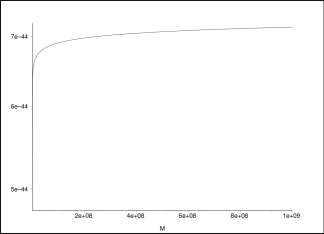
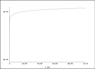
Figure 1: The left figure shows the dependence of $M_{1}$ on $M$, the energy scale of inflation. The right figure shows how $M_{1}$ varies as $T_{RH}$ changes. For all physically acceptable values of $M$ and $T_{RH}$, $M_{1}\sim 10^{-43}$GeV.

Two constraints on $M$ and $T_{RH}$ should hold in any viable scenario of inflation. First, to prevent the production of long-wavelength gravitons that distort the microwave background radiation beyond its upper limit of anisotropy, $M<10^{-2}m_{Pl}$ . Second, $M$ and $T_{RH}$ should be greater than $1$ GeV so that radiation domination takes place before nucleosynthesis.

To trigger the dynamo mechanism, there must be sufficient seed magnetic field at cosmologically interesting scales. This condition could be used to determine the value of $M_{1}$. Assuming that the required seed magnetic field has been substantial on galaxy-scales, $\lambda\sim 1$Mpc, one can obtain a relation between $M_{1}$ and other relevant parameters of the problem:

$$M_{1}\simeq\frac{1.6\times 10^{-38}\big{[}\ln(T_{RH}/m_{Pl})+3\ln b+2\ln(M/m_{Pl})\big{]}\sigma}{\bigg{(}\big{[}\ln r+4\ln b\big{]}\big{[}3\ln r+18\ln b+2\ln(T_{RH}/m_{Pl})+4\ln(M/m_{Pl})\big{]}\bigg{)}^{1/2}}Gev$$ (45)

where $b=7\times 10^{-25}$. If $M,T_{RH}$ and $\sigma$ are specified, one can obtain the corresponding values of $M_{1}$. In table 1, we have tabulated the results for different values of $M,T_{RH}$ corresponding to different scenarios of inflation and some values of $r$ required to initiate astrophysically interesting phenomena. As Fig.(1) and (2) show, for a fixed value of $\sigma$ and all physically relevant values of $M$ and $T_{RH}$, $M_{1}$ does not vary too much. For $\sigma\sim 10^{-5}$[33] we find $M_{1}\sim 10^{-43}$GeV. Since the coupling of the added term is proportional to $M_{1}^{-2}$, the smallness of $M_{1}$ indicates that the coupling of electromagnetic field to the curvature of the expanding background, due to the existence of minimal length, has been enormous during the inflationary era. However the coupling is extinguished in all other epochs due to the special form of the interaction.

Although we should await a unified theory to determine how gravity is coupled to the other fields of nature, this phenomenological scenario suggests that the enigmatic primordial magnetic fields might have their origin in the special characteristics of  space-time at high energies ( See also ref.[44] on how non-commutativity of the space-time might help us account for primeval magnetic fields).

$T_{RH}$(GeV)	$r|_{\lambda=1Mpc}$	$M_{1}\times 10^{43}$(GeV)
$10^{17}$	$10^{-8}$	$0.5639$
$10^{9}$	$10^{-8}$	$0.5103$
$10^{17}$	$10^{-34}$	$0.7311$
$10^{9}$	$10^{-34}$	$0.6638$
$10^{17}$	$10^{-56}$	$0.9819$
$10^{9}$	$10^{-56}$	$0.8973$

Table 1: Values for $M_{1}$ corresponding to different inflationary scenarios and different values of $r=(\rho_{B})/\rho_{\gamma}|_{1Mpc}$. Here $\sigma$ is assumed to be $10^{-5}$ and $M$ is held constant at $10^{17}$ GeV. $M_{1}$ does not vary significantly for all interesting values of $M,T_{RH}$ and $r$.

3 Conclusion

The origin of magnetic fields with $\mu$G strength that are observed on intragalactic scales remains an intriguing mystery. As the observed magnetic field is coherent on such cosmological scales, the first cosmological process one might think of as being able to produce such prevalent fields is inflation. However the conformal invariance of the electromagnetic field prohibits the quantum fluctuations of the electromagnetic field from squeezing and amplifying during inflation.

The existence of a minimal length breaks this conformal invariance. We have proposed a scenario based on this observation that can provide the requisite initial magnetic seed for the astrophysical dynamo mechanism. With a proper choice of the free parameter within the theory one can avoid the need for the dynamo mechanism.

The scenario is based on the observation that incorporating minimal length at the level of first quantization, as was done for the first time in [31], does not render total time derivatives invariant under the influence of minimal length. Therefore one can have actions that are equivalent at the continuous space-time level, but are distinct from one another once the presence of minimal length is introduced. We added a prototype for such a total time derivative term to the action of electromagnetism that respects the behavior of the photon throughout the history of the universe except for the inflationary era. During inflation this term induces a huge mass for the photon. We found that to match this model with observation we must tune the free parameter of the model, $M_{1}$, to be extremely small. Since $M_{1}^{-2}$ is proportional to the coupling of electromagnetism to the background geometry during inflationary epoch, the small size of $M_{1}$ is indicative of gravity and electromagnetism being strongly coupled at that time. We note that the numerical value of $M_{1}$ is approximately the inverse Hubble length, but we have found no deeper explanation for this coincidence at the level of the model presented here.

Of course it is conceivable that other gauge bosons of the standard model can inherit the same tachyonic instability that we have considered for the photon.  However all other gauge bosons are non-Abelian and so will experience screening effects that we expect will tend to dampen out this instability [45].  A detailed calculation of this effect remains an interesting subject for future study.

Of course the main drawback for this model is its arbitrariness in the choice of total time derivative. It would be really interesting if one were able to find candidates from existing models of fundamental physics. Our main goal here was that of demonstrating that specific characteristics of space-time at Planckian epochs can create observable phenomena in the universe at much later cosmological times.

References

- [1] Y. Sofue, M. Fujimoto and R. Wielebinski, Ann. Rev. Astron. Astrophys. 24, 459 (1986).
- [2] E. Asseo & H. Sol, 1987, Phys. Rep., 148, 307.
- [3] P. P. Kronberg, Rep. Prog. Phys. 57, 325 (1994).
- [4] R.Beck, A. Brandenburg, D. Moss, A. A. Sukhurov & D. Sokloff, Annu. Rev. Astron. Astrophys. 34, 155 (1996).
- [5] D. Grasso & H. R. Rubinstein, Phys. Rep. 348, 163 (2001).
- [6] R. A. Perely 1990, in IAU Symposium 140 Galactic and Intragalactic Magnetic Fields, edited by R. Beck, P. P. Kronberg & R. Wielebinski (Kluwar, Dordrecht, 1990), p. 463.
- [7] K.-T. Kim, P. C. Tribble and P. P. Kronberg, Astrophys. J. 379, 80 (1991).
- [8] G. Giovannini, K.-T. Kim, P. P. Kronberg & T. Venturi 1990, in IAU Symp. 140. Glactic and Intergalactic Magnetic Fields, ed. R. Beck, P. P. Kronbereg & Wielebinski (Dordrecht: Kluwar), 492.
- [9] J. P. Vallée, Astron. J. 99, 459 (1990).
- [10] K. Subramanian & D. Barrow, Phys. Rev. D57, 3264 (1998).
- [11] C. G. Tsagas & J. D. Barrow, Class. Quantum Grav. 15, 3523 (1998); J. P. Ostriker, C. Thompson & E. Witten, Phys. Lett. B180, 231 (1986).
- [12] E. N. Parker, Astrophys. J. 163, 255 (1971).
- [13] E. N. Parker, Cosmical magnetic fields (OUP, Oxford, 1979).
- [14] Y. B. Zel’dovich, A. A. Ruzmaikin & D. D. Sokollof, magnetic fields in Astrophysics (McGraw-Hill, New York, 1983).
- [15] R. M. Kulsrud & S. W. Anderson, Astrophys. J. 396, 606 (1992); R. M. Kulsrud & R. Cen, J. P. OStriker & D. Ryu, Astrophys. J. 480, 481 (1997); K. Subramanian, astro-ph/9707280.
- [16] Supernova Cosmology Project Collaboration, S. Perlmutter et. al., Astrophys. J. 517, 565 (1999); Nature (London) 391, 51 (1998); Supernova Search team Collaboration, A. G. Riess et. al. (Supernova Search team Collaboration), Astron. J. 116, 1009, (1998).
- [17] A. H. Jaffe et. al., Phys. Rev. Lett. 86, 3475 (2001).
- [18] A. C. Davis, M. Lilly & O. Törnkvist, Phys. Rev. D60, 021301 (1999).
- [19] J. H. Piddington, Mon. Not. R. Astron. Soc. 128, 345 (1964).
- [20] T. Ohki, M. Fujimoto & Z. Hitotuyanagi, Prog. Theor. Phys. Suppl. 31, 77 (1964).
- [21] E. R. Harrison, Nature (London) 224, 1089 (1969); Mon. Not. R. Astron. Soc. 147, 279 (1970); Phys. Rev. Lett. 30, 188 (1973).
- [22] M. S. Turner, & L. M. Widrow, Phys. Rev. D37, 2743 (1988).
- [23] M. S. Turner & L. M. Widrow, Phys. Rev. D37, 2743 (1988).
- [24] B. Ratra, Astrophysical J., 391:L1-L4, 1992.
- [25] A. D. Dolgov, Phys. Rev. D48, 2499 (1993).
- [26] M. Chanowitz & J. Ellis, Phys. Rev. D7, 2490 (1973).
- [27] J. M. Quashnock, A. Loeb & D. N. Spergel, 1989, Astrophys. J., 344, L49.
- [28] T. Vachaspati, Phys. Lett. B265, 258 (1991).
- [29] K. Enqvist, A. Jokinen & A. Mazumdar, JCAP 0411, 001 (2004), hep-ph/0404269
- [30] I. T. Drummond & S. J. Hathrell, Phys. Rev. D22, 343 (1980).
- [31] A. Kempf, Phys. Rev. D63, 083514 (2001).
- [32] J. Martin & R. H. Brandenberger, Phys. Rev. D63, 123502(2001); R. Easther, B. Greene, W. H. Kinney, G. Shiu, Phys. Rev. D64 103502 (2001), hep-th/0104102; R. Easther, B. Greene, W. H. Kinney, G. Shiu, Phys. Rev. D67 063508 (2003), hep-th/0110226; A. Ashoorioon, R. B. Mann, gr-qc/0411056 [Nucl. Phys. B (to be published)].
- [33] A. Ashoorioon, A. Kempf, R. B. Mann, Phys. Rev. D71 023503 (2005), astro-ph/0410139.
- [34] O. Bertolami, D. F. Mota, Phys. Lett. B455 96 (1999), gr-qc/9811087.
- [35] A. Kempf, R.B. Mann and G. Managano, Phys. Rev. D52, 1108 (1995).
- [36] R. Corless, G. Gonnet, D. Hare, D. Jeffrey, and D. Knuth, Adv. Comput. Math. 5, 329 (1996).
- [37] T. Prokopec, O. Törnkvist,R. Woodard, Phys. Rev. L. 89 101301 (2002); T. Prokopec, O. Törnkvist,R. Woodard, Ann. Phys. 303, 251 (2003); T. Prokopec, R. Woodard, Ann. Phys. 312, 1, (2004).
- [38] T. Prokopec, E. Puchwein, Phys. Rev. D70 043004 (2004).
- [39] M. Visser, Class. Quant. Grav. 21, 2603, (2004), gr-qc/0309109.
- [40] R. Karplus & M. Neuman, Phys. Rev, 80, 380 (1950), and 83, 776 (1951); B. de Tollis, Nuovo Cimento 32, 757 (1964).
- [41] D. C. Wilkins, Phys. Rev. D21, 2122 (1980).
- [42] G. Gibbons and S. W. Hawking, Phys. Rev. D15, 2738 (1977).
- [43] The Architecture of the Fundamental Interactions at Short Distances, M. S. Turner, edited by P. Ramond and R. Stora (North-Holland, Amsterdam, 1987), pp. 577-620.
- [44] A. Mazumdar & M. M. Sheikh-Jabbari, Phys. Rev. Lett. 87, 011301 (2001).
- [45] T. S. Biro & B Muller, Nucl. Phys. A 561 477 (1993); A.-C. Davis, K. Dimopoulos, T. Prokopec, O. T örnkovist, Phys. Lett. B 501 165 (2001)