Detecting a stochastic background of gravitational waves by correlating n detectors

Abstract

We discuss the optimal detection strategy for a stochastic background of gravitational waves in the case $n$ detectors are available. In literature so far, only two cases have been considered: $2$- and $n$-point correlators. We generalize these analysises to $m$-point correlators (with $m<n$) built out of the $n$ detector signals, obtaining the result that the optimal choice is to combine $2$-point correlators. Correlating $n$ detectors in this optimal way will improve the (suitably defined) signal-to-noise ratio with respect to the $n=2$ case by a factor equal to the fourth root of $n(n-1)/2$. Finally we give an estimation of how this could improve the sensitivity for a network of multi-mode spherical antennas.

I Correlation of two detectors

As it is well known Christensen:wi , the sensitivity to a stochastic background signal can be greatly enhanced by correlating the output of two detectors. To show how this works it is useful to consider the cross correlation $S_{12}$ Allen:1997ad between two detector outputs $S_{1}$ and $S_{2}$, defined by

$$S_{12}\equiv\int_{-T/2}^{T/2}dt\int_{-T/2}^{T/2}dt^{\prime}\ S_{1}(t)S_{2}(t^{\prime})Q(t-t^{\prime})=\int_{-\infty}^{\infty}df\tilde{S}_{1}^{*}(f)\tilde{S}_{2}(f)\tilde{Q}(f)\,,$$ (1)

where the filter function $Q(t)$ has been introduced. The cross correlation $S_{12}$ depends only on the time difference $t-t^{\prime}$ as stationarity in both the signal and the noise is assumed. In the last equality the Fourier transform of the signal and the limit $T\to\infty$ have been taken. For any finite $T$, $S_{12}$ is made of the sum of statistically independent random variable involving $\tilde{S}_{1}(f)$ and $\tilde{S}_{2}(f^{\prime})$, which are correlated only over a frequency range $|f-f^{\prime}|<1/T$. Thus, as $S_{12}$ is the product of random variables, it is a random variable itself and it can be approximated by a Gaussian variable by virtue of the central limit theorem, even in the case of narrow band detectors, provided that $T$ is much larger than the inverse of the bandwidth. The same will be true in the case the product of more than two random variables, that will be considered later.

The outputs of two detectors can be split as $S_{1,2}=s_{1,2}+N_{1,2}$, being $s_{i}$ the physical signal and $N_{i}$ the noise. The signal-to-noise ratio for the correlation of the $2$ detectors at our disposal (this redundant notation will be useful later, where $m$-point correlators out of $n$ detectors will be considered) is given by

$$\left[{\rm SNR}(2|2)\right]^{2}\equiv\frac{\langle S_{12}\rangle}{\sigma_{12}}=\frac{\langle S_{12}\rangle}{\left(\langle S^{2}_{12}\rangle-\langle S_{12}\rangle^{2}\right)^{1/2}}=\frac{\langle s_{1}s_{2}\rangle}{\langle N_{1}^{2}N_{2}^{2}\rangle^{1/2}}\,,$$ (2)

where $\langle S_{12}\rangle$ and $\sigma_{12}$ are respectively the average and the square root of the variance of the cross correlation. We have adopted the convention which makes the signal-to-noise ratio proportional to the metric perturbation $h$, so that in our notation ${\rm SNR}\propto h$, as in Maggiore:1999vm , differently from Allen:1997ad where ${\rm SNR}\propto h^{2}$. To obtain the last equality in (2) we have made the basic assumptions that we will never drop throughout this paper: both the signal and the noise are Gaussian, they are statistically independent, stationary and with zero mean, $N_{i}\gg s_{i}$ and finally the noises of different detectors are completely uncorrelated.

The filter function $Q(t)$ appearing in (1) can be freely chosen in order to maximise the signal-to-noise ratio. The best choice is obtained in the standard way by imposing the functional variation of (1) with respect to $Q(t)$ equal to zero and solving it for $Q(t)$. To write down the explicit form of the filter function it is necessary to introduce some further quantity. The signal can be usefully written as

$$s_{i}(t_{i},x_{i})=\int_{-\infty}^{\infty}df_{i}\int d\Omega_{i}\tilde{h}_{A}(f_{i},\Omega_{i})e^{2\pi if_{i}\left(t_{i}-\Omega_{i}x_{i}\right)}F^{A}(\Omega_{i})\,,$$ (3)

where $\tilde{h}_{A}$ is the Fourier transform of the metric perturbation with polarisation $A$ and $F^{A}$ is the pattern function of the detectors, which encodes the information on its angular sensitivity, $x_{i}$ the position of the $i$-th detector and $\Omega_{i}$ the wave arrival direction. Given the stochastic nature of the signal, the 2-point correlator (ensemble average of the Fourier components) of the metric perturbation can be parameterised as

$$\langle\tilde{h}(f_{1},\Omega_{1})\tilde{h}(f_{2},\Omega_{2})\rangle=\delta(f_{1}+f_{2})\frac{1}{4\pi}\delta^{2}\left(\Omega_{1},\Omega_{2}\right)\frac{1}{2}S_{h}(f_{1})\,,$$ (4)

where the spectral function $S_{h}$ has been introduced. Analogously a noise spectral function $S_{N,i}$ for the $i$-th detector can be defined through

$$\langle N_{i}(f_{1})N_{j}(f_{2})\rangle=\delta_{ij}\delta(f_{1}+f_{2})\frac{1}{2}S_{N,i}(f_{1})\,.$$ (5)

The filter function which maximises the signal-to-noise ratio is

$$\tilde{Q}(f)\propto\frac{S_{h}(f)\Gamma(f,x_{12})}{S_{N,1}(f)S_{N,2}(f)}\,,$$ (6)

where the overlap function $\Gamma$ has been introduced. Its definition involves the relative distance and orientation of the two detectors

$$\Gamma(f_{i},x_{ab})\equiv\frac{1}{4\pi}\int d^{2}\Omega\sum_{A}F_{A}^{(a)}(\Omega)F_{A}^{(b)}(\Omega)e^{2\pi if_{i}\hat{\Omega}(x_{a}-x_{b})}\,,$$ (7)

being $F_{A}^{(a,b)}(\Omega)$ the pattern function of the detector at site $a,b$ for a wave coming from direction $\hat{\Omega}$. Inserting the optimal filter function (6) in (1) and in (2) the explicit form of the signal-to-noise ratio for the correlation of two detectors is obtained

$${\rm SNR}(2,2)=\left(T\int_{-\infty}^{\infty}df\ \Gamma^{2}(f,x_{12})\frac{S_{h}^{2}(f)}{S_{N,1}(f)S_{N,2}(f)}\right)^{1/4}\,,$$ (8)

which gains in the case of two identical detectors with respect to the single detector case, as it is well known, a factor roughly equal to $(T\Delta f)^{1/4}$ multiplied by the overlap function, being $T$ the experiment time and $\Delta f$ the bandwidth.

II Correlation of n detectors

One now might ask what can be gained by the correlation of several such detectors. A partial answer is obtained by generalizing (8) to the case of $2n$ detectors (the number of detectors must be even for the correlator not to vanish) Allen:1997ad

$$\begin{array}[]{cl}{\rm SNR}(2n|2n)&\displaystyle=\frac{\langle S_{1}\ldots S_{2n}\rangle}{\left(\langle N_{1}^{2}\ldots N_{n}^{2}\rangle\right)^{1/2}}=\\ &\displaystyle=T^{1/4}\left(\int df_{1}\ldots\int df_{n}\frac{\left(\prod_{i=1}^{n}S_{h}(f_{i})\Gamma(f_{i},x_{i,n+i})\right)^{2}+\rm{perm}}{\prod_{i=1}^{n}S_{N,i}(f_{i})S_{N,i+n}(-f_{i})}\right)^{1/4n},\end{array}$$ (11)

where in our notation ${\rm SNR}(i|j)$ is the signal-to-noise ratio given by $i$-point correlators taken out of $j$ detectors. To obtain (11) the explicit form of the optimal filter function Allen:1997ad , which is determined up to an arbitrary constant,

$$\begin{array}[]{l}\tilde{Q}(f_{2},\ldots,f_{2n})\propto\\ \qquad\displaystyle\frac{S_{h}(-f_{n+1})\Gamma(-f_{n+1},x_{1,n+1})\left[\prod_{i=2}^{n}S_{h}(f_{i})\Gamma(f_{i},x_{i,n+i})\delta(f_{n+i}+f_{i})\right]+\rm{perm}}{S_{N,1}(-f_{n+1})\prod_{i=2}^{2n}S_{N,i}(f_{i})}\end{array}$$ (14)

has been used. The permutations come from all the different pairings of $2n$ signals: as the detector output is Gaussian its $n$-point correlator can be computed from the product of 2-point ones. In ${\rm SNR}(2n|2n)$ we indicated only the terms with leading behaviour in $T$ for large $T$, which are $(2n-1)!!$. Eq. (11) can be rewritten schematically as

$$\left[{\rm SNR}(2n|2n)\right]^{4n}=\prod_{i=1}^{n}\left[{\rm SNR}(i,n+i|2)\right]^{4}+\rm{perm}\,,$$ (15)

i.e. it is the sum of permutations of products of $2$-point correlators.

We now show that there exists a better way to treat data obtained from $2n$ detectors, as out of $2n$ detectors, $2m$-correlators can be considered, for any $m<n$. For $m=1$ we can follow the analysis of Christensen:wi or Allen:1997ad and consider all the possible pairs taken out of $2n$ detectors. For each detector pair a mean value and a variance can be defined as usual

$$\bar{S}_{ij}\equiv\langle S_{ij}\rangle=\bar{S}_{2}\qquad\sigma^{2}_{ij}=\langle S^{2}_{ij}\rangle-\bar{S}^{2}_{ij}\,,$$ (16)

where the optimal filter function has been normalized so to make the theoretical mean $\langle S_{ij}\rangle=\bar{S}_{2}$ equal for every pair. A ${\rm SNR}(i,j|2)$ of the type (8) can thus be assigned to each pair

$$\left[{\rm SNR}(i,j|2)\right]^{2}=\frac{\bar{S}_{ij}}{\sigma_{ij}}\,.$$ (17)

The best way to gather the information from all the pairings is to take a weighted average with weights $\lambda_{ij}$

$$\mathcal{S}_{2}\equiv\frac{\sum_{i<j}\lambda_{ij}S_{ij}}{\sum_{i<j}\lambda_{ij}}\,,$$ (18)

whose variance is

$$\sigma^{2}_{\mathcal{S}_{2}}\equiv\langle\mathcal{S}^{2}_{2}\rangle-\langle\mathcal{S}_{2}\rangle^{2}=\frac{\sum_{i<j}\lambda_{ij}^{2}\sigma^{2}_{ij}}{\left(\sum_{i<j}\lambda_{ij}\right)^{2}}\,,$$

which is justified by large noise approximation we are using, that allows to neglect non diagonal terms like $\sigma_{ij}\sigma_{kl}$ (for $\{i,j\}\neq\{k,l\}$) compared to $\sigma^{2}_{ij}$. The signal-to-noise ratio obtained by combining in pairs the $2n$ detector outputs in this way is given by

$$\left[{\rm SNR}(2|2n)\right]^{4}=\frac{\langle\mathcal{S}_{2}\rangle^{2}}{\sigma^{2}_{\mathcal{S}_{2}}}=\frac{\left(\sum_{i<j}\lambda_{ij}\bar{S}_{ij}\right)^{2}}{\sum_{i<j}\lambda^{2}_{ij}\sigma^{2}_{ij}}\,.$$ (19)

The best signal-to-noise ratio is obtained by choosing $\lambda_{ij}\propto\sigma_{ij}^{-2}$ (which correspond to weighing less the more noisy data) and it is

$$\left[{\rm SNR}(2|n)\right]^{4}=\sum_{i<j}\frac{\bar{S}_{2}^{2}}{\sigma_{ij}^{2}}=\sum_{i<j}\left[{\rm SNR}(i,j|2)\right]^{4}\,,$$ (20)

where we have dropped the unnecessary hypotheses of the number of detectors being even. The optimal signal-to-noise ratio is thus given by the sum of terms like (8) (to the fourth power); note that we recover the time dependence of (11): ${\rm SNR}(2|n)\propto T^{1/4}$ Christensen:wi . For $n$ detectors with equal noise level, data collection time and overlap functions, we have

$${\rm SNR}(2|n)\propto[n(n-1)]^{1/4}\,.$$ (21)

We now generalize the analysis of the combination of $2$-points correlators to the case of $2m$-point correlators. Analogously to (18) we can define a linear combination $\mathcal{S}_{2m}$ of the $(n)!/[(2m)!(n-2m)!]$ $2m$-point correlators $S_{i_{1}\ldots i_{2m}}$ that is possible to build out of $n$ detectors. Defining a signal-to-noise ratio of the type (11)

$$\left[{\rm SNR}(i_{1}\ldots i_{2m}|2m)\right]^{2m}\equiv\frac{\langle S_{i_{1}\ldots i_{2m}}\rangle}{\sigma_{i_{1}\ldots i_{2m}}}=\frac{\bar{S}_{2m}}{\sigma_{i_{1}\ldots i_{2m}}}\,,$$

as a natural generalization of (17), we are led to consider the combination of the $2m$-correlators analogous to (18)

$$\mathcal{S}_{2m}\equiv\frac{\sum_{i_{1}<\ldots<i_{2m}}\lambda_{i_{1}\ldots i_{2m}}\bar{S}_{2m}}{\sum_{i_{1}<\ldots<i_{2m}}\lambda_{i_{1}\ldots i_{2m}}}\,,\qquad\sigma^{2}_{\mathcal{S}_{2m}}\equiv\frac{\sum_{i_{1}<\ldots<i_{2m}}\lambda_{i_{1}\ldots i_{2m}}^{2}\sigma^{2}_{i_{1}\ldots i_{2m}}}{\left(\sum_{i_{1}<\ldots<i_{2m}}\lambda_{i_{1}\ldots i_{2m}}\right)^{2}}\,,$$

(with $i_{k}\in\{1\ldots 2n\}$) so that the signal-to-noise ratio for $2m$-correlators can be written, for the optimal choice of weights $\lambda_{i_{1}\ldots i_{2m}}\propto\sigma^{-2}_{i_{1}\ldots i_{2m}}$, as

$$\left[{\rm SNR}(2m|2n)\right]^{4m}\equiv\frac{\langle\mathcal{S}_{2m}\rangle^{2}}{\sigma^{2}_{\mathcal{S}_{2m}}}=\sum_{i_{1}<\ldots<i_{2m}}\frac{\langle S_{i_{1}\ldots i_{2m}}\rangle^{2}}{\sigma^{2}_{i_{1}\ldots i_{2m}}}=\sum_{i_{1}<\ldots<i_{2m}}\left[{\rm SNR}(i_{1}\ldots i_{2m}|2m)\right]^{4m}\,.$$ (22)

Each of the terms in the sum in the most rhs of (22) is on its own the sum of $(2m-1)!!$ terms as shown in (11).

For equal noises, observation times and overlap functions the scaling of the signal-to-noise ratio with respect to the number of detectors $n$, and with the order of the correlator $2m$, is given by

$${\rm SNR}(2m|n)\propto\left[(2m-1)!!\times\left(\begin{array}[]{c}n\\ 2m\end{array}\right)\right]^{\frac{1}{4m}}\,,$$ (25)

where the first factor comes from the number of contribution in each ${\rm SNR}(i_{1}\ldots i_{2m}|2m)$ and the binomial coefficient from the possible choices of $2m$-ple out of $n$ detectors.

For any fixed $n$ the maximum is obtained always for $m=1$ implying that the optimal signal-to-noise ratio is obtained by combining the detectors in pairs as in (20). In particular for a network made of a large number of detectors the signal-to-noise is expected to scale with the square root of the number of detectors as in (21).

III Stochastic background

To parameterise conveniently the detector sensitivity to a stochastic background it is useful to introduce the normalized spectral energy density of gravitational waves $\Omega_{gw}(f)$ defined as follows

$$\Omega_{gw}(f)\equiv\frac{1}{\rho_{c}}\frac{d\rho_{gw}(f)}{d\ln f}\,,$$ (26)

where $\rho_{c}=(3h^{2}_{100}H_{0}^{2})/(8\pi G_{N})$ is the critical energy density of the Universe ($h_{100}H_{0}$ is the Hubble constant and $H_{0}\equiv 100\rm{Mpc^{-1}km/s}$) and $\rho_{gw}$ is the Fourier transform of the energy density in gravitational wave. In terms of the spectral function $S_{h}$ introduced in (4) $\rho_{gw}$ can be written as

$$\frac{d\rho_{gw}(f)}{d\ln f}=\frac{\pi}{2G_{N}}f^{3}S_{h}(f)\,.$$ (27)

Using this formula it is possible to rewrite (8) in terms of $\Omega_{gw}$

$$\left[{\rm SNR}(2|2)\right]^{2}=\sqrt{2T}\frac{3h^{2}_{100}H_{0}^{2}}{4\pi^{2}}\left[\int_{0}^{\infty}df\frac{\Gamma^{2}(f,x_{1,2})\Omega_{gw}^{2}(f)}{f^{6}S_{N,1}S_{N,2}}\right]^{1/2}\,,$$ (28)

which can be used in (20) to express the ${\rm SNR}(2|n)$ as a function of $\Omega_{gw}$. The SNR necessary to claim detection can be computed once a false alarm rate $\alpha$ and a false dismissal rate $1-\gamma$ are specified ($\gamma$ is called detection rate), according to the Neymann-Pearson detection criterion (see Allen:1997ad for the definition of false alarm and false dismissal rates). A natural choice is $\alpha=5\%$ and $\gamma=95\%$.

Even if it is useful in principle to correlate as many detectors as possible, in practice the number of high sensitivity detectors available with non negligible overlap function is not too large. For instance in Allen:1997ad it is shown that with the current light interferometers it is possible to detect a stochastic background of gravitational waves provided that their normalized energy density satisfies the bound

$$h^{2}_{100}\Omega_{gw}^{95\%,5\%}\gtrsim 6.5\cdot 10^{-6}\,,$$ (29)

for $\gamma=95\%$ and $\alpha=5\%$, constant $\Omega_{gw}$ and an observation period of 4 months. This bound is obtained by correlating the two LIGO’s, VIRGO and GEO600, but a numerically similar one is obtained by correlating just the two LIGO’s.

From the phenomenological point of view it is interesting to note that the total gravitational wave energy stored in a stochastic background cannot exceed the bound

$$\Omega_{gw}\lesssim 6\cdot 10^{-6}\,,$$ (30)

surprisingly numerically close to (29), otherwise the Universe would expand too rapidly in the epoch of primordial nucleosynthesis, thus spoiling the beautiful agreement between theory and observation of the primordial abundance of light elements. The nucleosynthesis epoch corresponds to ten seconds after the Big Bang or to a temperature of the order of few MeV.

This limit does not apply to a background of gravitational waves produced after the nucleosynthesis epoch. There exist indeed astrophysical sources which may produce a continuous stochastic signal in the phenomenologically interesting frequency range. For instance rapidly rotating young neutron stars could be the source of gravitational radiation with an amplitude of $h^{2}_{100}\Omega_{gw}\sim 10^{-8}$ for the frequency range $0.7-1$ kHz Ferrari:1998jf .

A system which is able of producing gravitational wave to an observable level is represented by cusps and kinks in cosmic string network Damour:2004kw . For some range of the parameters entering the description of the cosmic strings the energy of gravitational wave $\Omega_{gw}$ could be as high as $10^{-6}$ and it could be produced either before or after the nucleosynthesis epoch.

IV Network of antennas

We have shown in sec. II that with $n$ detectors available, the best strategy to detect a stochastic background is to correlate pairs of them, and in case noise levels and overlap functions have equal values the signal-to-noise ratio increases as $n^{1/2}$ for large $n$.

Let us now turn our attention to a case in which it is important to correlate a large number of detectors to increase the detector sensitivity.

An interesting case can be realized by multi-mode detectors like spherical antennas Zhou:1995en as they have five quadrupolar modes which couple to a gravitational wave with generic incident direction. The correlation of such modes among several antennas can be considered, thus increasing the number of effective detectors available.

Anyway it has to be considered that modes of the same sphere cannot be correlated among themselves, as their noises are correlated and most of the mode pairs have negligible values of the overlap functions. Fig. 1 shows the overlap reduction function for different pairs of modes. Denoting by $m$ the integer number labelling different quadrupolar modes ($-2\leq m\leq 2$), the five overlap functions in the figure are obtained by correlating the $m=0$ mode of a sphere and the five modes of a second sphere located at $100$ Km (the quantisation axes have been chosen parallel to each other in order to maximise the sum of the overlap functions).

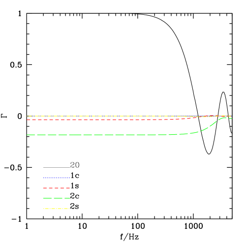
Figure 1: Overlap reduction function, as a function of the frequency, between the $m=0$ mode of a sphere at lat. $52.2^{o}$ N, long. $4.5^{o}$ E, (quantisation axis chosen along the local meridian) and the five quadrupolar modes (labelled $20$, $1c$, $1s$, $2c$, $2s$ after Zhou:1995en ) of a second sphere located at $100$ Km (lat. $52.2^{o}$ N, long. $6.0^{o}$ E, quantization axis along the local meridian).

This makes the statistics a bit different than in (21), so that for a set of $n$ spherical antennas the analogous of (20) is

$$\left[{\rm SNR}_{sphere}(2|n)\right]^{4}=\sum_{i<j\leq n}\sum_{m,m^{\prime}=1}^{5}\left[{\rm SNR}(i,m;j,m^{\prime}|2)\right]^{4}\,,$$ (31)

where the indices $i,j$ run over different detectors and $m,m^{\prime}$ run over the quadrupolar modes. If all the modes are equally noisy it is clear from fig. 1 that every mode of the first sphere can be effectively correlated with just one or two modes of the second sphere, as it has almost vanishing overlap with the others. The situation does not improve by choosing a different orientations for the quantization axis of different spheres, as an example for an angle of $45$ degrees shows in fig. 2.

At the moment the only operating spherical antenna is miniGRAIL (and another one will soon start working, the Brazilian Gravitational Wave Detector Mario Schenberg Aguiar:2005tp ), thus to obtain some numbers let us consider the present noise spectral function of miniGRAIL minigrail , whose diameter is $68$ cm. It can presently reach a strain sensitivity $h_{c}$ of about $h_{c}\equiv\sqrt{S_{h}}\sim 10^{-20}Hz^{-1/2}$, it has a resonant frequency of $2.9$kHz and a bandwidth of about $230$ Hz. For this figures one obtains, for a single pair of detectors

$$h^{2}_{100}\Omega^{95\%,5\%}_{gw}=\frac{1}{\sqrt{5}}\frac{1}{\sqrt{2T}}\frac{4\pi^{2}}{3H_{0}^{2}}\left[\int_{0}^{\infty}df\frac{\Gamma^{2}(f,x_{12})}{S_{N}^{2}(f)}\right]^{-1/2}\sim 10$$ (32)

for an observation time of 1 year. Using a set of identical spheres eq. (31) can be explicited as

$$\left[{\rm SNR}_{sphere}(2|n)\right]^{4}=2T\left(\frac{3h^{2}_{100}H_{0}^{2}}{4\pi^{2}}\right)^{2}\int_{0}^{\infty}df\frac{\Omega_{gw}^{2}(f)\sum_{i<j}\sum_{m,m^{\prime}}\Gamma^{2}(f,{x_{i,j}})}{f^{6}S_{N}^{2}(f)}\,,$$ (33)

where $S_{N}(f)$ is the common noise spectral function and $\Gamma(f,x_{i,j})$ is the overlap function for the detector pair $i-j$, which is understood to depend also on $m$ and $m^{\prime}$. The situation can be considerably improved by using larger spheres, with a consequent lower resonant frequency. We can estimate for instance that slightly improving the sensitivity to $h_{c}\simeq 10^{-21}Hz^{-1/2}$, a resonant frequency at, say, $300$ Hz (and bandwidth $100$ Hz) one can reach

$$h^{2}_{100}\Omega^{95\%,5\%}_{gw}\simeq 4\cdot 10^{-4}\times\left[5\cdot\frac{n(n-1)}{2}\right]^{-1/2}\,,$$ (34)

which is obtained by inverting (33) for a constant $\Omega_{gw}$, thus allowing to obtain $\Omega_{gw}\simeq 3\cdot 10^{-5}$ in the experiment bandwidth for a set of $n=10$ detectors. We note that it is important to have a not too high resonant frequency for detector correlation, as overlap functions go to zero at $f\gtrsim 1/\pi L$, being $L$ the detector separation. This still far from light interferometers, see eq.(29) and the phenomenological bound given by eq.(30), but the effect of the multiple correlation is quantitatively important, so it is not excluded that once higher sensitivity will be achieved the correlation effect will be crucial for detection.

The mechanism of sensitivity enhancement actually will not work if a sphere is correlated with an interferometer as only one mode of the sphere can effectively be correlated with an interferometer. This can be seen in fig. 3, which shows the overlap function between VIRGO and the five quadrupolar modes of a hypothetical sphere placed in Rome. A sphere like one with the characteristics leading to (34), has a narrower bandwidth than an interferometer, but similar sensitivity in its bandwidth, so correlating a sphere with an interferometer would lead to a result equal to (34) but for the factor in square brackets, as one cannot take advantage of the correlation of several modes of the same sphere: correlation with an interferometer would just add one more single-mode detector.

V Conclusion

We have analyzed the utility of considering multiple detector correlators to detect a stochastic background of gravitational waves. The main result of the paper is the demonstration that the best way to correlate the outputs of different detectors is in pairs, no matter how large is the number of detectors, instead of taking $m$-correlators with $m>2$. Finally as a potentially interesting application of this result we applied this strategy to a set of identical spheres, showing that correlation of several pairs of detectors is important in increasing the sensitivity.

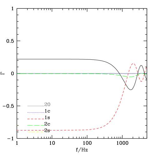
Figure 2: Overlap reduction function,as a function of the frequency, between the $m=0$ mode of a sphere at lat. $52.2^{o}$ N, long. $4.5^{o}$ E, (quantization axis along the local meridian) and the five quadrupolar modes (labelled $20$, $1c$, $1s$, $2c$, $2s$ after Zhou:1995en ) of a second sphere located at $100$ Km (lat. $52.2^{o}$ N, long. $6.0^{o}$ E, quantization axis at $45^{o}$ with respect to the local meridian).

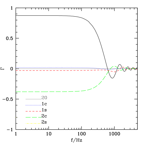
Figure 3: Overlap reduction function between VIRGO (lat. $43.6^{o}$ N, long. $10.5^{o}$ E, azimuth $160.6^{o}$ E) and the five quadrupolar modes of a hypothetical sphere located in Rome (lat. $41.8^{o}$ N, long. $12.6^{o}$ E, quantization axis at $-20^{o}$ E).

References

References

- (1) N. Christensen, Phys. Rev. D 46 (1992) 5250.
- (2) B. Allen and J. D. Romano, Phys. Rev. D 59 (1999) 102001
- (3) M. Maggiore, Phys. Rept. 331 (2000) 283
- (4) V. Ferrari, S. Matarrese and R. Schneider, Mon. Not. Roy. Astron. Soc. 303 (1999) 258
- (5) T. Damour and A. Vilenkin, Phys. Rev. D 71 (2005) 063510
- (6) C. Z. Zhou and P. F. Michelson, Phys. Rev. D 51 (1995) 2517.
- (7) A. de Waard et al.,”Progress report 2004”, Proceedings of the 5th International LISA Symposium, European Space Research and Technology Centre (ESTEC), Noordwijk, The Netherlands, Classical and Quantum Gravity (2005)
- (8) O. D. Aguiar et al., Class. Quant. Grav. 22 (2005) S209.