A Numerical Study of Boson Stars

Abstract

In this thesis we present a numerical study of general relativistic boson stars in both spherical symmetry and axisymmetry. We consider both time-independent problems, involving the solution of equilibrium equations for rotating boson stars, and time-dependent problems, focusing on black hole critical behaviour associated with boson stars.

Boson stars are localized solutions of the equations governing a massive complex scalar field coupled to the gravitational field. They can be simulated using more straightforward numerical techniques than are required for fluid stars. In particular, the evolution of smooth initial data for a scalar field tends to stay smooth, in sharp contrast to hydrodynamical evolution, which tends to develop discontinuities, even from smooth initial conditions. At the same time, relativistic boson stars share many of the same features with respect to the strong-field gravitational interaction as their fermionic counterparts. A detailed study of their dynamics can thus potentially lead to a better understanding of the dynamics of compact fermionic stars (such as neutron stars), while the relative ease with which they can be treated numerically makes them ideal for use in theoretical studies of strong gravity.

In this last vein, the study of the critical phenomena that arise at the threshold of black hole formation has been a subject of intense interest among relativists and applied mathematicians over the past decade. Type I critical phenomena, in which the black hole mass jumps discontinuously at threshold, were previously observed in the dynamics of spherically symmetric boson stars by Hawley and Choptuik [1, 2]. We extend this work and show that, contrary to previous claims, the subcritical end-state is well described by a stable boson star executing a large amplitude oscillation with a frequency in good agreement with that predicted for the fundamental normal mode of the end-state star from linear perturbation theory.

We then extend our studies of critical phenomena to the axisymmetric case, studying two distinct classes of parametrized families of initial data whose evolution generates families of spacetimes that “interpolate” between those than contain a black hole and those that do not. In both cases we find strong evidence for a Type I transition at threshold, and are able to demonstrate scaling of the lifetime for near-critical configurations of the type expected for such a transition. This is the first time that Type I critical solutions have been simulated in axisymmetry (all previous general relativistic calculations of this sort imposed spherical symmetry).

In addition, we develop an efficient algorithm for constructing equilibrium configurations of rotating boson stars, which are characterized by discrete values of an angular momentum parameter, $k$ (an azimuthal quantum number). We construct families of solutions for $k=1$ and $k=2$, and demonstrate the existence of a maximum mass in each case.

Chapter 0 Introduction

This thesis is concerned with the numerical simulation of boson stars within the framework of Einstein’s theory of general relativity. Boson stars are self-gravitating compact objects  composed of scalar particles [3], and are the bosonic counterparts of the more well-known compact fermionic stars, which include white dwarfs and especially neutron stars. In contrast to fermionic stars, there is no observational evidence that boson stars exist in nature, nor has the existence of any fundamental scalar particle yet been verified by experiments. It has been proposed, however, that boson stars could be a candidate for, or at least make up a considerable fraction of, the dark matter in our universe [4]. Were this true, it is quite probable that studies of their properties would lead to a better understanding of astrophysical phenomena. However, at the current time boson stars remain purely theoretical entities.

Their current hypothetical nature notwithstanding, boson stars might indeed exist in our universe, and, more importantly for this thesis, they are excellent matter models for the numerical study of compact objects in strong gravitational fields, a subject that continues to be a key concern of numerical relativity [5] (numerical relativity: the numerical simulation of the Einstein field equations, as well as the field equations for any matter fields being modeled). The boson stars we consider can be viewed as zero-temperature, ground-state, Bose-Einstein condensates, with enormous occupation numbers, so that the stellar material is described by a single complex scalar field, $\phi(t,{\bf x})$, that satisfies a simple, classical Klein-Gordon equation. Many of the nice modeling properties associated with boson stars derives from the fact that the dynamics is governed by a partial differential equation (PDE) that does not tend to develop discontinuities from smooth initial data. This is not the case for fermionic stars, which are usually treated as perfect fluids, and which thus satisfy hydrodynamical equations with phenomenologically-determined equations of state. Relativistic fluid evolution will generically produce shock waves and other discontinuities, even from smooth initial data. Therefore, today’s state-of-the-art relativistic hydrodynamics codes use sophisticated high resolution shock capturing (HRSC) schemes in order to more accurately and efficiently simulate the fluid physics. The fact that the solutions of the Klein-Gordon equation stay smooth is a tremendous boon when it comes to discretizing the equation in a stable and accurate manner.

In addition, the effective integration of HRSC schemes with other advanced numerical techniques such as adaptive mesh refinement [6] (AMR) is still in its infancy, at least for the case of general relativistic applications. For bosonic matter, on the other hand, it has proven relatively easy to use rather generic AMR algorithms (such as that of Berger and Oliger [6]) in conjunction with straightforward second-order finite-difference discretization to achieve essentially unbounded dynamical range in an efficient fashion [7, 8, 9].

Of course, we do not primarily study boson stars because they are easy to simulate. As mentioned already, a good fraction of the work in numerical relativity is concerned with the strong-field dynamics of gravitationally compact objects [4, 10, 11]. Despite the large amount of effort that has been devoted to this subject, it is fair to say that much remains to be learned, and much of what remains to be discovered is likely to be found through simulation. Although the strong-field gravitational physics of boson stars may not compare in detail with that of fermionic stars in all respects, there are clearly some key features of the usual stars that are shared by their bosonic counterparts. For example, in analogy with relativistic fermionic stars, spherically symmetric boson stars typically come in one-parameter families, where the parameter can be viewed as the central density of the star (or an analogue thereof). Moreover, in relativistic cases the boson star families share with the fermionic sequences the surprising property that there comes a point when increasing the density of the star at the center actually decreases the total gravitating mass of the star. In both cases this leads to maximal masses for any given family of stars. In addition, in both instances, stars near that limit are naturally very strongly self-gravitating.

Suffice it to say, then, that a careful study of general relativistic boson stars is likely to lead to insights into strong-field gravitational physics, even if there are no immediate astrophysical applications, and that this is the primary motivation for the calculations described below. In particular, and again as with the fermionic case, black hole formation is a crucial process that can, and will, generically occur in the strong-field dynamics of one or more boson stars. For the most part, this is simply because (1) as gravitationally compact objects, boson stars are, by definition, close to the point of collapse, and (2) the process of gravitational collapse involving matter with positive energy tends to be very unstable in many senses, including the fact that black hole areas can only increase.

Over the past decade or so, the careful study of gravitational collapse and black hole formation has lead to the discovery of black hole critical phenomena [7], wherein the process of black hole formation, studied in solution space, takes on many of the features of a phase transition in a statistical mechanical system. A primary goal of the work presented in this thesis is to study so-called Type I critical phenomena of boson stars in both spherical symmetry and axisymmetry, and this will be explained in more detail below. The simulations are carried out via finite difference solution of the governing PDEs. We also develop and apply a new algorithm for constructing solutions of the time-independent form of the PDEs in axisymmetry; these solutions represent relativistic rotating boson stars.

0.1 An Overview of Boson Stars

The study of boson stars can be traced back to the work of Wheeler. Wheeler studied self-gravitating objects whose constituent element is the electromagnetic field and named the resulting “photonic” configurations geons [12]. Wheeler’s original intent was to construct a self-consistent, classical and field-theoretical notion of body, thus providing a divergence-free model for the Newtonian concept of body. In the late 1960s, Kaup [3] adopted the geon idea, but coupled a massive complex scalar field, rather than the electromagnetic field, to general-relativistic gravity. Assuming time-independence and spherical symmetry he found solutions of the coupled equations which he called Klein-Gordon geons. Subsequently, Ruffini & Bonazzola [13] studied field quantization of a real scalar field and considered the ground state configurations of a system of such particles. The expectation value of the field operators gives the same energy-momentum tensor as those given by Kaup, and hence the different approaches followed in the two studies give essentially the same macroscopic results.

Later, these Klein-Gordon geons were given the name boson stars, and the nomenclature boson star now generally refers to compact self-gravitating objects that are regular everywhere and that are made up of scalar fields. Variations of the original model studied by Kaup and Ruffini & Bonazzola include self-interacting boson stars (described by a Klein-Gordon field with one or more self-interaction terms), charged boson stars (boson stars coupled to the electromagnetic field) and rotating boson stars (boson stars possessing angular momentum), to name a few. When stable, all of these objects are held together by the balance between the attractive gravitational force and a pressure that can be viewed as arising from Heisenberg’s uncertainty principle, as well as any explicit repulsive self-interaction between the bosons that is incorporated in the model. Depending on the mass of the constituent particles, and on the value of the self-interaction coupling constant(s), the size of the stars can in principle vary from the atomic scale to an astrophysically-relevant scale [10]. As mentioned previously, any given boson star is typically only one member of a continuous family of equilibrium solutions. In spherical symmetry, the family can be conveniently parametrized using the central value of the modulus of the scalar field, in analogy to the central pressure of perfect fluid stars. Moreover, the equilibrium configurations generally have an exponentially decaying tail at large distances from the stellar core, in contrast to fluid-models stars which tend to have sharp, well-defined edges.

0.1.1 Stability of Boson Stars

The dynamical stability of equilibrium, compact fermionic (fluid) stars against gravitational collapse can be studied using the linear perturbation analysis of infinitesimal radial oscillations that conserve the total particle number, $N$, and mass/energy, $M$. One important theorem in this regard concerns the transition between stable and unstable equilibrium [14][15, pp.305]. The theorem states that a perfect fluid star with constant chemical composition and constant entropy per nucleon becomes unstable with respect to some radial mode only at central densities $\rho(0)$ such that

$$\frac{\partial M(\rho(0),s,\cdots)}{\partial\rho(0)} = 0\,,$$ (1)

$$\frac{\partial N(\rho(0),s,\cdots)}{\partial\rho(0)} = 0\,.$$ (2)

In other words, a change in stability can only occur at those points in a curve of total mass $M(\rho(0))$ vs $\rho(0)$, where an extrema is attained. This results directly from the fact that the eigenvalues, $\sigma^{2}$, of the associated pulsation equation change sign at those points.

Similar results hold for various boson star models. As just mentioned, in the case of boson stars we use the central value of the scalar field modulus, denoted $\phi_{0}(0)$, as the parameter for the family of solutions, and it has been shown that the pulsation equation has a zero mode at the stationary points in the $M(\phi_{0}(0))$ plot  [16, 17]. Numerical verification of the instability of configurations past the mass maximum using the full dynamical equations in spherical symmetry was studied in [18, 19] and [2].

0.1.2 Maximum Mass of Boson Stars

As already mentioned, another important feature of stellar structure that is largely due to relativistic effects is the existence of a maximum allowable mass for a particular species of stars. Depending on the mechanism of stellar pressure (degenerate electron pressure for white dwarfs, degenerate neutron pressure for neutron stars, Heisenberg uncertainty principle for boson stars) these values are different. White dwarfs and neutron stars share the same dependence on the mass of the constituent particles ($\sim M_{\rm pl}^{3}/m^{2}$), while the dependence for boson stars is quite different ($\sim M_{\rm pl}^{2}/m$). The origin of the difference can be understood via the following heuristic argument. The ground state stationary boson stars are macroscopic quantum states of cold, degenerate bosons, whose existence is the result of the balance between the attractive gravitational force and the dispersive nature of the wave function. By the uncertainty principle, if the bosons are confined in a region of size $R$, we have $pR\sim\hbar$, where $p$ is the typical momentum of the bosons. For a moderately relativistic boson we have $p\sim mc$ and hence $R\sim\hbar/(mc)$. Equating this with the Schwarzschild radius we have $\hbar/(mc)\sim 2GM_{\mathrm{max}}/c^{2}$. Hence $M_{\mathrm{max}}\sim(\hbar c)/(2Gm)=0.5M_{\rm pl}^{2}/m$. Numerical calculation shows that $M_{\mathrm{max}}\approx 0.633M_{\rm pl}^{2}/m$ (see Sec. 0.16.4), surprisingly close to the above estimate.

The maximum mass of neutron stars can be estimated in a similar way.  The existence of these stars is the result of the balance between the attractive gravitational force and the pressure due to degenerate neutrons (fermions). Suppose there are $N$ fermions confined in a region of size $R$. Then by Pauli’s exclusion principle, each particle occupies a volume $1/n$, where $n\equiv N/R^{3}$ is the number density. Effectively, each particle has a size of $R/N^{1/3}$. Again, by the uncertainty principle we have $pR/N^{1/3}\sim\hbar$. Following the same argument as for the boson star case, we have $R\sim\hbar N^{1/3}/(mc)$, and hence $2GM_{\mathrm{max}}/c^{2}\sim\hbar N^{1/3}/(mc)\sim\hbar{M_{\mathrm{max}}}^{1/3}/(m^{4/3}c)$. Thus we have $M_{\mathrm{max}}\sim 0.35{M_{\rm pl}}^{3}/m^{2}$. In contrast to the bosonic case, then, the maximum mass of fermionic stars scales as ${M_{\mathrm{max}}}\sim{M_{\rm pl}}^{3}/m^{2}$.

0.1.3 Rotating Boson Stars

Although spherically symmetric boson star solutions were found as early as 1968, for many years it was unclear whether solutions describing time-independent boson stars with angular momentum existed or not. The first attempt to construct such stars was due to Kobayashi, Kasai & Futamase in 1994 [21]. These authors followed the same approach as Hartle and others [22, 23], in which the slow rotation of a general relativistic star is treated via perturbation of a spherically symmetric equilibrium configuration. In their study they found that slowly rotating boson stars solutions coupled with a $U(1)$ gauge field (charged boson stars) do not exist, at least perturbatively. Shortly thereafter, however, it was demonstrated that rotating boson stars could be constructed on the basis of an ansatz which leads to a quantized (or perhaps more properly, discretized) angular momentum. It was later understood that rotating boson stars have quantized angular momenta and that the concomitantly discrete nature of the on-axis regularity conditions prohibit a continuous (perturbative) change from non-rotating to rotating configurations.

A year later, Silveira & de Sousa [24], following the approach of Ferrell & Gleiser [25], succeeded in obtaining equilibrium solutions of rotating boson stars within the framework of Newtonian gravity. Specifically, they adopted the ansatz

$$\phi(t,r,\theta,\varphi)=\phi_{0}(r,\theta)e^{i\left(\omega t+k\varphi\right)}\,,$$ (3)

where $k$ is an integer (we use the symbol $k$, instead of the symbol $m$, that is commonly used in quantum mechanics, to avoid confusion with the particle mass, $m$), so that the stress-energy tensor $T^{\phi}_{\mu\nu}$ is independent of both time $t$ and the azimuthal angle $\varphi$. In the non-relativistic limit  the governing field equations constitute a coupled Poisson-Schrödinger (PS) system (for simplicity, we have dropped the subscript “0” so that $\phi_{0}(r,\theta)\to\phi(r,\theta)$)

$${\rm NewA}^{2}V=8\pi m^{2}\phi\phi^{\ast}\,,$$ (4)

$$-\frac{1}{2m}{\rm NewA}^{2}\phi+mV\phi=E\phi\,,$$ (5)

where $V$ is the Newtonian gravitational potential, and $E$ is an energy eigenvalue. The scalar field $\phi_{0}(r,\theta)$ is then expanded in associated Legendre functions, $P_{l}^{k}(\theta)$:

$$\phi_{0}(r,\theta)=\frac{1}{\sqrt{4\pi}}\sum^{\infty}_{l=k}R_{l}(r)P^{k}_{l}(\theta)\,,$$ (6)

Similarly, the potential $V(r,\theta)$ is assumed to have no $\varphi$-dependence, and thus can be expanded as

$$V(r,\theta)=\sum_{l=0}^{\infty}V_{l}(r)P_{l}(\theta)\,.$$ (7)

Eqs. (6) and (7) are then substituted into (4) and (5), and multiplied by $P_{l_{0}}(\theta)$ to obtain a system of equations for any particular value of $l_{0}$ (using the orthogonality of the associated Legendre functions). Using this strategy, Silveira and de Sousa were able to obtain solutions for each specific combination of $l_{0}$ and $k$. A main difference of these solutions relative to the spherically symmetric ones, is that the scalar field vanishes at the origin, and hence the rotating star solutions have toroidal level surfaces of the matter field, rather than spheroidal level surfaces as in the spherical case.

In 1996 Schunck & Mielke [26] used the ansatz (3) to construct rotating boson star solutions. Specifically, they chose some particular values of $k$, specifically $k=0,1\cdots,10$ and $k=500$ and showed that solutions to the fully general relativistic equations did exist for those cases. They also showed that the angular momentum, $J$, and the total particle number, $N$, of the stars are related by

$$J=kN\,,$$ (8)

where $k$ is the integer defined in (3). An important implication of the above equation is that if we consider equilibrium configurations with the same total particle number $N$, then the total angular momentum has to be quantized. This property is in clear contrast with that of a perfect fluid star.

Later, in the work most relevant to the study of rotating boson stars described in this thesis, Yoshida & Eriguchi [27] used a self-consistent-field method [28] to obtain the whole family of solutions for $k=1$, as well as part of the family for $k=2$. The maximum mass they found for the $k=1$ case was $1.314M_{\rm pl}^{2}/m$. However, their code broke down before they could compute the star with maximum mass for the $k=2$ case.

In Table 1 we summarize some similarities and differences between rotating fermion stars and rotating boson stars. For further background information on boson stars we suggest that readers consult the review by Jetzer [4], or the more up-to-date survey by Schunck & Mielke [10].

Relativistic Rotating Fermion Stars	Relativistic Rotating Boson Stars
Similarities
Come in families of solutions parametrized by a single value
Each family has a maximum possible mass
Differences
Parametrized by $p(0)$	Parametrized by $|\partial^{(k)}_{r}\phi(0)|$
Spheroidal level surfaces of rotating matter field	Toroidal level surfaces of matter field for $k=1,2,\cdots$
Finite size, abrupt change in $\partial_{r}p,\partial_{r}\rho$ at surface	Exponential decay to infinity
Angular momentum can vary continuously	Angular momentum quantized: $k=1,2,\cdots$

Table 1: Similarities and differences between relativistic rotating fermion stars and relativistic rotating boson stars.

0.2 Critical Phenomena in Gravitational Collapse

Over the past decade, intricate and unexpected phenomena related to black holes have been discovered through the detailed numerical study of various models for gravitational collapse, starting with Choptuik’s investigation of the spherically symmetric collapse of a massless scalar field [7]. These studies generally concern the threshold of black hole formation (a concept described below), and the phenomena observed near threshold are collectively called (black hole) critical phenomena, since they share many of the features associated with critical phenomena in statistical mechanical systems. The study of critical phenomena continues to be an active area of research in numerical relativity, and we refer the interested reader to the recent review article by Gundlach [29] for full details on the subject. Here we will simply summarize some key points that are most germane to the work in this thesis.

To understand black hole critical phenomena, one must understand the notion of the “threshold of black hole formation”. The basic idea is to consider families of solutions of the coupled dynamical equations for the gravitational field and the matter field that is undergoing collapse (the complex scalar field, $\phi$, in our case). Since we are considering a dynamical problem, and since we assume that the overall dynamics is uniquely determined by the initial conditions, we can view the families as being parametrized by the initial conditions—variations in one or more of the parameters that fix the initial values will then generate various solution families. We also emphasize that we are considering collapse problems. This means that we will generically be studying the dynamics of systems that have length scales comparable to their Schwarzschild radii, for at least some period of time during the dynamical evolution. We also note that we will often take advantage of the complete freedom we have as numerical experimentalists to choose initial conditions that lead to collapse, but which may be highly unlikely to occur in an astrophysical setting.

We now focus attention on single parameter families of data, so that the specification of the initial data is fixed up to the value of the family parameter, $p$. We will generally view $p$ as a non-linear control parameter that will be used to govern how strong the gravitational field becomes in the subsequent evolution of the initial data, and in particular, whether a black hole forms or not. Specifically, we will always demand that any one-parameter family of solutions has the following properties:

1. For sufficiently small values of $p$ the dynamics remains regular for all time, and no black hole forms.

2. For sufficiently large values of $p$, complete gravitational collapse sets in at some point during the dynamical development of the initial data, and a black hole forms.

From the point of view of simulation, it turns out to be a relatively easy task for many models of collapse to construct such families, and then to identify 2 specific parameter values, $p^{-}$ ($p^{+}$) which do not (do) lead to black hole formation. Once such a “bracket” $[p^{-},p^{+}]$ has been found, it is straightforward in principle to use a technique such as binary search to hone in on a critical parameter value, $p^{\star}$, such that all solutions with $p<p^{\star}$ ($p>p^{\star}$) do not (do) contain black holes. A solution corresponding to $p=p^{\star}$ thus sits at the threshold of black hole formation, and is known as a critical solution. It should be emphasized that underlying the existence of critical solutions are the facts that (1) the end states (infinite-time behaviour) corresponding to properties 1. and 2. above are distinct (a spacetime containing a black hole vs a spacetime not containing a black hole) and (2) the process characterizing the black hole threshold (i.e. gravitational collapse) is unstable. We also note that we will term evolutions with $p<p^{\star}$ subcritical, while those with $p>p^{\star}$ will be called supercritical.

Having discussed the basic concepts underlying black hole critical phenomena, we now briefly describe the features of critical collapse that are most relevant to the work in this thesis.

First, critical solutions do exist for all matter models that have been studied to date, and for any given matter model, almost certainly constitute discrete sets. In fact, for some models, there may be only one critical solution, and we therefore have a form of universality.

Second, critical solutions tend to have additional symmetry beyond that which has been adopted in the specification of the model (e.g. we will impose spherical and axial symmetry in our calculations).

Third, the critical solutions known thus far, and the black hole thresholds associated with them, come in two broad classes. The first, dubbed Type I, is characterized by static or periodic critical solutions (i.e. the additional symmetry is a continuous or discrete time-translational symmetry), and by the fact that the black hole mass just above threshold is finite (i.e. so that there is a minimum black hole mass that can be formed from the collapse). The second class, called Type II, is characterized by continuously or discretely self-similar critical solutions (i.e. the additional symmetry is a continuous or discrete scaling symmetry), and by the fact that the black hole mass just above threshold is infinitesimal (i.e. so that there is no minimum for the black hole mass that can be formed). The nomenclature Type I and Type II is by analogy with first and second order phase transitions in statistical mechanics, and where the black hole mass is viewed as an order parameter.

Fourth, solutions close to criticality exhibit various scaling laws. For example, in the case of Type I collapse, where the critical solution is an unstable, time-independent (or periodic) compact object, the amount of time, $\tau$, that the dynamically evolved configuration is well approximated by the critical solution per se satisfies a scaling law of the form

$$\tau(p)\sim-\gamma\ln|p-p^{\star}|\,,$$ (9)

where $\gamma$ is a universal exponent in the sense of not depending on which particular family of initial data is used to generate the critical solution, and $\sim$ indicates that the relation (9) is expected to hold in the limit $p\to p^{\star}$.

Fifth, and finally, much insight into critical phenomena comes from the observation that although unstable, critical solutions tend to be minimally unstable, in the sense that they tend to have only a few, and perhaps only one, unstable modes in perturbation theory. In fact, if one assumes that a Type I solution, for example, has only a single unstable mode, then the growth factor (Lyapunov exponent) associated with that mode can be immediately related to the scaling exponent $\gamma$ defined by (9).

In this thesis we will be exclusively concerned with Type I critical phenomena, where the threshold solutions will generally turn out to be unstable boson stars. Previous work relevant to ours includes studies by (1) Hawley [1] and Hawley & Choptuik [2] of boson stars in spherically symmetry, (2) Noble [30] of fluid stars in spherical symmetry and (3) Rousseau [31] of axisymmetric boson stars within the context of the conformally flat approximation to general relativity. Evidence for Type I transitions have been found in all three cases.

0.3 Layout

The remaining chapters of this thesis are organized as follows. In Chap. A Numerical Study of Boson Stars we summarize the mathematical formalism used in the work of this thesis. This includes a brief summary of the mathematical model of spacetime, in which the key ingredient to be used is the Einstein field equation. We then summarize the ADM (3+1) formalism, which will be used in the study of boson stars in spherical symmetry, as well as the (2+1)+1 formalism, which is used in the study of boson stars in axisymmetry. We also describe the Einstein-Klein-Gordon system, which is the fundamental set of PDEs underlying all of our studies.

In Chap. A Numerical Study of Boson Stars we summarize the numerical methods used in the thesis. This includes finite differencing techniques which are central to all the calculations shown; the multigrid method, which is used in the construction of rotating boson stars, as well as in the solution of the constraint equations in the dynamical study of boson stars in axisymmetry; adaptive mesh refinement, which is essential in the study of critical phenomena in axisymmetry; excision techniques which are used in the study of boson stars in spherical symmetry; and the technique of spatial compactification, which is used in the construction of rotating boson stars.

In Chap. A Numerical Study of Boson Stars we study Type I critical phenomena of boson stars in spherical symmetry. This research can be viewed as an extension of the work reported by Hawley & Choptuik in [2]. Our principal new result is compelling numerical evidence for the existence of oscillatory final states of subcritical evolutions. We also perform perturbation analyses and show that the simulation results agree very well with those obtained from perturbation theory. We then present a rudimentary, but stable and convergent implementation of the black hole excision method for the model. Supercritical simulations using excision show that the spacetimes approach static black holes at late time, so there is no impediment to very long run times (in physical time).

In Chap. A Numerical Study of Boson Stars we describe a study of boson stars in axisymmetry. We first present an algorithm to construct the equilibrium configurations of rotating boson stars that is based on the multigrid technique. We argue that our method is more computationally efficient than methods previously used and reported in the literature. More importantly, we obtain numerical solutions in the highly relativistic regime for an angular momentum parameter $k=2$. We then discuss studies of the dynamics of boson stars in axisymmetry. Following Choi’s [32] work in the Newtonian limit, we show that solitonic behaviour occurs in the head-on collision of boson stars with sufficiently large relative initial velocities. We also present a study of Type I critical phenomena in the model. The two classes of simulations (collisions of boson stars, and boson stars gravitationally perturbed by a massless real scalar field) provide evidence for Type I black hole transitions, as well as scaling laws for the lifetime of near-critical configurations of the form (9). This represents the first time that Type I behaviour has been observed in the context of axisymmetric collapse.

The final chapter summarizes the results, gives overall conclusions and points to some directions of future work. Several appendices providing various technical details are also included.

0.4 Conventions, Notation and Units

Throughout this thesis the signature of metric is taken to be ($-$ + + +). Spacetime indices of four dimensional (1 temporal + 3 spatial) tensors are labeled by lower case Greek letters ($\alpha,\beta,\gamma,\cdots$). Spatial indices of three dimensional (3 spatial) tensors are labeled by lower case Latin letters starting from $i$ ($i,j,k,\cdots$). Spacetime indices of three dimensional (1 temporal + 2 spatial) tensors are labeled by the first few Latin indices ($a,b,c,\cdots,h$), and spatial indices of two dimensional (2 spatial) tensors are labelled by upper case Latin letter ($A,B,C,\cdots$). The Einstein summation convention is implied for all types of indices. That is, repeated (one upper and one lower) indices are automatically summed over the appropriate range. Covariant derivatives are denoted by ${\rm NewA}$ or by a semi-colon “;”. Ordinary partial derivatives are denoted by $\partial$ or by a comma “,”. Conventions for the Riemann and Ricci tensors are ${\rm NewA}_{[\alpha}{\rm NewA}_{\beta]}V_{\gamma}=\frac{1}{2}R_{\alpha\beta\gamma\delta}V^{\delta},R_{\mu\nu}=R^{\alpha}{}_{\mu\alpha\nu}$.

We adopt a system of “natural” units in which $G=c=\hbar=1$. In this system the unit time, unit length and unit mass are known as the Planck time, Planck length and Planck mass, respectively. Specifically, we have

$$T_{\rm{pl}} = \sqrt{\frac{\hbar G}{c^{5}}}=5.39\times 10^{-44}\mbox{s}\,,$$ (10)

$$L_{\rm{pl}} = \sqrt{\frac{\hbar G}{c^{3}}}=1.62\times 10^{-35}\mbox{m}\,,$$ (11)

$$M_{\rm{pl}} = \sqrt{\frac{\hbar c}{G}}=2.18\times 10^{-8}\mbox{kg}\,.$$ (12)

The corresponding energy scale is $M_{\rm{pl}}\,c^{2}\approx 10^{19}\mbox{GeV}$. For the scalar field, the action has dimension $[\hbar]$. Hence $\left[d^{4}x(\partial\phi)^{2}\right]=[\hbar]$. Therefore, $[\phi]=[\sqrt{\hbar}]/L=\sqrt{M/T}$. Thus, $\phi$ is measured in units of $\sqrt{M_{\rm{pl}}/T_{\rm{pl}}}=6.36\times 10^{17}\sqrt{\mbox{kg/s}}$.

Finally, we adopt a nomenclature commonly used in numerical work, whereby we refer to calculations requiring the solution of partial differential equations in $n$ spatial dimensions as “$n$D”. In particular, we will often refer to spherically symmetric computations (whether time-dependent or not) as “1D”, and axisymmetric calculations (again, irrespective of any time-dependence) as “2D”.

Chapter 0 Mathematical Formalism

In this chapter we briefly summarize the mathematical description of spacetime, as well as the ADM (or 3+1) and (2+1)+1 decompositions of spacetime. These decompositions—which form the bases for the numerical calculations described in the remainder of this thesis—are well described in the literature, and we therefore restrict our discussion here to a summary of the physical picture, and statements of the key equations that will be used in subsequent chapters.

0.5 Mathematical Model of Spacetime

In general relativity the elementary entities are events, each of which is characterized by a time, $t$, and location, $x^{i}$, at which the particular event occurs. According to Einstein’s geometric view of the gravitational interaction, gravitational physics is concerned with the relationship between these events: in other words, it describes the “structure” of a collection of events $\mathcal{M}=\{(t,x^{i})\}$. Specifically, we are to view the collection of events as a surface with a certain structure imposed on it. In mathematical language, the collection of events forms a manifold, where manifold is simply a generalization of the concept of surface, and the structure that describes the gravitational physics turns out to be a metric on the manifold. The pair of objects, the manifold, $\mathcal{M}$, and the metric, $g_{\mu\nu}$, comprise spacetime, which is of primary interest in general relativity. The study of spacetime thus becomes the study of the explicit form of the metric, or, equivalently, of the geometry of spacetime.

The physics that we are looking for should also tell us how the distribution of matter affects the structure of spacetime. In other words, the theory should have a way of prescribing matter fields, and the relationship between these matter fields and the geometry of spacetime. Mathematically, we describe the matter as some tensor fields on the manifold, and the relationship between the matter and the geometry is written in the form of field equations. We will make some further assumptions about the spacetime so that some general physical principles—of whose validity we are confident—will be satisfied. Following Hawking and Ellis [33], these assumptions are:

1. Local causality: special relativity posits that no signal can travel faster than the speed of light. Therefore, equations for any matter fields should respect this property. Causality effectively partitions the neighborhood of any point $p$ into two sets: those points which are causally connected to $p$ and those which are not. This assumption allow us to determine the metric up to a conformal factor (i.e. up to an overall location-dependent scale).

2. Local conservation of energy and momentum: conservation laws generally reflect symmetries in physical laws. Energy and momentum conservation—related to invariance of physical laws under temporal and spatial translations—is a cornerstone of physics, with an extremely solid empirical basis. Conservation of energy and momentum can be expressed as a condition on the energy-momentum tensor, $T_{\mu\nu}$, which describes the matter content of the spacetime. Knowledge of this tensor determines the conformal factor. In general the conservation equations would not be satisfied for a connection derived from a metric $\hat{g}=\Omega^{2}g$. Observing two paths $\gamma(t)$ and $\gamma^{\prime}(t)$ of small test particles would allow us to determine $\Omega$ up to a constant factor, which simply reflects one’s units of measurement.

3. Field equations: this is the most stringent assumption that we make, but it also yields the key equation that we wish to solve, namely the Einstein field equation:

   $$G_{\mu\nu}\equiv R_{\mu\nu}-\frac{1}{2}g_{\mu\nu}R=8\pi T_{\mu\nu}\,.$$ (1)

   Here $G_{\mu\nu}$, $R_{\mu\nu}$ and $R$ are, respectively, the Einstein tensor, the Ricci tensor and the Ricci scalar. (We note that, in contrast to [33], we further assume that the cosmological constant vanishes.) We observe that predictions made on the basis of this equation agree, within experimental/observational uncertainties, with all experiments and observations that have been performed to date. (A survey of experimental tests of general relativity can be found in [34], and an up-to-date review of the state of the art in experimental verification of the theory is given in [35, 36]). The Einstein equation is the mathematical expression of the statement that “matter tells spacetime how to curve”. In turn, the curvature of spacetime “tells matter how to move” through the appearance of the metric, and gradients of the metric in the equations of motion for the matter fields.

0.6 The ADM (3+1) Formalism

One of the great conceptual revolutions of relativity is the unification of the concepts of space and time into a single entity. This unification is partly motivated by the fact that, under general coordinate transformations, time and space “mix” together, and it is thus no longer meaningful to talk about absolute space or absolute time. In particular, the field equation (1), which is invariant under general coordinate transformations, relates the entire spacetime geometry to the distribution of matter-energy in space and time. The value of physics, on the other hand, is often rooted in its ability to predict what happens in the future, given certain information that is known at some initial time (where time must generally be defined with respect to a given family of observers). In other words, one traditional way of solving a physics problem is through the study of the dynamics of the system under consideration; i.e. given the state of a physical system at a specific instant of time, we use dynamical equations of motion to evolve the state to yield information about the system at future (or past) times. This approach of viewing the solution of (1) as the time development of some initial data is known as the Cauchy problem for relativity. Note that realization of this strategy will in some sense undo Einstein’s feat of unification, i.e. it will split up spacetime into 3 “space” dimensions plus 1 “time” dimension—hence the terminology “3+1” split. The split will involve the introduction of some specific coordinate system, including a definition of time, and a prescription of initial data at the specified initial time. The initial data are to be chosen so that, as much as possible, the resulting evolution will accurately model the physical system of interest. We will then march the data forward in time using the dynamical form of the field equation. Our task then, is to rewrite equation (1) as a set of partial differential equations (PDEs) suitable for solution as a dynamical problem. As it turns out, the PDEs themselves naturally decompose into two classes: one which involves only quantities defined at a given instant of time (the constraints), and another that describe how the dynamical variables evolve in time (evolution equations).

The split of spacetime into space and time as sketched above, was first introduced by Arnowitt, Deser and Misner [37, 38] (hence the name ADM formalism). The original motivation for the development of the formalism was, in fact, the desire to cast the field equations in a form suitable for quantization. Although this so-called canonical quantization of the gravitational field remains a largely unsolved problem, the ADM approach has proven to be a very useful basis for classical computations in numerical relativity.

The explicit 3+1 decomposition proceeds as follows. We suppose that spacetime is orientable, which, roughly speaking means that we can time order the events in spacetime. We then slice up the spacetime into different slices of constant time, and label each slice with a value of the time parameter, $t$. We demand that the slicing is such that any two events on any given slice are spacelike-separated; i.e. that the slices are spacelike hypersurfaces . The collection of these slices $\{\Sigma_{t}\}$ becomes a particular “foliation” of spacetime. Mathematically this foliation is described, at least locally, by a closed one form, $\Omega=dt$ (the closed nature of the form enables us to use $t$ as a unique label for the slice). The norm (length) of this form quantifies how far (proper distance) it is from one slice, $\Sigma_{t}$, to a nearby slice, $\Sigma_{t+dt}$:

$$\|\Omega\|^{2}\equiv g^{\mu\nu}\Omega_{\mu}\Omega_{\nu}\equiv-\alpha^{-2}\,\,.$$ (2)

Here, the positive function, $\alpha$, is called the lapse function and encapsulates one of the four degrees of coordinate freedom in the theory. The unit-normalized one form, $n_{\mu}$

$$n_{\mu}=-\alpha\Omega_{\mu}\,,$$ (3)

and the associated unit-norm vector, $n^{\mu}=g^{\mu\nu}n_{\nu}$, then allow us to define a projection operator, $\perp^{\mu}{}_{\nu}$

$$\perp^{\mu}{}_{\nu}\equiv\delta^{\mu}{}_{\nu}+n^{\mu}n_{\nu}\,.$$ (4)

Note that since $n^{\mu}$ is timelike, we have $g_{\mu\nu}n^{\mu}n^{\nu}=g^{\mu\nu}n_{\mu}n_{\nu}=n^{\mu}n_{\mu}=-1$. Using the projection operator, we can construct tensors that “live in” the hypersurfaces by projecting all of the indices of generic 4-dimensional (spacetime) tensors. For example, for a rank-3 tensor with one contravariant and two covariant indices, we can define

$$\perp T^{\alpha}{}_{\beta\gamma}\equiv\perp^{\alpha}{}_{\kappa}\perp^{\mu}{}_{\beta}\perp^{\nu}{}_{\gamma}T^{\kappa}{}_{\mu\nu}\,.$$ (5)

By construction, any tensor defined in this fashion is orthogonal to the unit normal, so that, for example, we have $n_{\alpha}\perp T^{\alpha}{}_{\beta\gamma}=n^{\beta}\perp T^{\alpha}{}_{\beta\gamma}=n^{\gamma}\perp T^{\alpha}{}_{\beta\gamma}=0$. Hence such a tensor naturally lives in the 3-dimensional hypersurfaces, and is known as a spatial tensor. In particular, we construct the induced (or spatial) metric, $\gamma_{\mu\nu}$, via

$$\gamma_{\mu\nu}\equiv\perp g_{\mu\nu}=g_{\mu\nu}+n_{\mu}n_{\nu}\,,$$ (6)

and note that $\gamma_{\mu\nu}$ describes the intrinsic geometry of the hypersurfaces. Similarly, we can use projection to define a 3-covariant derivative, $D_{\alpha}$, that is compatible with the 3-metric, $\gamma_{\mu\nu}$ (i.e. so that $D_{\alpha}\gamma_{\mu\nu}=0$). For example, for a spatial vector, $V^{\mu}$ ($V^{\mu}n_{\mu}=0$), we have

$$D_{\alpha}V^{\mu}\equiv\perp\nabla_{\alpha}V^{\mu}=\perp^{\beta}{}_{\alpha}\perp^{\mu}{}_{\nu}\nabla_{\beta}V^{\nu}\,,$$ (7)

where $\nabla_{\alpha}$ is the spacetime covariant derivative. Using $D_{\alpha}$ and standard formulae of tensor calculus, we can then compute the various 3-dimensional curvature tensors (Riemann tensor, Ricci tensor, Ricci scalar etc.) that characterize the geometry of the hypersurfaces.

In the 3+1 approach, the components of the 3-metric, $\gamma_{\mu\nu}$, are to be viewed as dynamical variables of the theory; the geometry of spacetime then becomes the time history of the geometry of an initial hypersurface. In order to characterize how the geometries of two nearby slices differ, we must consider the manner in which the slices are embedded in the enveloping spacetime. This information is encoded in the (symmetric) extrinsic curvature tensor, which, up to a sign, is simply the projected gradient of the unit normal to the hypersurfaces:

$$K_{\mu\nu}=K_{\nu\mu}\equiv-\perp{\rm NewA}_{\mu}n_{\nu}\,.$$ (8)

From the above definition, it is clear that $K_{\mu\nu}$ is a spatial tensor, and thus can also be viewed as living in the hypersurfaces. Roughly speaking, the components of the extrinsic curvature can be thought of as the velocities (time derivatives) of the 3-metric components (see equation (17)), so that $\gamma_{\mu\nu}$ and $K_{\mu\nu}$ are, loosely, dynamical conjugates. With the above definitions of the spatial metric and the extrinsic curvature (also known as the first and second fundamental forms, respectively), one can derive the Gauss-Codazzi equations 

$$\perp R_{\alpha\beta\gamma\delta} = {}^{(3)}R_{\alpha\beta\gamma\delta}+K_{\delta\beta}K_{\gamma\alpha}-K_{\gamma\beta}K_{\delta\alpha}\,,$$ (9)

$$\perp R_{\alpha\beta\gamma\hat{n}} = D_{\beta}K_{\alpha\gamma}-D_{\alpha}K_{\beta\gamma}\,,$$ (10)

where ${}^{(3)}R_{\alpha\beta\gamma\delta}$ denotes the Riemann tensor constructed from the spatial metric, $\gamma_{\mu\nu}$, and where, following York [38], a $\hat{n}$ in a covariant index position denotes that the index has been contracted with $n^{\mu}$—for instance, $W_{\hat{n}}\equiv W_{\mu}n^{\mu}$. (However, and again following York, a $\hat{n}$ in a contravariant index position denotes contraction with $-n_{\mu}$.)

The Einstein equation, together with the following definitions:

$$\rho \equiv T_{\hat{n}\hat{n}}=T_{\mu\nu}n^{\mu}n^{\nu}\,,$$ (11)

$$j^{\mu} \equiv \perp T^{\mu\hat{n}}=-\perp\left(T^{\mu\nu}n_{\nu}\right)\,,$$ (12)

where $T^{\mu\nu}$ is again the stress energy tensor, allow us to rewrite the Gauss-Codazzi equations as

$${}^{(3)}R+K^{2}-K_{ij}\,K^{ij}=16\pi\rho\,\,,$$ (13)

$$D_{j}K^{ij}-D^{i}K=8\pi j^{i}\,\,.$$ (14)

Here, ${}^{(3)}R$ is the 3-dimensional Ricci scalar, $K\equiv\gamma^{ij}K_{ij}$ is the trace of $K_{ij}$ and we remind the reader that Latin indices range over the spatial values $1,2,3$. We also note that spatial indices on spatial tensors are raised and lowered using $\gamma^{ij}$ and $\gamma_{ij}$, respectively, and that $\gamma_{ij}\gamma^{jk}=\delta^{i}{}_{k}$.

(13) and (14) involve only spatial tensors and spatial derivatives of such tensors, and hence, from the point of view of dynamics, represent constraints that must be satisfied on each slice, including the initial slice. They are commonly called the Hamiltonian constraint and momentum constraint respectively, and are a direct consequence of the four-fold coordinate freedom of the theory.

So far we have used only one coordinate degree of freedom, which was in our specification of the manner in which we foliated the spacetime into a family of spacelike hypersurfaces—or, equivalently, in the specification of the lapse function, $\alpha$, at all events of the spacetime. For any fixed time slicing, however, we are allowed to relabel the spatial coordinates of events intrinsic to any of the slices as illustrated in Fig. 1. As shown in that figure, it is convenient to describe the general labeling of events with spatial coordinates relative to the specific labelling one would get by propagating the spatial coordinates along the unit normal field, $n^{\mu}$. In general, the spatial coordinates, will be “shifted” relative to normal propagation, and this shift will be quantified by a spatial vector, $\beta^{\mu}$, known, naturally enough, as the shift vector. An observer who is at rest with respect to the coordinate system illustrated in Fig. 1 will thus move along a worldline with a tangent vector given by

$$t^{\mu}=\alpha n^{\mu}+\beta^{\mu}\,,$$ (15)

where we again emphasize that $\beta^{\mu}n_{\mu}=0$.

The specification of the three independent components of the shift vector, along with the lapse function exhausts the coordinate freedom of general relativity, and defines a coordinate system $(t,x^{i})$ (sometimes called a 3+1 coordinate system) that we will assume covers the region of spacetime in which we are interested. In such a coordinate system, and using a four-dimensional generalization of the Pythagorean theorem, we can then write the spacetime displacement in 3+1 form

$$ds^{2}=(-\alpha^{2}+\beta_{i}\beta^{i})\,dt^{2}+2\beta_{i}\,dt\,dx^{i}+\gamma_{ij}\,dx^{i}\,dx^{j}\,\,.$$ (16)

Figure 1: This figure illustrates a schematic representation of the ADM, or 3+1, decomposition. $\alpha$ is the lapse function and encodes the proper distance, $\alpha dt$, between two infinitesimally separated hypersurfaces, $\Sigma(t)$ and $\Sigma(t+dt)$. $\beta^{i}$ is the shift vector and describes the shifting of spatial coordinates, $x^{i}$, relative to normal propagation. $PP^{\prime\prime}$ is the vector $t^{\mu}=\alpha n^{\mu}+\beta^{\mu}$, where $n^{\mu}$ is the unit timelike normal to the hypersurfaces, and is proportional to the 4-velocity of an observer with fixed spatial coordinates.

From the definitions of the vector field, $t^{\mu}$ (15), and the extrinsic curvature (8), one can show that

$$\pounds_{t}\gamma_{ij}=-2\alpha K_{ij}+D_{i}\beta_{j}+D_{j}\beta_{i}\,\,,$$ (17)

where $\pounds_{t}$ denotes Lie differentiation along $t^{\mu}$ (in a 3+1 coordinate system $\pounds_{t}$ reduces to partial differentiation $\partial_{t}$). This last expression can be viewed as a set of evolution equations for the 3-metric components, and makes the interpretation of the extrinsic curvature components as “velocities” of the $\gamma_{ij}$ manifest.

Making the further definitions

$$S_{\mu\nu} \equiv \bot T_{\mu\nu}\,,$$ (18)

$$S \equiv \gamma^{ij}S_{ij}\,,$$ (19)

the remaining components of the Einstein equation can be written as:

$$\pounds_{t}\,K_{ij} = -D_{i}D_{j}\,\alpha+\alpha\left\{{}^{(3)}R_{ij}-2K_{ik}K^{k}{}_{j}+K_{ij}K-8\pi\left[S_{ij}-\frac{1}{2}\gamma_{ij}\,\left(S-\rho\right)\right]\right\}$$ (20)

$$+\beta^{k}{D}_{k}K_{ij}+K_{ik}{D}_{j}\beta^{k}+K_{kj}{D}_{i}\beta^{k}\,,$$

where ${}^{(3)}R_{ij}$ is the 3-dimensional Ricci tensor. These last equations are to be viewed as evolution equations for the extrinsic curvature components.

In summary, the 3+1 decomposition applied to the Einstein field equation (1) yields a set of 4 constraint equations, (13), (14), and 12 (first order in time) evolution equations, (17) and (20). We note that, as a consequence of the contracted Bianchi identity (which itself follows from the coordinate invariance of the theory), the evolution equations guarantee that data that satisfies the constraints at some instant in time (at the initial time, for example), is evolved to data that satisfies the constraints at any future or past times.

We conclude this section by observing that a key idea in the 3+1 approach is to use a timelike vector field, $n^{\mu}$ (whose existence is guaranteed by the Lorentzian signature of the spacetime metric), to construct a projection operator that is then used to define quantities on surfaces orthogonal to $n^{\mu}$ (surfaces of simultaneity), and to derive equations governing those quantities from the covariant field equations. This same idea is used in the (2+1)+1 formalism described in the next section, the only difference being that we will now decompose with respect to a spacelike vector field, $\xi^{\mu}$, which is a Killing vector field.

0.7 The (2+1)+1 Formalism

Suppose we stack a collection of identical planar figures—such as the text string “(2+1)+1”—to create a 3-dimensional structure as shown in Fig. 2. For the purposes of discussion, we will think of the 3-dimensional object as being of infinite extent in the $z$-direction. To describe this structure it suffices to state that its $z={\rm const.}$ cross section is the planar text “(2+1)+1”, and that it has a symmetry in the $z$ direction. Similarly if there is a symmetry in spacetime, we can state what the symmetry is, then focus on the detailed structure of a “cross section” orthogonal to the symmetry direction. This technique of “dividing out” the symmetry and then restricting attention to the cross section, or projected space, (or, in mathematical parlance, the quotient space ), underlies the (2+1)+1 formalism. In particular, if the spacetime in which we are interested is axisymmetric, we can first project quantities and equations onto a “plane” perpendicular to this symmetry, and then perform the equivalent of an ADM space-plus-time decomposition on the dimensionally reduced spacetime.

Figure 2: A 3-dimensional object with continuous symmetry, which can be described as having a cross section that is the planar text string “(2+1)+1”, and which has a symmetry along the $z$ direction.

The (2+1)+1 formalism described here is based on the work of Maeda and his collaborators [39], and, as just stated, combines (1) the method of dimensional reduction (dividing out the symmetry, or projection along the symmetry) of a spacetime possessing a Killing vector field, as originally developed by Geroch [40], and (2) a 3-dimensional analogue of the ADM approach introduced in the previous section (Sec. 0.6). Other references for the application of this formalism to problems in numerical relativity include [41, 8].

As previously mentioned, we are interested in the case of axisymmetry, and thus assume that the spacetime under consideration contains a spacelike Killing vector field, $\xi^{\mu}$, with closed orbits. Choosing an azimuthal coordinate, $\varphi$, adapted to the symmetry, the Killing vector can be written as:

$$\xi^{\mu}\equiv\left(\frac{\partial}{\partial\varphi}\right)^{\mu}\,.$$ (21)

To perform the projection, we first construct a projection operator, ${\mathcal{H}}^{\alpha}{}_{\beta}$, similar to that previously used in the 3+1 decomposition :

$$\mathcal{H}^{\alpha}{}_{\beta}\equiv\delta^{\alpha}{}_{\beta}-\frac{\xi^{\alpha}\xi_{\beta}}{\xi^{\gamma}\xi_{\gamma}}\,.$$ (22)

Using this operator, we can construct tensors intrinsic to the cross sections via projections of spacetime tensors. In particular, we can project the spacetime metric itself (or equivalently, lower the contravariant index of ${\mathcal{H}}^{\alpha}{}_{\beta}$) to yield the metric, ${\mathcal{H}}_{\alpha\beta}$, on the dimensionally reduced space:

$$\mathcal{H}_{\alpha\beta}\equiv g_{\alpha\beta}-\frac{\xi_{\alpha}\xi_{\beta}}{\xi^{\gamma}\xi_{\gamma}}\,.$$ (23)

Again paralleling the 3+1 development, we can also use projection of the spacetime covariant derivative, $\nabla_{\alpha}$, to define an induced covariant derivative operator, $D_{\alpha}$, in the cross sections that satisfies $D_{\alpha}{\mathcal{H}}_{\mu\nu}=0$.

Since it is a (Lorentzian) metric on a 3-dimensional manifold, ${\mathcal{H}}_{\alpha\beta}$ clearly has fewer degrees of freedom than the spacetime metric, $g_{\alpha\beta}$. The “missing” degrees of freedom can be conveniently encoded in the norm, $s$, and the twist, $\omega^{\alpha}$, of the Killing vector, $\xi^{\mu}$:

$$s^{2} \equiv \xi^{\alpha}\xi_{\alpha}\,,$$ (24)

$$\omega^{\alpha} \equiv \epsilon^{\alpha}{}_{\beta\gamma\delta}\,\xi^{\beta}\xi^{\delta;\gamma}\,.$$ (25)

where $\epsilon^{\alpha}{}_{\beta\gamma\delta}$ is the usual Levi-Civita symbol. Note that since $\omega_{\alpha}\xi^{\alpha}=\mathcal{L}_{\xi}\omega_{\alpha}=\mathcal{L}_{\xi}s^{2}=0$, $s^{2}$ and $\omega_{\alpha}$ are tensors intrinsic to the cross sections. For notational convenience, we further define

$$\omega^{2} \equiv \omega^{\alpha}\omega_{\alpha}\,,$$ (26)

$$\lambda \equiv s^{2}\,.$$ (27)

The basic equations for a spacetime with a Killing vector field $\xi^{\alpha}$ can now be written as :

$$D_{[\alpha}\omega_{\beta]} = -\epsilon_{\alpha\beta\gamma\delta}\,\xi^{\gamma}R^{\delta}{}_{\epsilon}\,\xi^{\epsilon}\,,$$ (28)

$$D^{\alpha}\omega_{\alpha} = \frac{3}{2\lambda}\omega_{\beta}D^{\beta}\lambda\,,$$ (29)

$$D^{2}\lambda = \frac{1}{2\lambda}D^{\alpha}{\lambda}D_{\alpha}{\lambda}-\frac{\omega^{2}}{\lambda}-2R_{\alpha\beta}\xi^{\alpha}\xi^{\beta}\,,$$ (30)

$${\mathcal{R}}_{\alpha\beta} = \frac{1}{2\lambda^{2}}\left(\omega_{\alpha}\omega_{\beta}-{\mathcal{H}}_{\alpha\beta}\omega^{2}\right)+\frac{1}{s}D_{\alpha}D_{\beta}s+{\mathcal{H}}^{\mu}{}_{\alpha}{\mathcal{H}}^{\nu}{}_{\beta}R_{\mu\nu}\,,$$ (31)

where ${\mathcal{R}}_{\alpha\beta}$ denotes the Ricci tensor associated with the induced metric ${\mathcal{H}}_{\alpha\beta}$. Note that (28)–(31) completely describe the dimensional reduction piece of the (2+1)+1 formalism, and are written in purely geometrical terms. To incorporate matter fields, we can manipulate (28)–(31) and use the Einstein equation to get:

$$D_{[a}\omega_{b]} = 8\pi s\,\epsilon_{abc}\tau^{c},$$ (32)

$$D^{a}\left[\frac{\omega_{a}}{s^{3}}\right] = 0\,,$$ (33)

$$\frac{1}{s}D^{2}s = -\frac{\omega^{2}}{2s^{4}}-4\pi\left(\frac{T_{\phi\phi}}{s^{2}}-\tau\right),$$ (34)

$${\mathcal{G}}_{ab}\equiv{\mathcal{R}}_{ab}-\frac{1}{2}{\mathcal{H}}_{ab}{\mathcal{R}} = 8\pi{\cal T}_{ab}\,,$$ (35)

where ${\mathcal{R}}={\mathcal{H}}^{ab}{\mathcal{R}}_{ab}$. Here we note that indices $a,b,\cdots$ range over the temporal and (two) spatial dimensions of the reduced space, and that we have defined the following quantities:

$$\tau_{ab} \equiv {\mathcal{H}}^{\gamma}{}_{a}{\mathcal{H}}^{\delta}{}_{b}\,T_{\gamma\delta}\,,$$ (36)

$$\tau^{c} \equiv {\mathcal{H}}_{\alpha}{}^{c}\,T^{\alpha}{}_{\phi}\,,$$ (37)

$$\tau \equiv T-\frac{T_{\phi\phi}}{s^{2}}\,,$$ (38)

$${\mathcal{T}}_{ab} \equiv \tau_{ab}-\frac{1}{4}{\mathcal{H}}_{ab}\left(\tau-\frac{T_{\phi\phi}}{s^{2}}\right)+\frac{1}{8\pi}\left\{\frac{\omega_{a}\omega_{b}}{2s^{4}}+\frac{1}{s}\left[D_{a}D_{b}s-\frac{1}{2}{\mathcal{H}}_{ab}D^{2}s\right]\right\}.$$ (39)

Note that the 4-dimensional Einstein equations have been effectively replaced by (32)–(35), where the first two equations determine the twist $\omega^{a}$ , the third equation determines the norm, $s$, of the Killing vector field, and the fourth governs the reduced metric, ${\mathcal{H}}_{\alpha\beta}$.

The last stage in the derivation of the (2+1)+1 equations involves a space-plus-time split (completely analogous to the 3+1 split) of the reduced field equations. Again, the interested reader is referred to [39] for full details.

0.8 Boson Stars—the Einstein-Klein-Gordon System

In this section we briefly describe the theoretical framework for boson stars, which are equilibrium configurations of a massive, complex Klein-Gordon field coupled to gravity—we will thus refer to the model as the Einstein-Klein-Gordon system.

We derive the equations for the Einstein-Klein-Gordon system using a variational approach. The model is described by an action

$$S=\int d^{4}x\sqrt{-g}\,\left(\mathcal{L}_{g}+\mathcal{L}_{\phi}\right)\,,$$ (40)

where

$$\mathcal{L}_{g}\equiv\frac{1}{16\pi}R\,,$$ (41)

and

$$\mathcal{L}_{\phi}\equiv-\frac{1}{2}\left({\rm NewA}^{\mu}\phi{\rm NewA}_{\mu}\phi^{\ast}+m^{2}|\phi|^{2}\right)\,.$$ (42)

Here $R$ is the spacetime Ricci scalar and $\phi$ is a massive complex scalar field with bare (particle) mass $m$. Variation of the action with respect to the metric $g_{\mu\nu}$ yields the Einstein equation

$$R_{\mu\nu}-\frac{1}{2}g_{\mu\nu}R=8\pi T_{\mu\nu}\,,$$ (43)

where

$$T_{\mu\nu}\equiv T^{\phi}_{\mu\nu}\equiv\frac{1}{2}\left[\left({\rm NewA}_{\mu}\phi{\rm NewA}_{\nu}\phi^{\ast}+{\rm NewA}_{\nu}\phi{\rm NewA}_{\mu}\phi^{\ast}\right)-g_{\mu\nu}\left(\ {\rm NewA}^{\alpha}\phi{\rm NewA}_{\alpha}\phi^{\ast}+m^{2}|\phi|^{2}\right)\right]\,.$$ (44)

Similarly, variation with respect to the field $\phi$ gives the Klein-Gordon equation

$${\rm NewA}^{\mu}{\rm NewA}_{\mu}\phi-m^{2}\phi=0\,.$$ (45)

The coupled equations (43) and (45) constitute the equations of motion for the Einstein-Klein-Gordon system, and, in particular, are the fundamental equations used in our subsequent study of boson stars. When we (gravitationally) perturb boson stars using an additional real, massless scalar field, $\phi_{3}$, we simply add an extra term $\mathcal{L}_{\phi_{3}}$ to the total Lagrangian density

$$\mathcal{L}=\mathcal{L}_{g}+\mathcal{L}_{\phi}+\mathcal{L}_{\phi_{3}}\,,$$ (46)

with

$$\mathcal{L}_{\phi_{3}}\equiv-\frac{1}{2}{\rm NewA}^{\mu}{\rm NewA}_{\mu}\phi_{3}\,.$$ (47)

This yields an additional contribution, $T_{\mu\nu}^{\phi_{3}}$, to the total stress energy tensor

$$T_{\mu\nu}=T_{\mu\nu}^{\phi}+T_{\mu\nu}^{\phi_{3}}\,,$$ (48)

where

$$T_{\mu\nu}^{\phi_{3}}={\rm NewA}_{\mu}\phi_{3}{\rm NewA}_{\nu}\phi_{3}-\frac{1}{2}g_{\mu\nu}\ {\rm NewA}^{\alpha}\phi_{3}{\rm NewA}_{\alpha}\phi_{3}\,,$$ (49)

as well as a field equation (the massless Klein-Gordon equation), for $\phi_{3}$

$${\rm NewA}^{\mu}{\rm NewA}_{\mu}\phi_{3}=0\,.$$ (50)

In the following chapters we will consider more explicit forms of the above equations of motion, once we have imposed symmetries and fixed specific coordinate systems.

Chapter 0 Numerical Methods

In this chapter we briefly summarize the numerical methods used in this thesis, as well as some continuum strategies central to our numerical calculations. As with the previous chapter, since most of the topics discussed here are well documented in the literature, we refer the interested reader to appropriate references for additional details. We also note that we use the common subscript notation for partial differentiation, e.g. $u_{x}\equiv\partial u/\partial x$, in this chapter.

0.9 Finite Difference Techniques

The basic technique that we use in our computational solution of model physical problems is finite differencing. Finite differencing is a very commonly used method in the numerical solution of partial differential equations (PDEs), and continues to dominate work in numerical relativity. The basic idea of the approach is to replace partial derivatives by suitable algebraic difference quotients, and the fundamental assumption underlying the efficacy of the technique is that the functions to be approximated are smooth so that they can be Taylor-expanded about any point in the computational domain. The first step in the development of a finite difference approximation (FDA) to a PDE (or more generally, to a system of PDEs) is the introduction of a discrete grid (or lattice, or mesh) of points, which replaces the continuum physical domain. We then approximate continuum field quantities ${\bf u}=\left(u,v,w,\cdots\right)$ by a set of grid functions ${{\bf u^{h}}}=(u^{h},v^{h},w^{h},\cdots)$ which will constitute a solution of our FDA. For simplicity of presentation, we will now assume that our vector of fields, ${\bf u}$, has a single component, $u(t,x)$, which is a function of time and one spatial dimension, but the approach and techniques discussed in the following are easily generalized to the cases of multiple fields and/or multiple spatial dimensions.

We will generally restrict attention to so-called uniform grids wherein the spacing between adjacent grid points is constant in each of the coordinate directions. Denoting these regular mesh spacings in space and time as $h$ and $k$, respectively, and assuming that we are solving our PDE on the continuum domain, $x_{\rm min}\leq x\leq x_{\rm max}$, $t\geq 0$, our finite difference grid is given by $(x_{j},t^{n})$, where

$$x_{j}=x_{\rm min}+\left(j-1\right)h\,,\,\,j=1,\cdots,N_{x}\,,$$ (1)

with

$$h=\frac{x_{\rm max}-x_{\rm min}}{N_{x}-1},$$ (2)

and

$$t^{n}=nk\,,\,\,n=0,1,\cdots\,.$$ (3)

For any grid function $u^{h}\in{\bf u^{h}}$, the value at $(x_{j},t^{n})$ is denoted by $u^{n}_{j}$ and is an approximation of the continuum value $u(x_{j},t^{n})$. Convergence of the finite difference approximation is then the statement that $\lim_{h\to 0,k\to 0}u^{n}_{j}=u(x_{j},t^{n})$. We remark at this point that, operationally, investigation of the behaviour of a finite difference solution, $u^{h}$, as a function of the mesh spacings $h,k$ (holding other problem parameters fixed) provides a very powerful and general methodology for assessing the accuracy of the solution. We have used this strategy of convergence testing extensively in assessing the correctness and accuracy of the results described in later chapters. In addition, for all of our time-dependent calculations, when we vary the spatial mesh spacing(s) during a convergence test, we also vary the time step, $k$, so that (for the one dimensional case), the ratio $\lambda=k/h$ is held constant ($\lambda$ is often called the Courant factor, or Courant number). Thus, our FDAs tend to be characterized by a single overall discretization scale.

We now sketch one general technique that can be used to derive finite difference formulae. As mentioned above, we want to use difference quotients (algebraic combinations of grid-function values) to approximate derivatives. For instance, suppose we wish to approximate the first derivative $u_{x}(x)$ of our function $u(x)$. Suppressing the time index, $n$, we Taylor series expand about $x=x_{j}$

$$u_{j+ih}=[u]_{j}+ih[u_{x}]_{j}+\frac{1}{2}(ih)^{2}[u_{xx}]_{j}+O(h^{3})\,,$$ (4)

for $i=-I,\cdots,-2,-1,0,1,2,\cdots,\tilde{I}$. Now suppose we want to use a three-point formula (or a three-point stencil) to calculate our approximation of the first derivative (see Fig. 1).

Figure 1: A 3-point finite difference stencil suitable for computation of a second-order approximation to a first derivative

We consider a linear combination, $\sum_{i=-1}^{1}c_{i}u_{j+ih}$, of the grid function values at the grid points $x_{i-1},x_{i},x_{i+1}$, and equate it to the first derivative, $u_{x}$, evaluated at $x=x_{j}$:

$$\sum_{i=-1}^{1}c_{i}u_{j+ih}\sim[u_{x}]_{j}\,.$$ (5)

Solving for the coefficients $c_{i}$, we find

$$c_{-1} = -\frac{1}{2h}\,,$$

$$c_{0} = 0\,,$$ (6)

$$c_{1} = +\frac{1}{2h}\,,$$

and hence our FDA is

$$u_{x}(x_{j})=\frac{u_{j+1}-u_{j-1}}{2h}+O(h^{2})\,.$$ (7)

Since the truncation error of this formula is $O(h^{2})$, we call the approximation second order. Similarly, we can derive expressions for other derivatives (with varying degrees of accuracy) using appropriate stencils. For example, we have [42]

$$u_{x}(x_{j}) = \frac{u_{j+1}-u_{j}}{h}+O(h)\,,$$ (8)

$$u_{x}(x_{j}) = \frac{u_{j}-u_{j-1}}{h}+O(h)\,,$$ (9)

$$u_{xx}(x_{j}) = \frac{u_{j+1}-2u_{j}+u_{j-1}}{h^{2}}+O(h^{2})\,,$$ (10)

$$u_{xx}(x_{j}) = \frac{-u_{j+2}+16u_{j+1}-30u_{j}+16u_{j-1}-u_{j-2}}{12h^{2}}+O(h^{4})\,.$$ (11)

In discretizing time-dependent PDEs we make exclusive use of Crank-Nicholson schemes, with second order spatial differences. For the case of one space dimension (1+1 problems), such a scheme uses the stencil shown in Fig. 2:

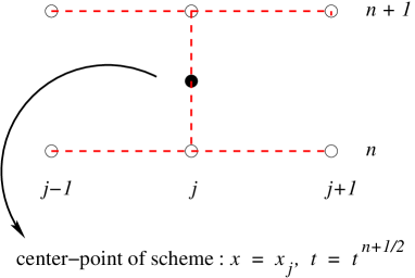
Figure 2: Stencil for an $O(h^{2})$ Crank-Nicholson scheme for a PDE in one space dimension and time.

The key idea of a Crank-Nicholson method is to keep the differencing centered in time as well as in space. As an example, we consider the simple advection equation

$$u_{t}(t,x)=au_{x}\,,$$ (12)

where $a$ is a constant. The Crank-Nicholson scheme for the equation is then

$$\frac{u^{{}^{\scriptstyle n+1}}_{{}_{\scriptstyle j}}-u^{{}^{\scriptstyle n}}_{{}_{\scriptstyle j}}}{\Delta t}=\frac{a}{2}\,\left[\frac{u^{{}^{\scriptstyle n}}_{{}_{\scriptstyle j+1}}-u^{{}^{\scriptstyle n}}_{{}_{\scriptstyle j-1}}}{2\Delta x}+\frac{u^{{}^{\scriptstyle n+1}}_{{}_{\scriptstyle j+1}}-u^{{}^{\scriptstyle n+1}}_{{}_{\scriptstyle j-1}}}{2\Delta x}\right]\,,$$ (13)

and is $O(\Delta t^{2},\Delta x^{2})$ accurate as can be verified via Taylor series expansion about the center-point of the stencil, $(x_{j},t^{n+1/2})$ (see Fig. 2). Note that the scheme involves the FDA of the spatial derivative applied at both the retarded ($n$) and advanced ($n+1$) time levels. This leads to coupling of the advanced-time unknowns, $u^{n+1}_{j}$ (i.e. the scheme is implicit), and is crucial for both the accuracy and stability of the scheme.

The Crank-Nicholson approach can be applied in a straightforward manner to any set of time-dependent PDEs that have been cast in first-order-in-time form, and for the case of the evolution equations treated in this thesis, the discrete equations that result can be solved iteratively in an efficient manner.

For time-dependent FDAs, the notions of convergence and stability are intimately related. We have generally not encountered serious stability problems with the difference schemes used below, but nonetheless refer the interested reader to [43] for discussion of this important subject.

0.10 Multigrid Method

In this section we introduce the basic concepts and techniques of the multigrid method for the solution of FDAs arising from the discretization of elliptic boundary value problems. This method (including a modification for eigenvalue problems) is used extensively in our construction of stationary solutions describing rotating boson stars, and in the solution of the elliptic constraint equations and coordinate conditions that arise in our study of the dynamical evolution of axisymmetric boson stars. A more detailed introductory discussion of the method can be found in [44, 45], while [46] provides an extensive reference source.

Traditional methods for solving elliptic PDEs, such as successive over-relaxation (SOR), are easy to implement, but suffer from slow convergence rates (particularly in the limit of small mesh sizes), and have contributed to the general impression that, relative to equations of evolutionary type, the finite difference solution of elliptic equations is computationally expensive. However, the multigrid method, first introduced by Brandt in the 1970s [47], is capable of solving discrete versions of elliptic PDEs (even systems of nonlinear PDEs) in a time that is proportional to the total number, $N$, of grid points in the discretization—i.e. in $O(N)$ time. The basic idea underlying multigrid is to use a hierarchy of grids with different resolutions (mesh spacings) to solve a particular problem instead of using a single grid. By an intelligent transfer of the problem back and forth between the various grids, one can speed up the convergence rate of the solution process on the finest grid. Central to the efficient operation of most multigrid solvers is the observation that straightforward relaxation (in particular, Gauss-Seidel relaxation, [45, 48]) is very good at removing high frequency error components, but very bad at removing low frequency ones. At the same time, once the solution error has been smoothed by relaxation, we can sensibly pose a coarse grid version of the problem at hand, the solution of which can be computed in a fraction of the time required to solve the fine grid problem.

Perhaps the best way of illustrating the multigrid method is by consideration of a simple example. Suppose we want to solve the following linear elliptic equation

$$Lu=f\,,$$ (14)

where $L$ is some linear elliptic operator, $u$ is the continuum solution, and $f$ is a source function (we assume $L$ is linear strictly to keep the presentation simple; as already mentioned, the multigrid technique can also be applied to nonlinear elliptic equations). As in the previous section we replace the PDE by a finite difference approximation, defined on a uniform grid characterized by a mesh spacing, $h$

$$L^{h}u^{h}=f^{h}\,.$$ (15)

Here $L^{h}$ is our FDA of $L$ and $u^{h}$ and $f^{h}$ are the grid versions of the solution and source function, respectively. Suppose we have an approximate solution (or guess) $\tilde{u}^{h}$ to the above equation. Then we consider the difference, $v^{h}$, between the exact discrete solution, $u^{h}$, and the (current) approximation, $\tilde{u}^{h}$, to $u^{h}$:

$$v^{h}=u^{h}-\tilde{u}^{h}\,.$$ (16)

We call $v^{h}$ the error or correction, since it is the quantity by which we must correct $\tilde{u}^{h}$, so that we get the solution of the finite difference approximation. Solving this last expression for $u^{h}$, and substituting the result in (15) we have

$$L^{h}\left(\tilde{u}^{h}+v^{h}\right)=f^{h}\,,$$ (17)

or

$$L^{h}v^{h}=-\left(L^{h}\tilde{u}^{h}-f^{h}\right)\equiv-r^{h}\,,$$ (18)

where we have defined the residual or defect, $r^{h}$. Focus is now shifted to the solution of (18) for the correction, $v^{h}$. Once $v^{h}$—or more generally, some approximate solution, ${\tilde{v}}^{h}$, of (18)—is in hand, we can update $\tilde{u}^{h}$ via

$$\tilde{u}^{h}:=\tilde{u}^{h}+v^{h}\,.$$ (19)

Of course, (18) is fundamentally no easier to solve than (15). However, if we apply a few relaxation sweeps to (18), thus smoothing the residual, $r^{h}$, as well as the (unknown) correction, $v^{h}$, we can transfer the problem to a coarser grid with mesh size $H$, where $H$ is a multiple of $h$ (typically $H=2h$). That is, we consider the coarse grid problem

$$L^{H}v^{H}=-r^{H}=-I_{h}^{H}r^{h}\,,$$ (20)

where the coarse grid source function, $r^{H}$, is obtained by the application of a suitable restriction operator $I_{h}^{H}$ to the fine grid residual, $r^{h}$ (i.e. $I_{h}^{H}$ transfers a fine grid function to a coarse grid).

Particularly for 2D and 3D cases, the coarse grid problem will be significantly less expensive to solve than the fine grid problem. Once the solution $v^{H}$ is obtained we can approximate the desired correction $v^{h}$ by using an prolongation operator, $I^{h}_{H}$, which transfers a coarse grid function to a fine grid:

$$\tilde{v}^{h}\equiv I^{h}_{H}v^{H}\,,$$ (21)

Once the fine grid function has been updated using the prolonged correction, a few more relaxation sweeps are applied to smooth out any high frequency error components that are introduced in the coarse-to-fine transfer of the correction.

We note that the choice of suitable restriction and prolongation operators will generally depend on the discretization that is used, as well as on the specific type of relaxation strategy that is employed to smooth the residuals/corrections. More importantly, the above sketched process of a two level correction can be easily generalized to a multi-level correction, wherein one uses an entire hierarchy of mesh scales (for example $h,2h,4h,\cdots$) and where the cost of solving the discrete equations on the coarsest grid can be made computationally negligible. The algorithmic process by which the solution is manipulated first on the finest grid, then on the auxiliary coarse grids, and finally on the finest grid again is called a multigrid cycle. Although it is sometimes advantageous to use other types of cycles, we use $V$-cycles exclusively in our work, wherein the problem solution sequence is $l_{f},l_{f}-1,\cdots,l_{c}+1,l_{c},l_{c}+1,\cdots l_{f}-1,l_{f}$, and where the integers $l_{c}$ and $l_{f}$ ($l_{f}>l_{c}$) label the coarsest and finest levels, respectively, of refinement used.

0.11 Adaptive Mesh Refinement

In this section we introduce the method of adaptive mesh refinement (AMR). This method is important in the finite difference solution of problems that exhibit significant variation in the length and time scales that must be resolved (dynamic range), particularly when the specific resolution requirements (e.g. in which regions of the computational domain the smallest scale features will develop) are not known a priori.

In numerical relativity, the use of AMR has played a crucial role in the study of black hole critical phenomena, one class of which is characterized by self-similar solutions, which thus involve features on arbitrarily small scales (see [7] for example). Other examples where AMR is likely to ultimately play an important role include the calculations aimed at predicting the gravitational waves generated from the inspiral and merger of a black hole binary. Here one basic length scale is set by the mass, $M$, of one of the holes (we assume roughly equal mass black holes)—clearly, in the vicinity of the black holes our finite difference mesh must be sufficiently fine to resolve that length scale. On the other hand, the gravitational waves that are generated in the late stages of the binary evolution will have wavelengths of order $10M$, and the computational grid may have to extend to a distance of order $100M$ from the sources in order that the wave train that would register in a terrestrial detector can be accurately read off. Use of a single uniform grid with $h$ chosen small enough to resolve the smallest scale features would not only be extremely inefficient in such a case, it would likely be prohibitively expensive (both in terms of CPU time and memory), even with the largest computers currently available.

One can attempt to deal with the multi-scale nature of such a problem through the use of a non-uniform grid (or several component grids, each of which is uniform) so that the local mesh spacing at least roughly matches the local resolution requirement. Here we are envisioning the use of a priori information concerning the nature of the solution, and would further assume that the resolution demands are static, so that, for example, the regions requiring highest resolution would not move around during the course of the solution. Such a refinement strategy is often known as fixed mesh refinement (FMR) and has been used successfully in some recent calculations in numerical relativity (see, for instance, [49, 50]). However, in many situations—such as the modeling of objects that propagate through the computational domain—we will not have detailed a priori information concerning the resolution requirements, and thus algorithms that adaptively respond to the local development of solution features become attractive. Note that such algorithms need to have the capability both to introduce additional resolution when and where it is needed and to coarsen the local discretization scale when and where resolution demands become less stringent.

Here we briefly describe the version of AMR introduced by Berger and Oliger in 1984 [6], which has been previously extended to accommodate the treatment of elliptic equations and then incorporated into the axisymmetric code, graxi [8, 9, 51, 52], used to generate the results discussed in Chap. A Numerical Study of Boson Stars. We note that the graxi implementation of AMR introduces several simplifying restrictions relative to the original Berger and Oliger work—the most important of these include the requirements that (1) the computational domain be covered by a single base-level grid, (2) all component grids be aligned with the coordinate axes, (3) each level, $l$, of refinement be characterized by a unique spatial discretization scale, $h_{l}$, (4) the refinement factor between any two successive discretization levels be a unique integer $\rho$, and (5) distinct grids at the same level are not allowed to overlap.

The Berger and Oliger algorithm was designed for the finite difference solution of general systems of hyperbolic partial differential equations. Adaptivity is achieved via the use of a hierarchy of component grids, where each component has uniform mesh spacings in each of the coordinate directions (and in our case, the same mesh spacing in all directions). Specifically, the hierarchy is characterized by a sequence of discretization levels, $l=0,1,2,\cdots l_{\rm max}$, where $l=0$ represents the coarsest level of grid, and $l_{\rm max}$ the finest. Associated with each level is a spatial discretization scale, $h_{l}$, and the scales at different levels satisfy

$$h_{l}\equiv\rho h_{l+1}\,,$$ (22)

where $\rho\geq 2$ is an integer (typically 2 in our calculations). The grid hierarchy can be denoted $G_{l,j}$, where the index $l$ ranges over the discretization levels, while the index $j$, for each level, ranges over the number of component grids at that level. At the coarsest level, $l=0$, there is only a single grid, $G_{0,0}$, which covers the entire computational domain. At finer levels, $l\geq 1$, there can be an arbitrary number of grids each of which is required to (1) have extrema ($x_{\rm min},x_{\rm max},y_{\rm min}$ etc.) that coincide with mesh points of some level $l-1$ grid, and (2) be completely contained within that grid. The level $l-1$ grid, $G_{l-1,j^{\prime}}$ that contains $G_{l,j}$ is called the parent grid, while $G_{l,j}$ is known as a child of $G_{l-1,j^{\prime}}$. As mentioned previously, distinct grids at the same level are not allowed to overlap.

Fig. 3 shows a schematic representation of a typical grid hierarchy for a 1+1 dimensional problem with $l_{\rm max}=2$ and a refinement ratio $\rho=2$. Note that the mesh refinement occurs in time as well as in space, and that the discrete time steps, $k_{l}$, used in the various levels of the hierarchy satisfy

$$k_{l}\equiv\rho k_{l+1}\,,$$ (23)

(i.e. a constant Courant factor is maintained across the hierarchy). Also notice that the structure of the hierarchy changes in time—resolution is increased where needed through the introduction of new grids, and decreased where it is not needed through the deletion of one or more existing grids.

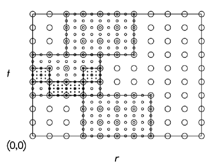
Figure 3: Schematic representation of a typical grid structure for a 1+1 calculation using Berger and Oliger adaptive mesh refinement (AMR). In this figure we have $l_{\mathrm{max}}=2$ and $\rho=2$.

The core of the Berger and Oliger algorithm is a recursive time stepping algorithm whereby equations on coarse grids are advanced before those on fine grids. This allows the fine grid values at so-called refinement boundaries (i.e. boundaries of grids $G_{l,j},l>0$ that do not coincide with boundaries of the global computational domain) to be computed via interpolation of parental values. Otherwise the same set of finite difference equations (including discretized versions of the physical boundary conditions) are used to update discrete unknowns on all component grids. Once a single time step has been completed at level $l$, and if any level $l+1$ grids exist, the recursive time stepping algorithm is invoked to take $\rho$ steps at level $l+1$, so that the fine grid equations are integrated to the same physical time as the coarse ones.

Another key component of the AMR algorithm is the regridding procedure in which resolution demands are periodically assessed, and the grid hierarchy is correspondingly reconfigured. The crucial task here is to decide when and where a particular solution region requires refinement or coarsening. Although other approaches are possible, graxi implements the strategy described in [6] that ties regridding to local (truncation) error estimates based on Richardson-type procedures. To illustrate this method, assume that our FDA can be written as

$$u^{n+1}=Q^{h}u^{n}\,,$$ (24)

where $u^{n+1}$ and $u^{n}$ are the advanced ($t=t^{n+1}$) and retarded ($t=t^{n}$) finite difference unknowns, respectively (spatial grid indices are suppressed), and $Q^{h}$ is the finite difference update operator that advances the solution from one discrete time to the next. We can then generate a local estimate of the solution error by taking two time steps on the base mesh, characterized by discretization scale $h$, and then comparing the result to what we get by advancing the retarded data by one step on a coarsened mesh with discretization scale $2h$. That is we compute

$$e^{h}\equiv\left(Q^{h}Q^{h}-Q^{2h}\right)u^{n}\,,$$ (25)

where the coarse grid update operator $Q^{2h}$ employs the same FDA as $Q^{h}$. (This technique is directly analogous to the procedure commonly used in adaptive ordinary differential equation (ODE) integrators.) This error estimation can be performed dynamically and makes use of the same FDA that is used in the basic time stepping procedure previously described. We also note that the technique can be applied independently of the particular PDE being solved or the specific difference technique that is being used.

Once the error estimate is calculated, we can determine those grid points where the error estimate exceeds some predefined tolerance. These points are then organized into clusters and the regridding procedure is carried out. This includes creation of a new grid hierarchy (or some portion of it), transfer of values from the old hierarchy to the new, and interpolation of grid function values from parental to child grids for those spatial locations where a given level of refinement did not previously exist.

A final key aspect of the Berger and Oliger algorithm involves the fine-to-coarse transfer of values from level $l$ child grids to their level $l-1$ parents once the level $l$ integration has been advanced to the time of the level $l-1$ solution. Were this not done, the level $l-1$ values coinciding with refined regions—which by definition are not of sufficient accuracy to satisfy the error control criterion—would eventually “pollute” level $l-1$ values in regions that should, in principle, not require refinement.

Again, the reader who is interested in further details of this AMR algorithm can consult [6, 8].

0.12 Excision Techniques

Starting in the 1960s, R. Penrose and S. Hawking proved a series of theorems which are now collectively called the singularity theorems. The essential implication of these theorems is that physical singularities are generic features of spacetime, and are not a consequence, for example, of symmetries that a specific spacetime might possess. In particular, these mathematically rigorous results, as well as the results from detailed numerical simulation of gravitational collapse make it clear that black holes invariably contain physical singularities. This fact has proven to be of enormous significance for the numerical simulation of black hole spacetimes. At singularities physical quantities become undefined and it is meaningless to evolve spacetime there.  It thus seems to be an unavoidable conclusion that numerical simulations must somehow avoid black hole singularities. The traditional approach in numerical relativity (used in virtually all calculations prior to the early 1990’s) was to use coordinate freedom to accomplish singularity avoidance. For instance the maximal slicing condition (described in more detail in Chap. A Numerical Study of Boson Stars), whereby the trace of the extrinsic curvature tensor is required to vanish at all times, generates slices that automatically “slow down time” in the vicinity of a black hole singularity, essentially freezing the evolution before the singularity is encountered. Unfortunately, singularity-avoiding coordinate systems generically become pathological (i.e. coordinate pathologies develop) on dynamical time scales, and this typically leads to a breakdown of simulations (i.e. the code “crashes” due to an inability to resolve extremely steep gradients etc.). Thus the use of singularity avoiding coordinates alone does not appear to provide an effective resolution to the problem of long-time evolution of black hole spacetimes.

An alternate approach to singularity avoidance that has become quite popular over the past decade or so is based on an idea due to Unruh (see [53] for a discussion of the method). Unruh argued in the early 1980’s that since the interiors of black holes are causally disconnected from the exterior universe, it is not necessary (and is in fact wasteful) to evolve regions inside black holes when our main interest is in the exterior region of spacetime. He thus proposed that one excise the interiors of black holes from the computational domain. However, since the location of a black hole surface—the event horizon—requires knowledge of the complete spacetime, one cannot in principle excise a black hole until the global solution is in hand. Unruh’s second suggestion was thus to use the location of an apparent horizon (which one can very loosely view as an instantaneous approximation to the intersection of an event horizon with a given spacelike hypersurface) as the excision surface. Black hole excision was first explored numerically by Thornburg [53], while the first successful implementation of the method in a dynamical context was due to Seidel and Suen [54]. Some other recent references that discuss excision include [55, 56, 57, 58, 59, 60, 61, 62, 63]. We will describe this method in more detail in section 0.18.

0.13 Spatial Compactification

In this section we discuss issues related to compactification of a spatial domain. This technique is used in the construction of the stationary boson star solutions described in Sec. 0.16.3 and Sec. 0.20. For simplicity of presentation we assume here that the domain to be compactified is 1-dimensional.

The principal motivating factor for using a compactified spatial domain is the desire to use exact, rather than approximate, boundary conditions in the solution of our PDEs. Specifically, for the problems considered in Sec. 0.16.3 and Sec. 0.20, we know the exact boundary conditions at spatial infinity, $r=\infty$, whereas we generally know only the asymptotic behaviour of given functions at any specific finite distance, $r_{\rm max}$. Moreover, even if we know the exact form (e.g. precise falloff conditions) for our functions, it may be computationally advantageous to work with Dirichlet conditions (as the conditions at infinity tend to be), rather than the mixed (Robin) boundary conditions that typically result from the use of known falloff behaviour. We thus would like to explore one class of transformations that allows us to perform compactification.

Suppose we want to compactify $r\in[0,\infty)$ to $\zeta\in[a,b]$ via the following transformation:

$$\zeta(r)=\frac{f(r)}{1+f(r)}\,,$$ (26)

where $f(r)$ is some arbitrary function of $r$. To ensure $\zeta(0)=a$ and $\zeta(\infty)=b$, we have

$$f(0) = \frac{a}{1-a}\,,$$ (27)

$$f(\infty) = \frac{b}{1-b}\,.$$ (28)

We also wish the coordinate transformation to be regular, so that

$$\frac{d\zeta}{dr}=\frac{f^{\prime}}{(1+f)^{2}}\neq 0\,,$$ (29)

or simply

$$f^{\prime}\neq 0\,.$$ (30)

In other words, $f$ should be a strictly increasing (or decreasing) function of $r$. (27), (28) and (30) are the only restrictions on a general compactifying function $f$. However, as we will see in Sec. 0.20 when we consider the generation of initial data representing rotating boson stars, once we have fixed coordinates, we find that as the angular momentum of the star increases, the location of the extremum of the solution moves towards a boundary of the computational domain. In addition, for larger angular momentum values, the solution function becomes increasingly peaked, which means that for fixed solution accuracy and coordinates, finer resolution is required as the angular momentum increases. Thus, in addition to compactifying the domain, we attempt to map the location of the function extremum to the central region of the computational domain.

We therefore impose the additional conditions that the coordinate transformation map some arbitrary points, $r_{i}$, to some given values $\zeta_{i}$. We then have

$$f(r_{i})=\frac{\zeta_{i}}{1-\zeta_{i}}\,,$$ (31)

where $i=0,\cdots,N$. If we assume $b=1$, then one such possibility is to write

$$f(r) = \alpha_{0}+\alpha_{1}r+\alpha_{2}r^{2}+\cdots$$ (32)

$$= \sum_{i}\alpha_{i}r^{i}\,,$$

whereby $\alpha_{i}$ can be chosen to satisfy conditions (27) and (31). More specifically, if we want to compactify the radial coordinate to $[0,1]$, and we want to bring one particular point $r=r_{0}$ (say the location where the grid function is a maximum) to $\zeta=1/2$, then $\alpha_{0}=0$, $\alpha_{1}=1/r_{0}$ and $\alpha_{2}=\alpha_{3}=\cdots=0$; i.e. we have

$$\zeta(r) = \frac{\alpha_{1}r}{1+\alpha_{1}r}$$ (33)

$$= \frac{r}{r_{0}+r}\,.$$

In other words, transformation (33) maps $[0,\infty)$ to $[0,1]$ with $\zeta(r_{0})=\frac{1}{2}$.

Chapter 0 Boson Stars in Spherical Symmetry

In this chapter we study boson stars in spherical symmetry. In spherically symmetric spacetime the equations of motions are greatly simplified, and with a proper choice of coordinates the number of variables that must be evolved is significantly reduced. Therefore it is relatively easy to study the system numerically compared to higher dimensional (2-dimensional and 3-dimensional) simulations. At the same time, of all of the symmetries that could be imposed to reduce the field equations to a set of PDEs in one space dimension and time, spherical symmetry is clearly the most appropriate for the study of isolated, gravitationally compact objects.

This chapter consists of two parts. The first part concerns the construction of static solutions which represent spherically symmetric boson stars in the ground state. These solutions provide the initial data for the simulations of critical phenomena of boson stars in spherical symmetry studied in the second part of this chapter, as well as for the simulation of critical phenomena of boson stars in axisymmetry in Chap. A Numerical Study of Boson Stars. Together with rotating solutions computed in the Newtonian limit, the solutions also provide initial guesses in the construction of the general relativistic, stationary, rotating boson star solutions which will also be described in Chap. A Numerical Study of Boson Stars.

The second part of the chapter concerns the dynamics of spherical boson stars. More specifically, in an extension of the work performed by Hawley and Choptuik [2], we study the critical phenomena of boson stars which are driven to the threshold of black hole formation via an external perturbing agent. As in the previous work, our boson stars are perturbed by a real massless scalar field and an overall amplitude of this real scalar field is used to tune to criticality. However, we use a different coordinate system—maximal-isotropic coordinates—than that used in [2]. Although the accuracy of finite difference calculations in any given coordinate system can in principle be estimated using intrinsic means (e.g. convergence tests), we feel that it is nonetheless useful to reproduce the calculations of [1, 2] in a different coordinate system. In addition, since maximal-isotropic coordinates can penetrate black hole horizons (the polar-areal coordinates used in [2] generally cannot), we can also implement black hole excision in our simulations. We emphasize however, that we feel that our excision calculations—which are restricted to spherical symmetry and use an ad hoc boundary condition at the excision surface for the lapse—are only a minor result of the thesis.

The principal new results presented in this chapter concern the long-time evolutions of subcritical simulations in critical collapse of boson stars. We provide numerical evidence that—contrary to the previous conjecture [2] that subcritical solutions disperse most of the original mass of the boson star to large distances—the late time behaviour of subcritical evolution is characterized by oscillation about a stable boson star solution. We also apply a linear perturbation analysis similar to that in [2] and confirm that the observed oscillation modes agree with the fundamental modes given by perturbation theory. (We use a code provided by S. Hawley [64] to generate the frequencies from the perturbation analysis.) We also observe that there is generically an overall lower-frequency modulation of the post-critical-phase oscillations. At this time we have no explanation for the origin of this additional oscillatory behaviour, although we can safely rule out the possibility that it originates from the beating between the fundamental and first harmonic mode.

The outline of the remainder of the chapter is as follows. In Sec. 0.14 we derive the equations of motion for boson stars in a general spherically symmetric spacetime. In Sec. 0.15 we specialize the equations of motion to maximal-isotropic coordinates. In Sec. 0.16 we derive systems of equations for the initial value problem in maximal-isotropic coordinates, polar-areal coordinates and compactified maximal-isotropic coordinates, and briefly describe the family of stationary solutions that we can generate using any of the three approaches. In Sec. 0.17 we present the results of near-critical evolutions and, for the case of subcritical evolutions, compare the oscillatory behaviour observed at late times to that predicted from perturbation theory. Finally in Sec. 0.18 we study the implementation of black hole excision technique applied to our system. Throughout this chapter we denote ${}^{\prime}\equiv\partial_{r}$ and $\dot{}\equiv\partial_{t}$, and $m=1$ is used for the particle mass of the boson field.

0.14 Spherically Symmetric Spacetime

Loosely speaking, we may regard a spherically symmetric spacetime as one that admits a preferred timelike observer such that the spacetime is spherically symmetric about every point on this special observer’s world-line.  The most general metric for a time-dependent spherically-symmetric spacetime can be written as [65, 66, 67]

$$ds^{2}=\left(-\alpha^{2}+a^{2}\beta^{2}\right)dt^{2}+2a^{2}\beta\,dtdr+a^{2}dr^{2}+r^{2}b^{2}d\Omega^{2}\,,$$ (1)

where $d\Omega^{2}\equiv d\theta^{2}+\sin^{2}\theta\,d\varphi^{2}$ is the metric on the unit 2-sphere, $\beta$ is the $r$-component of the shift vector, $\beta^{i}=\left(\beta,0,0\right)$, and $\alpha,\beta,a,b$ are functions of $t$ and $r$ only. Corresponding to the above metric is an extrinsic curvature tensor with only two independent components 

$$K^{i}{}_{j}={\mbox{diag}}\left(K^{r}\,_{r},K^{\theta}\,_{\theta},K^{\theta}\,_{\theta}\right)\,,$$ (2)

where $K^{r}{}_{r}$, $K^{\theta}{}_{\theta}$ are also functions of $t$ and $r$. Together with $\alpha,\beta,a$ and $b$ we thus must deal with a maximum of 6 out of 16 possible geometrical variables in spherically symmetric calculations. The 4-metric can be written in matrix form as

$$g_{\mu\nu}=\left[\begin{array}[]{cccc}-\alpha^{2}+a^{2}\beta^{2}&a^{2}\beta&0&0\\ a^{2}\beta&a^{2}&0&0\\ 0&0&(rb)^{2}&0\\ 0&0&0&(rb\sin\theta)^{2}\end{array}\right]\,,$$ (3)

from which it immediately follows that the inverse metric is given by

$$g^{\mu\nu}=\left[\begin{array}[]{cccc}-1/\alpha^{2}&\beta/\alpha^{2}&0&0\\ \beta/\alpha^{2}&1/a^{2}-\beta^{2}/\alpha^{2}&0&0\\ 0&0&1/(rb)^{2}&0\\ 0&0&0&1/(rb\sin\theta)^{2}\end{array}\right]\,.$$ (4)

We also have $\sqrt{-g}=\alpha ab^{2}r^{2}\sin\theta$, where $g$ is the determinant of the 4-metric. Now considering the 3-metric, $\gamma_{ij}$, we have $\gamma_{ij}=g_{ij}$, so

$$\gamma_{ij}=\left[\begin{array}[]{ccc}a^{2}&0&0\\ 0&(rb)^{2}&0\\ 0&0&(rb\sin\theta)^{2}\end{array}\right]\,,$$ (5)

and

$$\gamma^{ij}=\left[\begin{array}[]{ccc}1/a^{2}&0&0\\ 0&1/(rb)^{2}&0\\ 0&0&1/(rb\sin\theta)^{2}\end{array}\right]\,.$$ (6)

The non-vanishing Christoffel symbols constructed from $\gamma_{ij}$ are

$$\Gamma^{r}\,_{r\,r} = \frac{a^{\prime}}{a}\,,$$

$$\Gamma^{r}\,_{\theta\theta} = -\frac{\left(r^{2}b^{2}\right)^{\prime}}{2a^{2}}\,,$$

$$\Gamma^{r}\,_{\phi\phi} = \sin^{2}\theta\,\Gamma^{r}\,_{\theta\theta}\,,$$

$$\Gamma^{\theta}\,_{r\theta} = \Gamma^{\theta}\,_{\theta r}=\frac{\left(rb\right)^{\prime}}{rb}\,,$$ (7)

$$\Gamma^{\theta}\,_{\phi\phi} = -\sin\,\theta\cos\theta\,,$$

$$\Gamma^{\phi}\,_{r\phi} = \Gamma^{\phi}\,_{\phi r}=\Gamma^{\theta}\,_{r\theta}\,,$$

$$\Gamma^{\phi}\,_{\theta\phi} = \Gamma^{\phi}\,_{\phi\theta}=\cot\theta\,.$$

The non-vanishing components of the Ricci tensor $R^{i}\,_{j}$ are

$$R^{r}\,_{r} = -\frac{2}{arb}\left[\frac{\left(rb\right)^{\prime}}{a}\right]^{\prime}\,,$$ (8)

$$R^{\theta}\,_{\theta} = \frac{1}{a(rb)^{2}}\left[a-\left(\frac{rb}{a}(rb)^{\prime}\right)^{\prime}\right]\,,$$ (9)

$$R^{\phi}\,_{\phi} = R^{\theta}\,_{\theta}\,.$$ (10)

and the scalar curvature $R$ is

$$R = R^{r}\,_{r}+R^{\theta}\,_{\theta}+R^{\phi}\,_{\phi}$$ (11)

$$= R^{r}\,_{r}+2R^{\theta}\,_{\theta}$$

$$= -\frac{2}{arb}\left[\frac{\left(rb\right)^{\prime}}{a}\right]^{\prime}+\frac{2}{a(rb)^{2}}\left[a-\left(\frac{rb}{a}(rb)^{\prime}\right)^{\prime}\right]$$

$$= -\frac{2}{arb}\left\{\left[\frac{(rb)^{\prime}}{a}\right]^{\prime}+\frac{1}{rb}\left[\left(\frac{rb}{a}(rb)^{\prime}\right)^{\prime}-a\right]\right\}\,.$$

On the other hand, from (44), (11) (12), (18) and (19) the non-vanishing components of the matter source terms are

$$\rho = \frac{|\Phi|^{2}+|\Pi|^{2}}{2a^{2}}+\frac{m^{2}|\phi|^{2}}{2}\,,$$ (12)

$$j_{r} = -\frac{\Pi^{\ast}\Phi+\Pi\Phi^{\ast}}{2a}=a^{2}j^{r}\,,$$ (13)

$$S^{r}\,_{r} = \rho-m^{2}|\phi|^{2}\,,$$ (14)

$$S^{\theta}\,_{\theta} = \frac{|\Pi|^{2}-|\Phi|^{2}}{2a^{2}}-\frac{m^{2}|\phi|^{2}}{2}\,,$$ (15)

$$S^{\phi}\,_{\phi} = S^{\theta}\,_{\theta}\,,$$ (16)

$$S = \frac{3|\Pi|^{2}-|\Phi|^{2}}{2a^{2}}-\frac{3}{2}m^{2}|\phi|^{2}\,.$$ (17)

Here, we have defined the auxiliary scalar-field variables

$$\Phi \equiv \phi^{\prime}\,,$$ (18)

$$\Pi \equiv \frac{a}{\alpha}\left(\dot{\phi}-\beta\phi^{\prime}\right)\,,$$ (19)

which are also useful in recasting the Klein-Gordon equation in first-order-in-time form.

The Hamiltonian constraint (13) now becomes

$$-\frac{2}{arb}\left\{\left[\frac{(rb)^{\prime}}{a}\right]^{\prime}+\frac{1}{rb}\left[\left(\frac{rb}{a}(rb)^{\prime}\right)^{\prime}-a\right]\right\}+4K^{r}{}_{r}K^{\theta}{}_{\theta}+2{K^{\theta}{}_{\theta}}^{2}=8\pi\left[\frac{|\Phi|^{2}+|\Pi|^{2}}{a^{2}}+m^{2}|\phi|^{2}\right]\,\,$$ (20)

while the momentum constraint (14) is

$$K^{\theta}{}_{\theta}\left.{}^{\prime}\right.+\frac{(rb)^{\prime}}{rb}\left(K^{\theta}{}_{\theta}-K^{r}{}_{r}\right)=\frac{2\pi}{a}\left(\Pi^{\ast}\Phi+\Pi\Phi^{\ast}\right)\,.$$ (21)

A straightforward but tedious calculation of the evolution equations gives

$$\dot{a} = -\alpha aK^{r}{}_{r}+\left(a\beta\right)^{\prime}\,,$$ (22)

$$\dot{b} = -\alpha bK^{\theta}{}_{\theta}+\frac{\beta}{r}\left(rb\right)^{\prime}\,.$$ (23)

$$\dot{K^{r}{}_{r}} = \beta K^{r}{}_{r}^{\prime}-\frac{1}{a}\left(\frac{\alpha^{\prime}}{a}\right)^{\prime}+\alpha\left\{-\frac{2}{arb}\left[\frac{(rb)^{\prime}}{a}\right]^{\prime}+KK^{r}{}_{r}-4\pi\left[\frac{2|\Phi|^{2}}{a^{2}}+m^{2}|\phi|^{2}\right]\right\}\,,$$ (24)

$$\dot{K^{\theta}{}_{\theta}} = \beta K^{\theta}{}_{\theta}^{\prime}+\frac{\alpha}{(rb)^{2}}-\frac{1}{a(rb)^{2}}\left[\frac{\alpha rb}{a}\left(rb\right)^{\prime}\right]^{\prime}+\alpha\left(KK^{\theta}{}_{\theta}-4\pi m^{2}|\phi|^{2}\right)\,.$$ (25)

The definitions (18), (19) and the Klein-Gordon equation (45) leads to the evolution equations for the scalar field and the auxiliary field

$$\dot{\phi} = \frac{\alpha}{a}\Pi+\beta\Phi\,,$$ (26)

$$\dot{\Phi} = \left(\beta\Phi+\frac{\alpha}{a}\Pi\right)^{\prime}\,,$$ (27)

$$\dot{\Pi} = \frac{1}{(rb)^{2}}\left[(rb)^{2}\left(\beta\Pi+\frac{\alpha}{a}\Phi\right)\right]^{\prime}-\alpha am^{2}\phi+2\left[\alpha K^{\theta}{}_{\theta}-\beta\frac{(rb)^{\prime}}{rb}\right]\Pi\,.$$ (28)

Equations (20)-(28) comprise the general system of equations for a general-relativistic complex scalar field in spherical symmetry. To study the system numerically, one needs to choose specific coordinate conditions, impose boundary conditions and set up appropriate initial conditions. In the following section we will specialize the above equations to the case of maximal-isotropic coordinates.

0.15 Maximal-Isotropic Coordinates

0.15.1 The equations of motion

The equations presented in the previous section are valid in any spherically symmetric coordinate system compatible with (1). However, in order to perform numerical simulations we need to choose a specific coordinate system, which, in the 3+1 approach is equivalent to prescribing the lapse, $\alpha$, and the shift vector component, $\beta$. For a variety of reasons, we have chosen to adopt so-called maximal-isotropic coordinates. First, these coordinates have been used in several previous calculations in numerical relativity (for example, see [68, 69]) and have generally worked well. Second, maximal-isotropic coordinates are the specialization to spherical symmetry of the coordinate system used in the axisymmetric code discussed in the next chapter. This fact allows us, in principle, to directly compare results from the spherical code to those from the axisymmetric code, when the latter is supplied with spherically symmetric initial data. Third, in contrast to the polar-areal coordinates used in [1, 2], maximal-isotropic coordinates can penetrate apparent horizons, and thus using them, we can more readily study the process of black hole formation. In particular we can incorporate black hole excising techniques as discussed in Sec. 0.18.

The “maximal” part of maximal-isotropic refers to the maximal slicing condition, which fixes the lapse function. A hypersurface is maximal if its mean extrinsic curvature vanishes; that is if

$$K\equiv K^{i}{}_{i}=0\,.$$ (29)

Geometrically, it can be shown that $K=0$ implies that the volume of the hypersurface is maximized with respect to localized, infinitesimal deformations of the slice (analogous to the minimization of the surface area by a soap film bounded by a wire frame). Computationally, we implement maximal slicing by choosing initial data for the extrinsic curvature that satisfies $K=0$, and then demanding that

$$\dot{K}(t,r)=0\,.$$ (30)

for all $t$ and $r$. We note that the maximal condition allows us to eliminate one of the two non-trivial components of the extrinsic curvature from the computational scheme. In particular, since

$$K=0\longrightarrow K^{\theta}{}_{\theta}=-\frac{1}{2}K^{r}{}_{r}\,.$$ (31)

we choose to eliminate $K^{\theta}{}_{\theta}$. As we will see shortly, the maximal condition leads to a second order ODE that constrains the lapse function, $\alpha$ at all times.

Given maximal slicing, the remaining (spatial) coordinate freedom is fixed by the isotropic condition which requires

$$a=b\equiv\psi(t,r)^{2}\,,$$ (32)

for some positive function $\psi(t,r)$, such that the spatial metric takes the “isotropic” (or 3-conformally flat form)

$${}^{(3)}ds^{2}=\psi^{4}\left(dr^{2}+r^{2}d\Omega^{2}\right)\,.$$ (33)

This is implemented by choosing initial data such that $a(0,r)\equiv b(0,r)$ and then demanding that

$$\dot{a}(t,r)=\dot{b}(t,r)\,,$$ (34)

for all $t$ and $r$. As will be shown below, this condition leads to a first-order ODE that fixes the shift vector component, $\beta$, on each slice.

Turning now to the equation for the lapse, $\alpha$, that is implied by $K=0$, we note that by taking the 3-trace of (20) we have:

$$\dot{K}=\beta K^{\prime}-\frac{1}{a(rb)^{2}}\left[\frac{(rb)^{2}}{a}\alpha^{\prime}\right]^{\prime}+\alpha\left[R+K^{2}+4\pi\left(S-3\rho\right)\right]\,,$$ (35)

Using $K\equiv 0$, as well as (13), (17) and (12), for $R$, $S$ and $\rho$ respectively, we have

$$\alpha^{\prime\prime}+\frac{a}{(rb)^{2}}\left(\frac{(rb)^{2}}{a}\right)^{\prime}\alpha^{\prime}+\left[4\pi a^{2}m^{2}|\phi|^{2}-8\pi|\Pi|^{2}-\frac{3}{2}a^{2}{K^{r}{}_{r}}^{2}\right]\alpha=0\,.$$ (36)

Using the isotropic condition, $a\equiv b\equiv\psi^{2}$, this can be further simplified to

$$\alpha^{\prime\prime}+\frac{\left[(\psi r)^{2}\right]^{\prime}}{(\psi r)^{2}}\alpha^{\prime}+\left[4\pi\psi^{4}m^{2}|\phi|^{2}-8\pi|\Pi|^{2}-\frac{3}{2}\left(\psi^{2}K^{r}{}_{r}\right)^{2}\right]\alpha=0\,,$$ (37)

or

$$\alpha^{\prime\prime}+\frac{2}{r\psi^{2}}\frac{d}{dr^{2}}\left(r^{2}\psi^{2}\right)\alpha^{\prime}+\left[4\pi\psi^{4}m^{2}|\phi|^{2}-8\pi|\Pi|^{2}-\frac{3}{2}\left(\psi^{2}K^{r}{}_{r}\right)^{2}\right]\alpha=0\,,$$ (38)

where $d/dr^{2}$ is the derivative with respect to $r^{2}$. We note that here and elsewhere, and following Evans [70], we often rewrite terms of the form $\partial_{r}f(t,r)$ as $pr^{p-1}\partial_{r^{p}}f(r,t)$ for functions $f$ satisfying $\lim_{r\to 0}f(r,t)=r^{p}f_{p}(t)+O(r^{p+2})$. This technique ensures that when standard second-order centered difference formulae are applied to such terms, the leading order regularity behaviour is preserved in the discrete domain as $r\to 0$.

The ODE that fixes the shift vector component $\beta$ (i.e. the “isotropic condition for the shift”), can be easily derived from (17), by equating the right hand sides of the respective evolution equations for $a(t,r)$ and $b(t,r)$. Doing this we find

$$r\left(\frac{\beta}{r}\right)^{\prime}=\alpha\left(K^{r}{}_{r}-K^{\theta}{}_{\theta}\right)\,,$$ (39)

which can be further simplified using the maximal condition to yield

$$r\left(\frac{\beta}{r}\right)^{\prime}=\frac{3}{2}\alpha K^{r}{}_{r}\,.$$ (40)

Both the slicing condition (38) and the shift-component equation (40) must be supplemented by appropriate boundary conditions, but we will relegate these details to App. A Numerical Study of Boson Stars.

Having fixed the kinematical geometric variables (i.e. $\alpha$ and $\beta$), we now consider the specific form of the equations of motion for the dynamical geometric variables, as well as those for the scalar fields that are coupled to the gravitational field.

Due to our restriction to spherical symmetry (in which case the gravitational field has no dynamics that is not tied to the dynamics of a matter field), as well as our choice of maximal-isotropic coordinates we can implement a so-called fully constrained scheme that uses only the constraint equations to update the dynamical geometric variables in time. Given our coordinate choice, the only non-trivial geometric variables that remain are the (3-)conformal factor, $\psi$, and the extrinsic curvature component, $K^{r}{}_{r}$. These can be determined from the Hamiltonian and momentum constraints, respectively.

Specifically, using expressions (13), (11), (31), (12), (32), (14) and (13), we have

$$\frac{3}{\psi^{5}}\frac{d}{dr^{3}}\left(r^{2}\frac{d\psi}{dr}\right)+\frac{3}{16}{K^{r}{}_{r}}^{2} = -\pi\left(\frac{|\Phi|^{2}+|\Pi|^{2}}{\psi^{4}}+m^{2}|\phi|^{2}\right)\,,$$ (41)

$${K^{r}{}_{r}}\left.{}^{\prime}\right.+3\frac{(r\psi^{2})^{\prime}}{r\psi^{2}}K^{r}\,_{r} = -\frac{4\pi}{\psi^{2}}\left(\Pi^{\ast}\Phi+\Pi\Phi^{\ast}\right)\,.$$ (42)

(38), (40), (41) and (42) completely determine the geometric variables $\alpha,\beta,\psi$ and $K^{r}{}_{r}$ in maximal-isotropic coordinates.

A caveat is in order here. A fully-constrained evolution works well as long as we are not implementing black hole excision. When excision is being performed, we must supply boundary conditions for $\psi$ and $K^{r}{}_{r}$ at the excision surface, and these are provided by the evolution equations for those variables, which are

$$\dot{\psi} = -\frac{1}{2}\alpha\psi K^{r}{}_{r}+\frac{(\psi^{2}\beta)^{\prime}}{2\psi}\,,$$ (43)

$$\dot{K^{r}{}_{r}} = \beta K^{r}{}_{r}^{\prime}-\frac{2\alpha}{(r\psi^{2})^{2}}+\frac{2}{r^{2}\psi^{6}}\left[\alpha r\left(r\psi^{2}\right)^{\prime}\right]^{\prime}+8\pi m^{2}\alpha|\phi|^{2}\,.$$ (44)

Now considering the complex-scalar matter field, and using (26), (27), (28) and (32), we have the following equations of motion:

$$\dot{\phi} = \frac{\alpha}{\psi^{2}}\Pi+\beta\Phi\,,$$ (45)

$$\dot{\Phi} = \left(\beta\Phi+\frac{\alpha}{\psi^{2}}\Pi\right)^{\prime}\,,$$ (46)

$$\dot{\Pi} = \frac{3}{\psi^{4}}\frac{d}{dr^{3}}\left[r^{2}\psi^{4}\left(\beta\Pi+\frac{\alpha}{\psi^{2}}\Phi\right)\right]-\alpha\psi^{2}m^{2}\phi-\left[\alpha K^{r}{}_{r}+2\beta\frac{(r\psi^{2})^{\prime}}{r\psi^{2}}\right]\Pi\,.$$ (47)

(38), (40), (41), (42), (45)-(47) constitute the basic set of equations that we use in our study of boson star dynamics in maximal-isotropic coordinates.

As discussed previously, in order to gravitationally perturb boson stars, we will incorporate an additional, minimally coupled, massless real scalar field in our model. It is straightforward to generalize the above equations of motion to account for such an addition, and here we will merely state the results. To simplify notation we denote the real and imaginary parts of the complex scalar field as $\phi_{1}(t,r)$ and $\phi_{2}(t,r)$, respectively, while $\phi_{3}(t,r)$ is the massless real scalar field:

$$\alpha^{\prime\prime}+\frac{2}{r\psi^{2}}\frac{d}{dr^{2}}\left(r^{2}\psi^{2}\right)\alpha^{\prime}+\left[4\pi\psi^{4}m^{2}\sum_{i=1}^{2}\phi_{i}^{2}-8\pi\sum_{i=1}^{3}\Pi_{i}^{2}-\frac{3}{2}(\psi^{2}K^{r}{}_{r})^{2}\right]\alpha=0\,,$$ (48)

$$r\left(\frac{\beta}{r}\right)^{\prime}=\frac{3}{2}\alpha K^{r}{}_{r}\,,$$ (49)

$$\frac{3}{\psi^{5}}\frac{d}{dr^{3}}\left(r^{2}\frac{d\psi}{dr}\right)+\frac{3}{16}{K^{r}{}_{r}}^{2} = -\pi\left(\frac{\sum_{i=1}^{3}\left(\Phi^{2}_{i}+\Pi^{2}_{i}\right)}{\psi^{4}}+m^{2}\sum_{i=1}^{2}{\phi_{i}}^{2}\right)\,,$$ (50)

$${K^{r}{}_{r}}\left.{}^{\prime}\right.+3\frac{(r\psi^{2})^{\prime}}{r\psi^{2}}{K^{r}{}_{r}} = -\frac{8\pi}{\psi^{2}}\left(\sum_{i=1}^{3}\Pi_{i}\Phi_{i}\right)\,,$$ (51)

$$\dot{\phi}_{i} = \frac{\alpha}{\psi^{2}}\Pi_{i}+\beta\Phi_{i}\,,$$ (52)

$$\dot{\Phi}_{i} = \left(\beta\Phi_{i}+\frac{\alpha}{\psi^{2}}\Pi_{i}\right)^{\prime}\,,$$ (53)

$$\dot{\Pi}_{i} = \frac{3}{\psi^{4}}\frac{d}{dr^{3}}\left[r^{2}\psi^{4}\left(\beta\Pi_{i}+\frac{\alpha}{\psi^{2}}\Phi_{i}\right)\right]-\alpha\psi^{2}m^{2}\phi_{i}\left(1-\delta_{i3}\right)$$ (54)

$$-\left[\alpha K^{r}{}_{r}+2\beta\frac{(r\psi^{2})^{\prime}}{r\psi^{2}}\right]\Pi_{i}\,.$$

0.15.2 The mass aspect function

Before discussing the construction of initial data, we want to note that for diagnostic purposes it is often useful to compute the mass aspect function $M(t,r)$, which approaches the ADM mass as $r\to\infty$. In Schwarzschild-like coordinates $(T,R,\theta,\phi)$, ($b\equiv 1$, $\beta\equiv 0$ in (1)) the mass aspect can be easily expressed in terms of the metric function $a$, since for large $R$ (i.e. outside the support of any matter fields in the spacetime) we expect the metric to be of the form

$$ds^{2}=-\left(1-\frac{2M}{R}\right)dT^{2}+\left(1-\frac{2M}{R}\right)^{-1}dR^{2}+R^{2}d\Omega^{2}\,,$$ (55)

where $M$ is a constant to be interpreted as the (ADM) mass of the system. On the other hand, the metric (1) specialized to the case $b\equiv 1$, $\beta\equiv 0$ is

$$ds^{2}=-\alpha^{2}dT^{2}+a^{2}dR^{2}+R^{2}d\Omega^{2}\,.$$ (56)

We can thus define the mass aspect function $M(T,R)$ such that

$$\left(1-\frac{2M(T,R)}{R}\right)^{-1}\equiv a(T,R)^{2}\,,$$ (57)

or, solving for $M$,

$$M(T,R)\equiv\frac{R}{2}\left(1-\frac{1}{a(T,R)^{2}}\right)\,.$$ (58)

We can generalize this expression to the case of an arbitrary time-dependent spherically-symmetric coordinate system as follows. We first note that, in spherical symmetry, and at least in vacuum regions, $M$ is a geometric (i.e. coordinate-independent) quantity, as is the areal radius $R$ (note that we generally have $R(t,r)\equiv rb(t,r)$ from (1)).

We now consider the square of the gradient of the areal radius, $\nabla_{\mu}R\,\nabla^{\mu}R$, which is also a geometrical invariant. In Schwarzschild coordinates we have

$${\rm NewA}_{\mu}R\,{\rm NewA}^{\mu}R = g^{\mu\nu}{\rm NewA}_{\mu}R\,{\rm NewA}_{\nu}R$$ (59)

$$= g^{RR}{\rm NewA}_{R}R\,{\rm NewA}_{R}R$$

$$= g^{RR}$$

$$= 1-\frac{2M}{R}\,.$$

Thus we have the coordinate-independent formula

$$M=\frac{R}{2}\left(1-{\rm NewA}_{\mu}R\,{\rm NewA}^{\mu}R\right)\,,$$ (60)

where, again, we emphasize that $R$ is the areal radius.

In maximal-isotropic coordinates we have $R=\psi^{2}r$, so

$$M(t,r)\equiv\frac{\psi^{2}r}{2}\left[1-{\rm NewA}_{\mu}\left(\psi^{2}r\right){\rm NewA}^{\mu}\left(\psi^{2}r\right)\right]\,.$$ (61)

With a little algebra the above expression can be written as

$$M(t,r)=\left(\frac{\psi^{2}r}{2}\right)^{3}{K^{r}{}_{r}}^{2}-2\psi^{\prime}r^{2}\left(\psi+r\psi^{\prime}\right)\,.$$ (62)

Finally, we note that we summarize all essential equations, boundary conditions, as well as the finite differencing of the equations discussed in this section in App. A Numerical Study of Boson Stars.

0.16 The Initial Value Problem in Spherical Symmetry

As we have discussed previously, we are particularly interested in the study of the dynamics of boson stars which are stationary (or equivalently static in the current case of spherical symmetry) solutions of the coupled Einstein-Klein-Gordon equations. Determination of initial data for the scalar and gravitational fields that represents such stars is a special case of the general initial value problem for our model. In fact, we have used three different methods to obtain spherically-symmetric boson star initial data. The three approaches are summarized in the following sub-sections: each is conveniently labelled by the spatial coordinates used in the initial value computation, and each has its own specific advantages.

0.16.1 Maximal-Isotropic Coordinates

We first discuss the construction of boson star data within the context of the maximal-isotropic coordinate system described in the previous section. To this point we have been considering the full dynamical equations describing the Klein-Gordon field coupled to gravity in spherical symmetry. To construct a star-like configuration we need to impose additional specific constraints on the scalar field. Ideally one would like a “star” to be described by a localized, time-independent matter source that generates an everywhere regular (i.e. non-singular) gravitational field. However, for the case of a complex scalar field, it can be shown that such regular, time-independent configurations do not exist [71]. Despite this fact, since the stress-energy tensor (44) depends only on the modulus of the scalar field (and the gradients of the modulus), one can construct scalar field configurations with harmonic time-dependence that produce time-independent metrics. Specifically, we adopt the following ansatz for boson stars in spherical symmetry:

$$\phi(t,r)=\phi_{0}(r)\,e^{-i\omega t}\,,$$ (63)

and then demand that the spacetime be static, i.e. we demand that the metric admits a timelike Killing vector field $\chi$ which is orthogonal to the $t={\rm const.}$ surfaces. Adapting coordinate time to the timelike Killing vector field, we have

$$\beta=0\,,$$ (64)

for all time $t$. Additionally, we have that the time derivatives of any of the geometrical variables identically vanish. It then follows immediately from (43) that

$$K^{r}{}_{r}=0\,.$$ (65)

As is necessary for the consistency of the ansatz (63), the isotropic condition for $\beta$ (40) is automatically satisfied, and we are left with geometrical variables $\alpha(0,r)$, $\psi(0,r)$ and $\phi_{0}(r)$ that need to be determined from the maximal slicing condition (38), the Hamiltonian constraint (41) and the Klein-Gordon equation (47), respectively. Before considering the solution of those three equations, we note that from the ansatz (63) we have

$$\dot{\phi} = -i\omega\phi_{0}\,e^{-i\omega t}\,,$$ (66)

$$\phi^{\prime} = {\phi_{0}}^{\prime}e^{-i\omega t}\,,$$ (67)

and hence

$$\Pi = -i\frac{\psi^{2}}{\alpha}\omega\phi_{0}e^{-i\omega t}\,,$$ (68)

$$\Phi = {\phi_{0}}^{\prime}e^{-i\omega t}\,.$$ (69)

Therefore,

$$\Pi^{\ast}\Phi+\Pi\Phi^{\ast}=0\,,$$ (70)

and the momentum constraint (42) is satisfied for all times.

Using the ansatz (63) for $t=0$, as well as $\beta=K^{r}{}_{r}=0$, straightforward manipulation of the Hamiltonian constraint, the Klein-Gordon equation, and the maximal slicing equation yields the following set of ODEs:

$$\psi^{\prime} = \Psi\,,$$ (71)

$$\Psi^{\prime} = -\frac{2\Psi}{r}-\pi\left[\psi\Phi^{2}+\psi^{5}\left(\frac{\omega^{2}}{\alpha^{2}}+m^{2}\right)\phi^{2}\right]\,,$$ (72)

$$\phi^{\prime} = \Phi\,,$$ (73)

$$\Phi^{\prime} = -\left(\frac{2}{r}+\frac{A}{\alpha}+\frac{2\Psi}{\psi}\right)\Phi+\psi^{4}\left(m^{2}-\frac{\omega^{2}}{\alpha^{2}}\right)\phi\,,$$ (74)

$$\alpha^{\prime} = A\,,$$ (75)

$$A^{\prime} = -2\left(\frac{1}{r}+\frac{\Psi}{\psi}\right)A+4\pi\psi^{4}\alpha\left(\frac{2\omega^{2}}{\alpha^{2}}-m^{2}\right)\phi^{2}\,.$$ (76)

Here, in order to simplify notation, we have dropped the subscript “0”, making the identifications $\phi(r)\equiv\phi_{0}(r)$ and $\Phi(r)\equiv\phi^{\prime}(r)\equiv\phi_{0}^{\prime}(r)$. We have also introduced auxiliary variables $\Psi(r)\equiv\psi^{\prime}(r)$, $\Phi(r)\equiv\phi^{\prime}(r)$ and $A(r)\equiv\alpha^{\prime}(r)$ in order to cast the above system of nonlinear ODEs in a canonical first-order form. We assert that for any given value of $\phi(0)\equiv\phi_{0}(0)$, the system (71)-(76) constitutes an eigenvalue problem with eigenvalue $\omega=\omega(\phi(0))$. That is, for any specific value of $\phi(0)$ (which one can loosely view as being related to the central density of the star), a solution of (63) that satisfies the appropriate regularity and boundary conditions will only exist for some specific value of $\omega$.  The system (71)-(76) must be supplemented by boundary conditions, some of which are naturally applied at $r=0$, with the rest naturally set at $r=\infty$. In particular, regularity at $r=0$ implies

$$\Psi(0) = 0\,,$$ (77)

$$\Phi(0) = 0\,,$$ (78)

$$A(0) = 0\,,$$ (79)

while at the outer boundary, we have

$$\lim_{r\to\infty}\psi(r) = 1-\frac{C}{r}\,,$$ (80)

$$\lim_{r\to\infty}\phi(r) \approx 0\,,$$ (81)

$$\lim_{r\to\infty}\alpha(r) = \frac{2}{\psi}-1\,.$$ (82)

Here the second condition follows from the expectation that $\phi$ should decay exponentially as $r\to 0$. (The outer boundary conditions for $\psi$ and $\alpha$ are derived in detail in App. A Numerical Study of Boson Stars.)

We further note that due to the homogeneity and linearity of the slicing equation, we can always arbitrarily (and conveniently) choose the central value of the lapse via

$$\alpha(0)=1\,,$$ (83)

and then, after integration of (71)-(76), can rescale $\alpha$ and $\omega$ simultaneously to satisfy the outer boundary condition for $\alpha$:

$$\alpha(r) \longrightarrow c\,\alpha(r)\,,$$ (84)

$$\omega \longrightarrow c\,\omega\,.$$ (85)

where $c$ is given by

$$c=\frac{2/\psi(r_{\rm max})-1}{\alpha(r_{\rm max})}\,,$$ (86)

and $r_{\rm max}$ is the radial coordinate of the outer boundary of the computational domain.

As mentioned above, any solution of (71)-(76) can be conveniently labelled by the central value of the modulus of the scalar field, $\phi_{0}(0)=\phi(0)$. For any given value of $\phi_{0}(0)$, we must then determine the eigenvalue, $\omega$, and in the current case of maximal-isotropic coordinate, the central value of the conformal factor $\psi(0)$, so that all of the boundary conditions are satisfied. In principle, we can compute pairs $[\omega,\psi(0)]$ as a function of $\phi_{0}(0)$ using a two-parameter “shooting” technique [45, 72].

The process outlined above is the most direct approach for finding boson star solutions in maximal-isotropic coordinates. The principal disadvantage lies in the fact that we found it difficult to implement a convergent 2-parameter shooting method that allows one to compute values $[\omega,\psi(0)]$ given $\phi_{0}(0)$.

0.16.2 Polar-Areal Coordinates

In this subsection we describe a technique for generating boson star initial data in maximal-isotropic coordinates by first constructing the stars in so-called polar-areal coordinates, and then performing a coordinate transformation.

Polar-areal coordinates, which have seen widespread use in spherically symmetric computations in numerical relativity, can be viewed as the generalization of the usual Schwarzschild coordinates to time-dependent, spherically symmetric spacetimes. As with maximal slicing, the slicing condition in this case—known as polar slicing—is expressed as a condition on the mean extrinsic curvature:

$$K=K^{r}{}_{r}\,.$$ (87)

Since in general we have $K=K^{i}{}_{i}=K^{r}{}_{r}+2K^{\theta}{}_{\theta}$, this condition is implemented by requiring

$$K^{\theta}{}_{\theta}(t,r)={\dot{K}^{\theta}{}_{\theta}}(t,r)=0\,,$$ (88)

for all $t$ and $r$.

The spatial coordinates are fixed by demanding that the coordinate $r$ measure proper surface area (i.e. that it be an areal coordinate), which, in terms of the general form (1) implies that

$$b=1\,.$$ (89)

It can be shown that this combination of polar slicing and areal spatial coordinate induces further simplification in the 3+1 form of the metric—namely the shift vector component $\beta$ identically vanishes, so we are left with a metric of the form

$$ds^{2}=-\alpha^{2}dt^{2}+a^{2}dr^{2}+r^{2}d\Omega^{2}\,.$$ (90)

As before, to construct star-like solutions, we adopt the time-harmonic ansatz (63) for the complex scalar field, adapt the the time coordinate to the timelike Killing vector field, and require the spacetime to be static. We again find that the extrinsic curvature tensor vanishes identically (so that, for static data, the slicing is maximal as well as polar), and that the momentum constraint (42) is automatically satisfied.

Again, considering the Hamiltonian constraint, the Klein-Gordon equation, and the slicing condition

$$\dot{K^{\theta}{}_{\theta}}=0\,,$$ (91)

at $t=0$, we have (dropping the subscript 0’s as before):

$$a^{\prime} = \frac{1}{2}\left\{\frac{a}{r}\left(1-a^{2}\right)+4\pi ra\left[\phi^{2}a^{2}\left(m^{2}+\frac{\omega^{2}}{\alpha^{2}}\right)+\Phi^{2}\right]\right\}\,,$$ (92)

$$\alpha^{\prime} = \frac{\alpha}{2}\left\{\frac{a^{2}-1}{r}+4\pi r\left[a^{2}\phi^{2}\left(\frac{\omega^{2}}{\alpha^{2}}-m^{2}\right)+\Phi^{2}\right]\right\}\,,$$ (93)

$$\phi^{\prime} = \Phi\,,$$ (94)

$$\Phi^{\prime} = -\left(1+a^{2}-4\pi r^{2}a^{2}m^{2}\phi^{2}\right)\frac{\Phi}{r}-\left(\frac{\omega^{2}}{\alpha^{2}}-m^{2}\right)\phi a^{2}\,.$$ (95)

In this case, the regularity conditions are

$$a(0) = 1\,,$$ (96)

$$\Phi(0) = 0\,,$$ (97)

while the outer boundary conditions are

$$\lim_{r\to\infty}\phi(r) \approx 0\,,$$ (98)

$$\lim_{r\to\infty}\alpha(r) = \frac{1}{a(r)}\,.$$ (99)

As before, we can convert the last condition to an inner condition on $\alpha$ by taking advantage of the linearity and homogeneity of the slicing equation. Specifically, we can again choose $\alpha(0)=1$, and then after integration of (92)-(95) simultaneously rescale $\alpha(r)$ as well as the eigenvalue, $\omega$, so that the outer boundary condition for $\alpha$ is satisfied.

We again consider the family of boson star solutions parametrized by the central value of the modulus of the scalar field, $\phi_{0}(0)$. In this case, given a value of $\phi_{0}(0)$, and using the conditions $a(0)=1$, $\alpha(0)=1$, $\Phi(0)=0$, we need only adjust the eigenvalue $\omega$ itself in order to generate a solution with the appropriate asymptotic behaviour (i.e. so that $\lim_{r\to\infty}\phi(r)=0$). This is a classic 1-parameter shooting problem, which is comparatively easier than the 2-parameter shooting method described in the previous section.

Once we have computed a solution in areal coordinates, we can perform a coordinate transformation from areal coordinates to isotropic coordinates [73, 74] (recall that the maximal and polar slices coincide for the static case). Essentially this amounts to solving an ODE of the form

$$\left.r\,\right|_{R=R_{\mathrm{max}}} = \left[\left(\frac{1+\sqrt{a}}{2}\right)^{2}\frac{R}{a}\right]_{R=R_{\mathrm{max}}}\,,$$

$$\frac{dr}{dR} = \,a\frac{r}{R}\,.$$ (100)

and the details of the transformation are given in App. A Numerical Study of Boson Stars.

0.16.3 Compactified Maximal-Isotropic Coordinates

The two methods discussed thus far for determining boson star initial data both use a “shooting” method to fix one or more parameters (an eigenvalue, and possibly an initial condition) so that the solution of a system of ODEs satisfies all appropriate regularity and asymptotic conditions corresponding to a star-like solution. The shooting technique is inherently iterative and, particularly for the two-parameter case, one needs a fairly good initial estimate of the unknown parameters for the iteration to converge quickly.

An alternate method, which seems to be the best for computing boson star initial data in maximal-isotropic coordinates (without resort to coordinate transformation) involves the use of a compactified spatial coordinate and the solution of the eigenvalue problem using standard linear algebra software. This approach has the further advantage of generalizing quite easily to problems with more than one spatial dimensions; i.e. to boundary value PDEs with eigenvalues, although it must be stressed that naive application of standard linear algebra software for the eigenvalue problem is in general inefficient for higher dimensional problems (see the discussions in 0.20.2). (Such inefficiency can be remedied, however, by the use of a more efficient algorithm such as the multigrid eigenvalue method discussed in Sec. 0.20.3.) Shooting methods, on the other hand, are generally restricted to systems of ODEs.

The key idea here is simply to introduce a compactified coordinate, $\zeta$, as previously discussed in Chap. A Numerical Study of Boson Stars:

$$\zeta=\frac{r}{1+r}\,,$$ (101)

where $\zeta\in[0,1]$. Under the above transformation we have:

$$r = \frac{\zeta}{1-\zeta}\,,$$ (102)

$$\frac{d}{dr} = (1-{\zeta})^{2}\frac{d}{d{\zeta}}\,,$$ (103)

$${\rm NewA}^{2}_{r} = (1-\zeta)^{4}{\rm NewA}_{\zeta}^{2}\,,$$ (104)

where ${\rm NewA}^{2}_{r}\equiv 3\frac{d}{dr^{3}}\left(r^{2}\frac{d}{dr}\right)$, and ${\rm NewA}^{2}_{\zeta}\equiv 3\frac{d}{d\zeta^{3}}\left(\zeta^{2}\frac{d}{d\zeta}\right)$.

With this definition the system of ODEs (71)-(76) can be rewritten as

$$\nabla_{\zeta}^{2}\phi+\left(\frac{A}{\alpha}+\frac{2\Psi}{\psi}\right)\Phi-\frac{\psi^{4}}{(1-{\zeta})^{4}}\left(m^{2}-\frac{\omega^{2}}{\alpha^{2}}\right)\phi = 0\,,$$ (105)

$$\nabla_{\zeta}^{2}\psi+\pi\left[\psi\Phi^{2}+\frac{\psi^{5}}{(1-{\zeta})^{4}}\left(\frac{\omega^{2}}{\alpha^{2}}+m^{2}\right)\phi^{2}\right] = 0\,,$$ (106)

$$\nabla_{\zeta}^{2}\alpha+\frac{2\Psi}{\psi}A-4\pi\frac{\psi^{4}\alpha}{(1-{\zeta})^{4}}\left(\frac{2\omega^{2}}{\alpha^{2}}-m^{2}\right)\phi^{2} = 0\,.$$ (107)

As explained in Chap. A Numerical Study of Boson Stars, the advantage of using a compactified spatial coordinate is that we can precisely impose the boundary conditions at infinity in our numerical computations. Specifically, in the current case we have $\left.\phi_{0}(\zeta)\right|_{\zeta=1}=0$, $\left.\psi(\zeta)\right|_{\zeta=1}=1$ and $\left.\alpha(\zeta)\right|_{\zeta=1}=1$.

After finite differencing (105)-(107) we are left with a standard nonlinear eigenvalue problem that can be treated numerically using standard linear algebra packages. Details of our implementation are described in App. A Numerical Study of Boson Stars.

0.16.4 Family of Stationary Solutions

For completeness, we display a few typical stationary solutions representing spherically symmetric boson stars in Fig. 1. Specific properties of the entire one-parameter family of stars are shown in Fig. 2 (ADM mass vs central scalar field value $\phi_{0}(0)$) and Fig. 3 (eigenvalue $\omega$ vs $\phi_{0}(0)$). These diagrams will subsequently be compared with similar plots generated for families of axisymmetric, rotating, stationary solutions in Chap. A Numerical Study of Boson Stars.

Figure 1: Static spherically symmetric boson stars. Plots of $\phi_{0}(r),\psi(r),\alpha(r)$ and $M(r)$ for boson stars with $\phi_{0}(0)=0.01,0.02,0.04$ and $0.07$ in maximal-isotropic coordinates. In general, for boson stars such as these which are on the stable branch, the configurations become more compact and of higher mean density as the central scalar field value increases.

Figure 2: ADM mass $M_{\mathrm{ADM}}$ of spherically symmetric boson stars vs the central scalar field value $\phi_{0}(0)$. Note that there exists a maximum value of the ADM mass—$M_{\mathrm{max}}\approx 0.633M_{\rm pl}^{2}/m$—above which there are no static solutions. Note also that each extremum point satisfy $dM_{\rm ADM}(\phi_{0}(0))/d\phi_{0}(0)=0$, which corresponds to change in sign of the eigenvalue $\sigma^{2}$ of the pulsation equation (See Sec. 0.1.1).

Figure 3: Eigenvalue, $\omega$, of spherically symmetric boson stars vs the central scalar field value $\phi_{0}(0)$, for the system (92)-(95). The figure on the left shows the value of $\log_{10}(\omega)$ before rescaling of $\alpha$. The figure on the right shows the value of $\omega$ after rescaling.

We remark that the boson stars become more compact (in other words, have smaller and smaller effective radii) as $\phi_{0}(0)$ increases. We also note that, as is apparent from Fig. 2, there exists a maximum mass, $M_{\mathrm{max}}\approx 0.633M_{\rm pl}^{2}/m$, for the family of stars, corresponding to a central scalar field value $\phi_{0}(0)\approx 0.08$. Thus this model exhibits the analog of a Chandrasekhar mass limit, above which no static configurations exist, although we should emphasize, that in contrast to the white-dwarf case, the existence of an upper bound on the mass of boson stars is purely a relativistic effect. In particular, no such upper bound exists for non-relativistic Newtonian boson stars. Furthermore, perturbation analysis, as well as full simulations, show that configurations depicted in Fig. 2 that lie to the left of the mass maximum (i.e. for $\phi_{0}(0)<0.08$) are stable to radial perturbations, while those to the right ($\phi_{0}(0)>0.08$) are unstable to such perturbations. Indeed, this instability will play a crucial role in our analysis of critical behaviour in the model which we consider in the next section.

0.17 Critical Phenomena of Boson Stars

In the remainder of this chapter we focus on black-hole threshold behaviour (or critical behaviour) in the Einstein-Klein-Gordon system. In particular, following Hawley [1] and Hawley and Choptuik [2] we study black-hole threshold solutions that are generated by gravitationally “perturbing” stable boson stars using an additional massless scalar field as the perturbing agent. The massless field is not explicitly coupled to the complex, boson star field, but the two fields can and do interact through the gravitational field. The previous calculations [1, 2] have provided strong evidence that the black hole transition in this case is Type I (so that the black hole mass just above threshold is generically finite), with the critical solution itself being a perturbed boson star on the unstable branch (i.e. lying to the right of the mass maximum in Fig. 2). In addition, scaling laws of the form

$$\tau(p)\sim-\gamma\ln|p-p^{\star}|\,,$$ (108)

were observed for near-critical evolutions, where $p$ is the family parameter, $p^{\star}$ is the critical parameter value that demarks the black hole threshold, $\tau$ is the length of time that the evolution remains “close” to the (static) critical solution (i.e. the “lifetime” of the near-critical solution), and $\gamma$ is a scaling exponent that depends only on which of the infinitely many critical solutions is generated by the $p=p^{\star}$ evolution. Furthermore, in accord with the now-familiar picture of one-mode instability of critical solutions, the values of $\gamma$ determined from the scaling relation (108) were shown to be in agreement with the reciprocal Lyapunov exponents associated with the single unstable mode of the (unstable) boson star which was a best match to the mean motion of the near critical evolutions. In this regard we should point out that with reference to Fig. 2, we expect a change of stability at each extremum of the plot of $M_{\rm ADM}$ vs ${\phi_{0}(0)}$. In particular, those configurations to the right of the absolute maximum of the plot, but to the left of the subsequent local minimum (near $\phi_{0}(0)=0.3$) each have a single unstable mode in perturbation theory, and thus each can act as an “intermediate attractor” in critical collapse.

As we will see, our current calculations confirm these basic results (and do so in a different coordinate system than that used in the previous investigation), but also provide clear indications that the end-state of subcritical evolutions is quite different than that which was proposed in [1, 2].

0.17.1 Setup of Numerical Experiments

The PDEs solved in the simulations discussed here are those listed in Sec. 0.15, including the equation of motion for the massless scalar field. We also provide a summary of the equations of motion of the system, the boundary conditions, and details of the finite difference approximation used in Apps. A Numerical Study of Boson Stars and A Numerical Study of Boson Stars. Additionally, results of convergence tests of the code are discussed in App. A Numerical Study of Boson Stars.

In order to study critical behaviour in the model we start with initial data for the complex field that represents a boson star on the stable branch (i.e. a star with a central scalar field value $\phi_{0}(0)<0.08$). We generally choose a configuration that is reasonably relativistic, i.e. with $\phi_{0}(0)$ bounded away from 0, but not too close to the instability point, $\phi(0)\approx 0.08$.

To drive the boson star to criticality, we implode a (spherical) shell of massless scalar field on to it. Specifically, we choose initial data for the massless field of the following “gaussian” form

$$\phi_{3}(0,r)=A_{3}\,\exp\left[-\left(\frac{r-r_{0}}{\sigma}\right)^{2}\right]\,,$$ (109)

where $A_{3},r_{0}$ and $\sigma$ are adjustable parameters, controlling the overall amplitude, position and width, respectively, of the imploding gaussian wave packet. To ensure that the massless field is almost purely in-going at the initial time, we specify the “conjugate” variable $\Pi_{3}\equiv\psi^{2}/\alpha\left(\dot{\phi_{3}}-\beta{\phi_{3}}^{\prime}\right)$ as follows:

$$\Pi_{3}(0,r)=-\left(\Phi_{3}(0,r)+\frac{\phi_{3}(0,r)}{r}\right)\,.$$ (110)

In all of our studies described here, we have fixed $r_{0}$ and $\sigma$ in (109) to $r_{0}=40$ and $\sigma=5$. This ensures that the support of the massless field is well separated from that of the complex field (i.e. from the boson star per se) at the initial time.

A typical evolution of initial data of the form described above proceeds as follows. Once we have fixed the boson star configuration, we complete the specification of the massless scalar field initial data by fixing the overall amplitude factor, $A_{3}$, and then start the simulation. Initially, the shell of massless scalar field implodes towards $r=0$ at the speed of light, while the boson star “sits” in its static state centered at the origin. As the in-going massless shell reaches the region of space occupied by the boson star, its contribution to the overall gravitational field tends to compress the boson star to a higher mean density and smaller radius. The massless field passes through the origin and then “explodes” outward, eventually propagating off the computational domain. Depending on the strength of the perturbation from the massless field, we find that the compressed boson star either relaxes to something resembling a stable boson star with large-amplitude oscillations, or collapses to form a black hole. Thus by adjusting the massless scalar amplitude factor, $A_{3}$—which we generically use as the adjustable parameter, $p$, in our study of critical behaviour in the model—we can tune the evolution to the threshold of black hole formation. In practice we use a bisection search to refine our estimate of the critical value, $A_{3}^{\star}$, and can carry the search to machine precision (8-byte real arithmetic), so that $\Delta A_{3}/A_{3}\sim 10^{-15}$. Typically we have chosen the number of mesh points $N_{r}=1025$ on $0\leq r\leq 50$, a Courant factor $\Delta t/\Delta r=0.3$, and the coefficient of Kreiss-Oliger dissipation $\epsilon_{d}=0.5$ (see App. A Numerical Study of Boson Stars for the definition of $\epsilon_{d}$). Note that there is a whole family of critical solutions (see Fig. 6) for different initial data. Therefore if we, for instance, changed $r_{0}$ from $r_{0}=40$ to $r_{0}=35$ in (109), we would find that $A_{3}^{\star}$ changes, i.e. $A_{3}^{\star}=A_{3}^{\star}(r_{0},\sigma)$, and therefore, in general, the critical solution would also change.

In the following section we discuss results from detailed studies of black hole threshold solutions generated from several distinct initial boson star states. Table 1 summarizes the values of $\phi_{0}(0)$ that were used, the corresponding values of $A_{3}$ required to generate a critical solution, and the figures that display results associated with the respective calculations. Since we will not dwell on this point below, we note that all of our calculations confirm the basic picture previously reported that the black holes that form just above threshold in this type of collapse generically have finite mass (i.e. that the critical transition is Type I).

Fig.	${\mathbf{\phi_{0}(0)}}$	$\mathbf{A_{3}}$
4	0.05	0.0032
5, 6	0.035, 0.04, 0.05	0.00471, 0.00342, 0.00316
7	0.02, 0.035, 0.04, 0.05	0.00915, 0.00471, 0.00342, 0.00316
8	0.04	0.00342
9, 10, 11, 12 13	0.01	0.041

Table 1: Summary of parameters used to generate the results displayed in Figs. 4-13. Listed are the figure number, central amplitude of the complex field, $\phi_{0}(0)$, and the overall massless scalar amplitude factor, $A_{3}^{\star}$ (see 109), that generates a marginally-critical solution in each case. Other parameters defining the massless scalar initial profile (109) are held fixed at $r_{0}=40$, $\sigma=5$ for all simulations.

0.17.2 Critical Phenomena: Results

We start by examining results from a critically perturbed boson star having an unperturbed central field value $\phi_{0}(0)=0.05$. As just described, the critical massless amplitude factor, $A_{3}^{\star}\sim 0.0032$ was determined by performing a bisection search on $A_{3}$, to roughly machine precision. (Recall that each iteration in this search involves the solution of the time-dependent PDEs for the model for a specific value of $A_{3}$, with all other parameters held fixed, and the criterion by which we adjust the bisection bracket is whether or not the simulation results in black hole formation. )

A series of snapshots of $\partial M(t,r)/\partial r$ (where $M(t,r)$ is the mass aspect function) for a marginally subcritical evolution is shown in Fig. 4. Full analysis of the results of this simulation indicate that the boson star enters what we identify as the critical state at $t\approx 130$, and remains in that state until $t\approx 510$. It is worth noting that the boson star actually completes its collapse into a more compact configuration well after the real scalar field has dispersed from the boson star region. We also note that the amount of time, $\tau$, spent in the critical state—$\tau\approx 380$ in this case—is a function of how closely the control parameter has been tuned to criticality. Specifically, we expect $\tau$ to be linear in $\ln|A_{3}-A_{3}^{\star}|$ (see (108)), and we will display evidence for this type of scaling below.

Figure 4: Critical evolution of a perturbed boson star with $\phi_{0}(0)=0.05$ and mass $M_{C}=0.62M_{Pl}^{2}/m$. This figure shows the time development of contributions to $\partial M/\partial r$ from the complex (solid line) and real (dashed line) scalar fields. Note that the temporal spacing between successive snapshots is not constant—the time instants displayed have been chosen to illustrate the key features of the near-critical evolution. Also note that we have multiplied the value of $\partial M/\partial r$ for the real scalar field by a factor of 8 to aid in the visualization of that field’s dynamics. The evolution begins with a stable boson star centered at the origin, and an in-going gaussian pulse (shell) of massless, real scalar field that is used to perturb the star. The overall amplitude factor, $A_{3}$, of the initial real scalar field profile (see (109), is the control parameter for generating the one-parameter family of solutions that interpolates through the black hole threshold. For the calculation shown here, $A_{3}$ has been tuned to a critical value $A_{3}^{\star}\approx 0.0032$ via a bisection search (and with a fractional precision of $\approx 10^{-15}$). The other parameters defining the gaussian initial profile of the massless fields are $r_{0}=40$ and $\sigma=5$. The snapshots show that the real scalar field enters the region containing the bulk of boson star at $t\approx 22$, implodes through the origin at $t\approx 45$, leaves the boson star region at $t\approx 70$, and, finally, completely disperses from the computational domain at $t\approx 100$. The boson star enters the critical state at roughly the same time that the real field leaves the domain, and remains in that state for a period of time which is long compared to the crossing time of the massless field. At $t\approx 510$, the boson star departs from the critical state.

Fig. 5 shows the time evolution of the central modulus of the complex scalar field for marginally subcritical evolutions generated from boson star initial states with $\phi_{0}(0)=0.035,0.04$ and $0.05$. From the figure we can see that in all three cases the perturbed stars enter an excited, critical state at $t\approx 100$ and remain in that state for a finite time which is a function of $\phi_{0}(0)$ (i.e. of the initial state). Additionally, at least for the cases $\phi_{0}(0)=0.035$, $\phi_{0}(0)=0.04$, the figure provides evidence that following the critical evolution phase, the excited stars relax to states characterized by large amplitude oscillations of the complex field. This behaviour will be examined in more detail below. Finally, also apparent in the plot are the smaller-amplitude oscillations during the periods of critical evolution. Previous work [1, 2] indicated that these oscillations can be interpreted as excitations of the (stable) first harmonic mode of the unstable boson star that is acting as the critical solution—the unstable fundamental mode is the one that determines whether or not the configuration will evolve to a black hole. Although we have not studied this matter in any detail, we assume that the same picture holds for our current calculations.

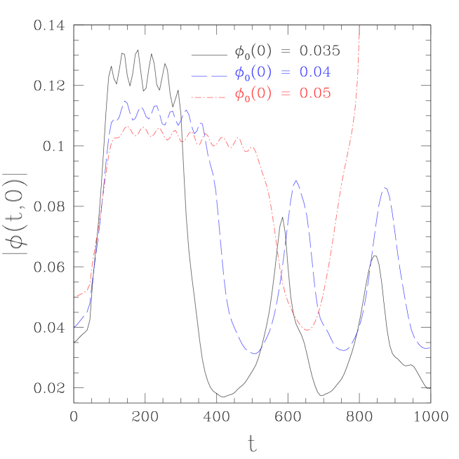
Figure 5: Time evolution of central value of the modulus of scalar field for subcritical evolution of perturbed boson stars. The figure shows the time evolution of $|\phi(t,0)|$ for marginally subcritical evolutions generated from boson star initial states with $\phi_{0}(0)=0.035,0.04$ and $0.05$. See the text for a description of key features of this plot.

Figure 6: Transition of perturbed boson stars in critical evolutions. The solid curve shows the parametric mass vs radius plot of static boson stars (curve parameter, $\phi_{0}(0)$), where we have defined the stellar radius, $R$, so that $M(R)=0.99\,M(\infty)=0.99\,M_{\rm ADM}$. Triangles label the initial configurations, squares show the corresponding critical solutions (identified as one-mode-unstable boson stars with oscillations—largely in fundamental mode), and the dashed arrows represent schematically the transition between the initial and critical states. See the text for more details.

The results from our simulations of critically perturbed boson stars are thus in agreement with previous studies [1, 2] that identified the critical states as excited (primarily in the first harmonic mode), unstable boson stars. Following that work we can display an approximate correspondence between the initial boson stars and the critical solutions as show in Fig. 6. The solid line shows the one-parameter family of static boson stars (parameterized as usual by $\phi_{0}(0)$), where we have defined the radius, $R$, of a boson star so that $M(R)=0.99M_{\rm ADM}=0.99M(\infty)$. The triangles indicate the initial stable boson star configurations, the squares indicate our best estimate of the corresponding unstable critical boson star states, and each arrow schematically depicts the transition between the two states that is induced by the perturbing scalar field. We note that to identify which unstable boson star is acting as the critical solution—which is equivalent to identifying an effective value of $\phi_{0}(0)$—we time average the central modulus of the complex field, $|\phi(t,0)|$ during the period of critical evolution. In addition, in accord with previous results, we observe that in all cases, the mass of the unstable critical state is larger than that of the progenitor boson star, indicating that a significant amount of mass-energy is extracted from the massless scalar field through its purely gravitational interaction with the complex field.

As discussed previously, for both subcritical and supercritical simulations, the closer one tunes $A_{3}$ to the critical value $A_{3}^{\star}$, the longer the perturbed star will persist in the critical state. Specifically, we observe scaling of the lifetime, $\tau$, of the critical evolution of the form

$$\tau(A_{3})\sim-\gamma\ln|A_{3}-A_{3}^{\star}|\,,$$ (111)

where we define the lifetime to be the lapse of coordinate time from the start of the evolution, $t=0$, to the time of first detection of an apparent horizon, and where $\gamma$ is a scaling exponent that depends on which of the infinitely many one-mode unstable boson stars acts as the critical solution in the particular scenario being simulated. We note that the details of the definition of $\tau$ are not important to the determination of $\gamma$ in (111) since $\gamma$ actually measures the differential in lifetime with respect to changes in $A_{3}-A_{3}^{\star}$, and this differential is insensitive to precisely how we define $\tau$, at least as $A_{3}\to A_{3}^{\star}$. In addition, we note that in using coordinate time in our definition of the scaling relationship (111), we are defining the scaling with respect to proper time at spatial infinity. Another choice—arguably more natural—would be to define $\tau$ in terms of the proper time measured by an observer at rest at $r=0$ (central proper time). Since the critical solutions are nearly static, the relation between these two different definitions of time would be a specific factor for each distinct value of $\phi_{0}(0)$, and would thus lead to a $\phi_{0}(0)$-dependent “renormalization” of the scaling exponents, $\gamma$.

Fig. 7 shows measured scaling laws from supercritical evolutions of perturbed boson stars defined by $\phi_{0}(0)=0.02,0.035,0.04$ and $0.05$. It is clear from these plots that, at least as $A_{3}\to A_{3}^{\star}$, we have lifetime scaling of the form (111). Estimated values of $\gamma$—computed from linear least-squares fits to the plotted data—are $\gamma=8.1,11,14,17$ for $\phi_{0}(0)=0.02,0.035,0.04,0.05$, respectively. We note that according to the now standard picture of critical collapse (see for example [29]), each value of $\gamma$ can be identified with the reciprocal Lyapunov exponent (i.e. growth factors) of the single unstable mode associated with the corresponding critical solution. Again, the reason that we observe different values of $\gamma$ for different choices of initial boson star (different values of $\phi_{0}(0)$) is that distinct critical solutions are being generated in the various cases. That is, we cannot expect universality (with respect to initial data) in this case because the model admits an entire family of one-mode unstable solutions that sit at the threshold of black hole formation.

Figure 7: Measured lifetime scaling laws for critically perturbed boson stars. This figure shows the measured lifetimes of various near-critical evolutions of perturbed boson stars as a function of $\ln|A_{3}-A_{3}^{\star}|$, for cases with $\phi(0)=0.02,0.035,0.04$ and $0.05$. Quoted scaling exponents, $\gamma$ (see (111) are computed from linear least-squares fits to the data. The apparent convergence of the data for different $\phi_{0}(0)$ as $\ln|A_{3}-A_{3}^{\star}|\to 0$ is not significant, as it reflects calculations far from criticality i.e. far from the $\ln|A_{3}-A_{3}^{\star}|\to-\infty$ limit. See the text for additional details.

0.17.3 Final Fate of Subcritical Evolutions

In previous work on the problem of critically perturbed spherically symmetric boson stars [1, 2], it was conjectured that the end state of subcritical evolution was characterized by dispersal of the boson star to large distances (relative to the size of the initial, stable star). This conjecture was at least partially influenced by the behaviour observed, for example, in the collapse of a massless scalar field [7], where subcritical evolutions do involve complete dispersal of the field. However, another key reason for what we claim is a misidentification of the true subcritical end-state was that the simulations described in [1, 2] simply were not carried out for sufficient coordinate time to see the long-time behaviour. Our current simulations strongly suggest that subcritical evolutions lead to a “relaxation” of the critically perturbed state to something that approximates a boson star (not necessarily the original star) undergoing large amplitude oscillations. As argued in the next sub-section, these oscillations can largely be identified with the fundamental perturbative mode associated with the final boson star state. The numerical evidence also suggests that these oscillating configurations eventually re-collapse in general; a “prompt” re-collapse can be seen in the $\phi_{0}(0)=0.05$ data in Fig. 5.

Fig. 8 shows the long-time behaviour of $\mbox{max}_{r}(2M(t,r)/r_{S})$, $|\phi(t,0)|$ and $\psi(t,0)$ for a near-critically perturbed boson star ($\phi_{0}(0)=0.04,A_{3}^{\star}\approx 0.00342$), where $r_{S}=\psi^{2}r$ is the areal radius, and where, loosely speaking, $2M(t,r)/r_{S}=1$ signals the surface of a black hole. Note that this is a subcritical evolution, so that a black hole does not form. As shown in more detail in previous figures, the boson star enters a critical state (well approximated by an unstable boson star) shortly after the real scalar field leaves the computational domain ($t\approx 100)$, and while in the critical state, it oscillates with the frequency of the fundamental mode as computed from perturbation theory using the unstable boson star state as the background (see [1, 2]). At $t\approx 370$ the star leaves the more compact critical configuration, decreases in central density, expands in size, and starts to pulsate with a different frequency. Although at late time the oscillation amplitudes are much larger than those seen in the critical phase of evolution, we will show in the following section that the oscillations can nonetheless be largely attributed to excitations of the fundamental perturbative mode associated with the final boson star state.

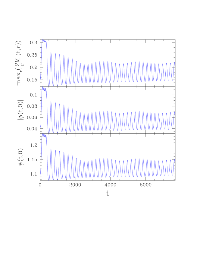
Figure 8: Long time behaviour of subcritical evolution for $\phi(0,0)=0.04$. This figure shows the long-time behaviour of $\max_{r}(2M(t,r)/r_{S})$, $|\phi(t,0)|$ and $\psi(t,0)$ for a near-critically perturbed boson star ($\phi_{0}(0)=0.04,A_{3}^{\star}\approx 0.00342$), where $r_{S}=\psi^{2}r$ is the areal radius, and where, loosely speaking, $2M(t,r)/r_{S}=1$ signals the surface of a black hole. Note that this is a subcritical evolution, so that a black hole does not form. The figure provides evidence that the final state of subcritical evolution is characterized by large amplitude oscillations about something approximating a boson star on the stable branch, rather than dispersal of the complex field as suggested in [1, 2]. Detailed calculation (see Sec. 0.17.4) shows that the pulsation frequency is approximately the fundamental mode frequency computed from perturbation theory about a background stable boson star solution with $\phi_{0}(0)=0.051$. Also note the overall lower-frequency modulation of the post-critical-phase oscillations. This effect is not yet understood, although one possible explanation—namely that the envelope modulation represents “beating” of the fundamental and first harmonic modes—appears to be ruled out.

0.17.4 Perturbation Analysis of Subcritical Oscillations

We now proceed to an application of perturbation theory to the oscillations seen in long-time evolutions of marginally subcritical configurations, such as those shown in Fig. 8. Here we follow [17] and [2], and refer the interested readers to those sources for details of the approach that are not included here. In particular, we emphasize that we have not carried out the complete perturbation analysis ourselves, but are simply using a computer code provided by Hawley [64] to analyze our current simulations. Nonetheless, to make contact between the perturbative and simulation results, it is useful to briefly review the setup of the perturbative problem.

To formulate the equations for the perturbation analysis, we first rewrite the complex scalar field as:

$$\phi(t,r)=\left(\psi_{1}(t,r)+i\psi_{2}(t,r)\right)e^{-i\omega t}\,,$$ (112)

(Note that this representation is distinct from $\phi=\phi_{1}+i\phi_{2}$, and the reader should be careful not to confuse the $\psi$’s used here with the conformal metric variable, $\psi$.) Additionally, the spacetime metric is written in Schwarzschild-like (polar-areal) coordinates:

$$ds^{2}=-e^{\nu(t,r)}dt^{2}+e^{\lambda(t,r)}dr^{2}+r^{2}\left(d\theta^{2}+\sin^{2}\theta d\varphi^{2}\right)\,.$$ (113)

We further introduce four perturbation fields $\delta\lambda(t,r),\delta\nu(t,r),\delta\psi_{1}(t,r)$ and $\delta\psi_{2}(t,r)$ which represent the perturbations about the equilibrium values $\lambda_{0}(r),\nu_{0}(r),\phi_{0}(r)$:

$$\lambda(t,r) = \lambda_{0}(r)+\delta\lambda(t,r)\,,$$ (114)

$$\nu(t,r) = \nu_{0}(r)+\delta\nu(t,r)\,,$$ (115)

$$\psi_{1}(t,r) = \phi_{0}(r)\left(1+\delta\psi_{1}(t,r)\right)\,,$$ (116)

$$\psi_{2}(t,r) = \phi_{0}(r)\,\delta\psi_{2}(t,r)\,.$$ (117)

With the above definitions we can write the coupled Einstein-Klein-Gordon field equations as a set of PDEs for the functions $\delta\lambda,\delta\nu,\delta\psi_{1}$ and $\delta\psi_{2}$. With some manipulation we can then eliminate $\delta\nu$ and $\delta\psi_{2}$ to produce a system of two coupled second-order PDEs for $\delta\psi_{1}$ and $\delta\lambda$:

$$\delta{\psi_{1}}^{\prime\prime} = -\left(\frac{2}{r}+\frac{{\nu_{0}}^{\prime}-{\lambda_{0}}^{\prime}}{2}\right)\delta{\psi_{1}}^{\prime}-\frac{\delta\lambda^{\prime}}{r{\phi_{0}}^{2}}+e^{\lambda_{0}-\nu_{0}}\ddot{\delta\psi_{1}}$$ (118)

$$-\left[\frac{{\phi_{0}}^{\prime}}{\phi_{0}}\left(\frac{{\nu_{0}}^{\prime}-{\lambda_{0}}^{\prime}}{2}+\frac{1}{r}\right)+\left(\frac{{\phi_{0}}^{\prime}}{\phi_{0}}\right)^{2}+\frac{1-r{\lambda_{0}}^{\prime}}{r^{2}{\phi_{0}}^{2}}+e^{\lambda_{0}-\nu_{0}}\omega^{2}-e^{\lambda_{0}}\right]\delta\lambda$$

$$+2e^{\lambda_{0}}\left[1+e^{-\nu_{0}}\omega^{2}+e^{-\lambda_{0}}\left(\frac{{\phi_{0}}^{\prime}}{\phi_{0}}\right)^{2}+r\phi_{0}{\phi_{0}}^{\prime}\right]\delta\psi_{1}\,,$$

$$\delta\lambda^{\prime\prime} = -\frac{3}{2}\left({\nu_{0}}^{\prime}-{\lambda_{0}}^{\prime}\right)\delta\lambda^{\prime}+\left[4{{\phi_{0}}^{\prime}}^{2}+{\lambda_{0}}^{\prime\prime}+\frac{2}{r^{2}}-\frac{({\nu_{0}}^{\prime}-{\lambda_{0}}^{\prime})^{2}}{2}-\frac{2{\nu_{0}}^{\prime}+{\lambda_{0}}^{\prime}}{r}\right]\delta\lambda$$ (119)

$$+e^{\nu_{0}-\nu_{0}}\ddot{\delta\lambda}-4\left(2\phi_{0}{\phi_{0}}^{\prime}-re^{\lambda_{0}}{\phi_{0}}^{2}\right)\delta{\psi_{1}}^{\prime}$$

$$-4\left[2{{\phi_{0}}^{\prime}}^{2}-re^{\lambda_{0}}{\phi_{0}}^{2}\left(2\frac{{\phi_{0}}^{\prime}}{\phi_{0}}+\frac{2{\nu_{0}}^{\prime}+{\lambda_{0}}^{\prime}}{2}\right)\right]\delta\psi_{1}\,.$$

Note that these equations involve only second time derivatives (i.e. there are no terms involving $\dot{\delta\psi_{1}}$ or $\dot{\delta\lambda}$), and that they are linear in the second time derivatives. If we thus assume a harmonic time-dependence for the perturbed fields:

$$\delta\psi_{1}(t,r) = \delta\psi_{1}(r)e^{i\sigma t}\,,$$ (120)

$$\delta\lambda_{1}(t,r) = \delta\lambda_{1}(r)e^{i\sigma t}\,,$$ (121)

then the equations for the perturbations contain $\sigma$ only in the form $\sigma^{2}$, and the sign of $\sigma^{2}$, as computed by solving a particular mode equation, determines the stability of that mode. (Note that the system can be shown to be self-adjoint so that the values of $\sigma^{2}$ must be real.) If any of the values of $\sigma^{2}$ are found to be negative, then the associated perturbations will grow and the boson star will be unstable. Moreover, as the eigenvalues form an infinite discrete ordered sequence, examining the fundamental radial mode ${\sigma_{0}}^{2}$ determines the overall stability of any particular star with respect to radial perturbations.

In order to compare the simulation results with those given by perturbation theory, we first observe that there is a difference in the choice of the time coordinates used in the two calculations. Specifically, in the perturbative analysis [17, 2], the lapse was chosen to be unity at the origin, so we have

$$\sigma^{2}\Bigl{.}\Bigr{|}_{\rm perturbative}\rightarrow{\sigma^{2}\over\alpha^{2}}\Bigl{.}\Bigr{|}_{\rm simulation}\,.$$

We also note that there is a factor of 2 difference in the definitions of $T_{\mu\nu}$ used in the two calculations, and that the definition of the complex field, $\phi(t,r)$, in the perturbative calculation includes a factor of $\sqrt{8\pi}$. We thus have

$$\phi\Bigl{.}\Bigr{|}_{\rm perturbative}\rightarrow\sqrt{4\pi}\phi\Bigl{.}\Bigr{|}_{\rm simulation}\,.$$

The numerical technique for obtaining the fundamental mode and first harmonic mode frequencies of boson stars has already been described in [2] and will not be repeated here; again we will simply quote and use results from that study. From Fig. 8 we note that there are 20 oscillations between $t=620$ and $t=5200$, giving a period $T\approx 229$. Hence we have an oscillation frequency $\sigma=2\pi/T\approx 0.0274$. The time average of the lapse function $\langle\alpha(t,0)\rangle$ in the interval is 0.78, and so $\sigma^{2}/\alpha^{2}\approx 0.0013$. We also compute the time average of $\phi(t,0)$ in the interval, and use the resulting value to identify the stable boson star solution about which we perform the perturbation analysis. We find $\langle\phi_{0}(t,0)\rangle\approx 0.051\times\sqrt{4\pi}=0.18$. For a boson star with $\phi_{0}(0)=0.18$, the perturbative calculations (see Fig. 7 of [2]) predict $\sigma_{0}^{2}=0.0014$, which is in reasonable agreement with the simulation results. Hence the oscillations that occur in the post-critical regime appear to be largely fundamental mode oscillations of a final-state, stable, boson star. We also remark that since the oscillations are of such large amplitude, it does not appear possible to precisely identify an effective background state (i.e. an effective value of $\phi_{0}(0)$), so the level of agreement in the oscillation frequencies is possibly as good as one could expect.

We have also attempted to understand the nature of the slower frequency oscillation which modulates the envelope of the fundamental-mode oscillations, as is visible in Fig. 8. One hypothesis is that this modulation represents a “beating” effect of two oscillatory modes with frequencies $\sigma_{1}$ and $\sigma_{2}$ such that $|\sigma_{1}-\sigma_{2}|\ll\sigma_{1,2}$. We observe that period of the envelope of oscillation is roughly $T\approx 2000$, corresponding to a squared-frequency $\sigma=2\pi/T\approx 0.00314$. The average of the lapse function during one cycle is roughly 0.78, so $\sigma^{2}/\alpha^{2}\approx 1.62\times 10^{-5}$. However, the first harmonic frequency from perturbation analysis for $\langle\phi_{0}(t,0)\rangle\approx 0.18$ is $\sigma_{1}^{2}=0.0105$, much different from the fundamental mode $\sigma_{0}^{2}=0.0014$. Therefore the beating cannot be produced from the superposition of the fundamental and first harmonic modes.

0.18 Black Hole Excision for Boson Stars

In the last section of this chapter we describe our application of black hole excision techniques in the context of gravitational collapse of boson stars. As described in Chap. A Numerical Study of Boson Stars, black hole excision methods, whereby the interiors of black holes are excluded from the computational domain, have been the subject of intense study in numerical relativity over the past decade. We view our current implementation as a further proof-of-principle for the strategy, as well as providing some indications of the subtle interactions between inner (excision) and outer boundaries that can arise when using the excision method. We also emphasize that we have not yet used calculations with excision in order to generate new results of physical significance.

To study excision techniques, we naturally need to evolve spacetimes which eventually develop black holes. Conveniently, we can consider the same model and initial data configurations used in our previously-described study of critical phenomena, provided that a sufficiently large amplitude factor, $A_{3}$, for the scalar field is used. In particular, we need to choose $A_{3}$ large enough so that the black hole that forms is large compared to the spatial discretization scale, $\Delta r$, used in the simulation. For the purposes of illustrating our implementation of excision, we consider a boson star with $\phi_{0}(0)=0.01$, and perturb it with an imploding massless scalar field having an initial profile of the form (109) with $A_{3}=0.041$, $r_{0}=40$ and $\sigma=5$. In fact, $A_{3}$ is large enough in this instance that almost all of the mass associated with both the real and complex fields ends up in the final black hole.

Fig. 9 shows a series of snapshots of $2M(t,r)/r_{S}$ during the resulting evolution, where $M(t,r)$ is the mass aspect function and $r_{S}=\psi^{2}r$ is the areal coordinate ($r$ is the isotropic radial coordinate). During the evolution we monitor (22) to detect the appearance of an apparent horizon—in this case an apparent horizon is first detected at $t=80.51$ and at $r=9.67$. Assuming cosmic censorship, the region $r\leq 9.67$ lies within a black hole for all future times so can safely be excised from the simulation domain for $t\geq 80.51$. (In Fig. 9, the region being excised lies to the left of the dashed vertical line in each sub-plot.) Fig. 10 shows the relative time rate of change of the mass aspect function at outer boundary, $\partial_{t}M(t,r_{\rm max})/M(t,r_{\rm max})$, for the same evolution. At late time ($t>100$) the relative change in the mass aspect function at outer boundary is of the order of $10^{-6}$, indicating almost no mass is passing through the outer boundary.

Figure 9: Evolution of a highly perturbed boson star ($\phi_{0}(0)=0.01$) using black hole excision. This figure shows snapshots of $2M(t,r)/r_{S}$, where $r_{S}=\psi^{2}r$ is the areal radius, and where, loosely speaking, $2M(t,r)/r_{S}=1$ signals the surface of a black hole. In snapshots with a vertical dashed line, the region from $r=0$ to the radial position of the dashed line is excised from the computational domain. The evolution starts with a stable boson star centered at the origin, and a high-amplitude, in-going pulse of real scalar field of the form (109) ($A_{3}=0.041$, $\sigma=5$ and $r=40$). At $t\approx 80$ the real field reaches the origin, and an apparent horizon containing most of the combined mass of the real and complex scalar fields forms at $t=80.51$. At late times, the exterior solution settles down to a configuration very close to a static Schwarzschild spacetime. Note that the temporal spacing between successive snapshots is not constant–the time instants displayed have been chosen to illustrate the key features of the simulation.

Figure 10: Relative time rate of change of the mass aspect function at outer boundary, $\partial_{t}M(t,r_{\rm max})/M(t,r_{\rm max})$, for the evolution of a highly perturbed boson star ($\phi_{0}(0)=0.01$) using black hole excision. The figure shows the result for the same evolution in Fig. 9, with $r_{\rm max}=150$ and $\Delta r\approx 0.146$. At late time $t>100$ the relative change in the mass aspect function at outer boundary is of the order of $10^{-6}$, indicating almost no mass is passing through the outer boundary.

Once excision is enabled, the origin is no longer part of the computational domain and thus the inner boundary (regularity) conditions previously imposed at $r=0$ for the variables $\alpha,\psi$ and $K^{r}{}_{r}$, must be replaced by conditions imposed at the excision surface. In the case of the dynamical geometrical variables, $\psi$ and $K^{r}{}_{r}$, we can use discrete versions of the evolution equations (23) and (24) to update values for $\psi$ and $K^{r}{}_{r}$ on the excision boundary. For the case of the lapse function, $\alpha$, we have found that a simple strategy, whereby we ‘freeze” the inner value of the lapse to whatever its value is when excision starts, leads to stable, convergent results. (Also note that since our simulations do appear to converge using our simple strategy, we have not experimented with the condition on $\alpha(r_{e},t)$, where $r_{e}$ is the $r$-coordinate of the excision surface. So, for example, we have not investigated whether the condition on $\alpha$ is perturbatively stable.) Finally, although the shift component, $\beta$, also satisfies a regularity condition, the boundary condition for (49), which governs the shift, is naturally set at large $r$ and thus we do not need to specify a condition on $\beta$ at the excision surface.

With regards to our simulations with excision, a key observation is that after the coupled boson star/real scalar field configuration promptly collapses to form a black hole, the region exterior to the black hole quickly settles down to an essentially Schwarzschild spacetime. In particular, the mass aspect function outside the black hole approaches an almost-constant function, and a stable simulation of the black hole spacetime can be carried out for very long integration times.

However promising the excision technique appears, careful examination of the mass aspect function over sufficiently long integration times does reveal certain numerical artifacts. For example, Fig. 11 plots the mass aspect function at the outer boundary of the computational domain, $r=r_{\rm max}=150$, against time, for $0\leq t\leq 360$. During any period where there is no flux of real or complex mass/energy crossing the outer boundary, we should have $M(t,r_{\rm max})={\rm const.}$ From the figure we see that $M(t,r_{\rm max})$ decreases initially, mainly due to the escape of real scalar field from the computational domain. At $t\approx 80$, following the first detection of an apparent horizon, and the enabling of excision, there is a relatively sharp, and transient decrease in $M(t,r_{\rm max})$. However, as can also be seen in the figure, all indications are that this particular decrease “converges away” in the continuum limit $\Delta r\to 0$. Following the transient phase, although the mass generically remains roughly constant, there is always a small rate of increase in $M(t,r_{\rm max})$ which is largely independent of the grid resolution, $\Delta r$. This is surely an artifact—since no mass is physically added to the system, we claim that the observed mass increase must be a purely numerical/computational effect, and we have thus investigated possible remedies.

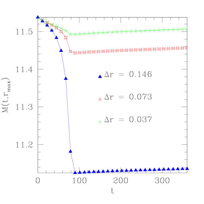
Figure 11: The mass aspect function $M(t,r_{\rm max})$ vs $t$ for $r_{\rm max}=150$ from simulations with excision, and computed using three different finite difference resolutions, $\Delta r$, in a 4:2:1 ratio. For resolution $\Delta r=0.146$, (the coarse calculation), the mass decreases quite suddenly (and by a few percent) at $t\approx 80$, at which time a black hole is detected and a region of spacetime is excised. Following this early transient associated with the enabling of excision, the mass remains roughly constant (relative to the transient fluctuation), although a slight constant rate of mass increase is observed. As resolution increases ($\Delta r=0.073$, $\Delta r=0.037$), the early transient mass decrease apparently converges away (possibly only as $\Delta r$). However, the late-time mass increase, does not seem to vanish as $\Delta r\to 0$ as can be seen from the fact that the slope of the plots for $t>100$ remains roughly constant as the resolution is varied.

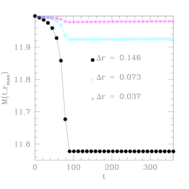
Figure 12: The mass aspect function $M(t,r_{\rm max})$ vs $t$ for $r_{\rm max}=300$ from simulations with excision, and computed using three different finite difference resolutions, $\Delta r$, in a 4:2:1 ratio. As in Fig. 11, with increasing resolution, the magnitude of the early ($t\approx 80$) transient mass drop apparently converges away. Moreover, the mass is more nearly conserved at late times in the calculation, relative to the simulation shown in Fig. 11. In other words, the spurious mass increase seems to be due to our treatment of the outer boundary conditions, and we can apparently suppress the resulting numerical artifacts by increasing the size of the computational domain.

Because our simulations are performed on a finite radial domain, $0\leq r\leq r_{\rm max}$, it is natural to consider the effect of the placement of the outer boundary of the domain, $r_{\rm max}$, on the results. Fig. 12 plots $M(t,r_{\rm max})$ vs $t$ from simulations using the same initial data described in Fig. 11, but where $r_{\rm max}$ has been doubled to $r_{\rm max}=300$. From this figure it can be seen that the transient mass decrease immediately following the enabling of excision still converges away as $\Delta r\to 0$. In addition, it is apparent that the level of mass increase following the transient phase is substantially reduced from the $r_{\rm max}=150$ calculations. To illustrate this point more clearly, Fig. 13 shows the deviation of the mass aspect function $M(t,r_{\max})$ from $M(190,r_{\max})$ vs time $t$ for $r_{\max}=150,300$ and $600$. The deviation is measured relative to the mass aspect function at $t=190$, by which time the transients associated with the enabling of excision have settled down. The figure shows that the deviation is smaller when we increase the location of the outer boundary from $r_{\max}=150$ to $r_{\max}=300$ and $r_{\max}=600$. The calculated value for $\left(\Delta M(t,150)-\Delta M(t,300)\right)/\left(\Delta M(t,300)-\Delta M(t,600)\right)\approx 5$, where $\Delta M(t,r_{\max})\equiv M(t,r_{\max})-M(190,r_{\max})$, which indicates the rate of convergence is roughly $r_{\max}^{-2}$.

We thus conjecture that the most dominant contribution to the small amount of post-excision “mass inflation” we observe is due to our (approximate) asymptotic treatment of the boundary conditions. We have done some preliminary investigations of improvements to the outer boundary conditions but have no significant findings to report at this time.

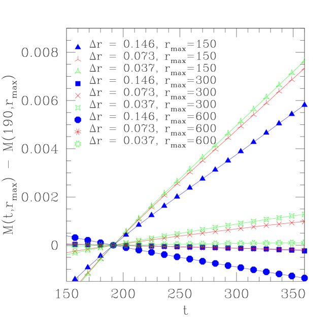
Figure 13: The deviation of the mass aspect function $M(t,r_{\rm max})$ from $M(190,r_{\rm max})$ vs $t$ for $r_{\rm max}=150,300$ and $600$ from simulations with excision, and computed using three different finite difference resolutions, $\Delta r$, in a 4:2:1 ratio. The deviation is measured relative to the mass aspect function at $t=190$, by which time the transients associated with the enabling of excision have settled down (see Fig. 11 and Fig. 12). The deviation is smaller when we increase the location of the outer boundary from $r_{\max}=150$ to $r_{\max}=300$ and $r_{\max}=600$. The rate of convergence is roughly $r_{\rm max}^{-2}$. See the text for further details.

Chapter 0 Boson Stars in Axisymmetry

We now consider the evolution of the coupled Einstein-Klein-Gordon field equations in axisymmetry. As time-dependent, spherically symmetric spacetime is the most natural 1 space + 1 time-dimensional arena in which to approximate star-like objects, so is time-dependent axisymmetric spacetime the most natural 2+1 context. Crucially, the generalization to axisymmetry allows us to consider time-independent configurations with net angular momentum, which, for the case of boson stars turn out to be surprisingly non-trivial to construct. In addition, with an axisymmetric code we can simulate scenarios such as the head-on collision of two or more boson stars, as well as axisymmetric (i.e. non-spherically symmetric) critical collapse. This chapter concerns the construction of stationary (time-independent ), rotating boson star solutions (which requires the solution of an elliptic quadratic eigenvalue problem in two spatial dimensions), as well as the construction of time-dependent axisymmetric solutions representing the evolution of generic (in principle) axisymmetric initial data for a complex scalar field. Unfortunately, the stationary solutions that we construct in the first case are not time-independent in the coordinate system used in the latter  and we are thus unable to directly study the evolution of rotating boson stars by combining the two calculations. We are, however, able to reproduce and extend previous calculations of rotating boson star configurations, as well as to study critical collapse of driven boson stars in axisymmetry through a completely original set of calculations. Some of the work presented in this chapter was done in collaboration with Choi [75], who performed numerous tests on the solutions for stationary rotating boson stars in the Newtonian limit, as well as tests of the modified graxi code. Results of these tests are available on-line [75] and will not be further described here.

Before proceeding to a summary of the remainder of the chapter, we present an overview of some key features of general relativistic, rotating boson stars (and previous work on the subject), and then an overview of related work on axisymmetric critical collapse as well as our general approach to that problem.

0.18.1 Rotating Boson Stars

The question of existence of rotating fluid stars (solutions of the stationary, axisymmetric Einstein/hydrodynamics equations) has a clear answer on physical grounds. The observation of rotating neutron stars—for example, in the form of pulsars—tells us that relativistic, rotating fluid stars naturally occur in our universe, and the theoretical study of such objects has been an active area of research for decades (for example, see [22, 76, 77, 78, 79, 80]). Interestingly, it was not until fairly recently that the theoretical existence of relativistic, rotating boson stars was demonstrated [26, 28, 81]. This is perhaps not too surprising when one considers the lack of astrophysical importance (to date at least!) of boson stars. In addition, at a more technical level, the regularity condition for a rotating bosonic star is different from that for a rotating fermionic star, a fact which leads to completely different topological shapes for the rotating stationary states in the two cases. For example, as has already been mentioned, for boson stars with non-zero angular momentum, the stationary solutions have mass-energy concentrated in a roughly toroidal (rather than spheroidal) configuration.

Schunck & Mielke [26], as well as Yoshida & Eriguchi [28] have previously constructed general relativistic, stationary, rotating boson star solutions using numerical means. One of the more interesting features of such solutions is that angular momentum is quantized (or perhaps more properly, discretized). Specifically, to generate time-independent, rotating configurations, one is naturally lead to an ansatz (in spherical-polar coordinates) 

$$\phi(t,r,\theta,\varphi)\longrightarrow\phi_{0}(r,\theta)e^{i\omega t+ik\varphi}\,.$$ (1)

Now, $\omega$ can in principle take on arbitrary real values; $k$, however, must be integral for $\phi$ to be single valued. Since the specific choice of $k$ affects boundary conditions at $r=0$, the ansatz (1) itself naturally leads us to consider a series of (elliptic eigenvalue) problems for $k=1,2,\cdots$ (the case $k=0$ describes the spherical boson stars of Chap. A Numerical Study of Boson Stars).

As in the spherical case, $k=0$, for any value of $k=1,2,\cdots$, $\omega$ will be the eigenvalue $\omega({\phi_{(k)}})$, where ${\phi_{(k)}}$, is a generalization of the central modulus value, $\phi_{0}$, conventionally used to parametrize the family of stars in spherical symmetry. In other words, as was the case in spherical symmetry, for each value of the angular momentum parameter (or azimuthal quantum number), $k$, we expect to find an entire family of rotating stars, which will be parametrized by ${\phi_{(k)}}$.

Given the clear analogy between (1) and axisymmetric bound states in quantum mechanics, it is perhaps not surprising that rotating boson stars have distinctive topological characteristics. In fact, given the ansatz (1) one can show that regularity as $r\to 0$ implies

$$\lim_{r\to 0}\phi_{0}(r,\theta;k)=r^{k}f_{k}(\theta)+O(r^{k+2})\,.$$ (2)

Thus, for $k>0$ (i.e. the non-spherically symmetric cases) we have that $\phi$ and its first $k-1$ radial derivatives vanish on axis, and are relatively small close to the axis. This means that for $k\geq 1$, the boson stars might be more accurately termed boson tori.

Solutions for rotating boson stars using the full general relativistic equations were first obtained by Schunck & Mielke [26, 81]. Specifically, configurations for $2\leq k\leq 10$ as well as for $k=500$ were found. However, as pointed out by Yoshida & Eriguchi [28] the solutions obtained were all close to Newtonian; for instance, in [81] a $k=1$ solution is presented which has $M=0.07331M_{{\rm pl}}^{2}/m$, a mass that is only about 6% of the maximum possible mass for the $k=1$ family. Overall we estimate that none of the solutions constructed by Schunck & Mielke (for any of the values of $k$ considered) have masses in excess of 10% of the maximum mass of the corresponding family. As another example of the weak-field nature of the Schunck & Mielke solutions, the quasi-Newtonian potentials that are displayed have almost no angular dependence, whereas the potentials corresponding to highly relativistic stars do. Moreover, Schunck & Mielke determined only a few configurations for any value of $k$, and thus did not study any specific family of solutions in sufficient detail to determine, for example, whether a “Chandrasekhar limit” existed, as is the case for fluid stars, as well as for spherically symmetric boson stars. Finally, some of the solution plots in [26] (such as Figs. 6.4 and 6.6) are not very smooth, indicating that the calculations may have been underresolved.

The work by Yoshida & Eriguchi [28] represented a significant advance over Schunck & Mielke’s in several respects. The solutions they constructed were smooth, and they were able to compute the entire family of solutions for the case $k=1$. Further, they showed that the plot of $M^{k=1}_{\rm ADM}({\phi_{(k)}})$ (where ${\phi_{(k)}}$ is again the family parameter), exhibited a maximum, and concluded that the maximum mass for a $k=1$ rotating boson star is $M_{\rm max}=1.31M_{{\rm pl}}^{2}/m$.

Despite the considerable success of the calculations described in [28], we have identified several unsatisfactory points about that work as well, and have at least partially ameliorated the identified weaknesses in our current research. First, the code used in [28] breaks down before the maximum-mass star for $k=2$ can be computed, whereas the method we describe below can be used to compute the complete family for the $k=2$ case. Second, Yoshida & Eriguchi’s numerical approach uses a so-called “self-consistent field” method in which the solutions are represented as two-dimensional surface integrals at every mesh point (the mesh itself is two-dimensional); this means the solution algorithm is quite expensive. In contrast, we adopt a finite-difference approach that uses homotopic and multigrid techniques to solve the resulting non-linear, elliptic eigenvalue problem, and although we have no way of performing direct timing estimates, we feel that our approach is likely to be significantly more efficient computationally.

Finally, although our calculations are currently limited by regularity problems (so that, for example, we cannot compute solutions for $k=3,4,\cdots$), we have reformulated our basic equations in a manner that we feel will largely solve those problems (see Sec. 0.20.6). Although work on the modification of our algorithm to solve this new system is not complete, we feel that with it we will be able to compute families of solutions for $k>2$, and, importantly, will be able to do proper convergence tests to assess the accuracy of the results. The lack of convergence tests or other means of estimating the accuracy of solutions is another shortcoming of both the Schunck & Mielke and Yoshida & Eriguchi work, and, indeed, our regularity problems inhibit the complete convergence testing of our current results as well. We note that regularity problems near coordinate singularities in curvilinear coordinates have often been encountered in calculation in numerical relativity. In this case, we have no rigorous understanding of the origin of these problems; however, we have strong evidence that the solutions of the discrete equations are not regular as $r\to 0$ (i.e. our solution of the non-linear eigenvalue problem is currently unstable).

0.18.2 Axisymmetric Critical Phenomena

An investigation of axisymmetric critical phenomena very similar to the one described below was carried out by Rousseau [31], who studied critical phenomena associated with driven collapse of spherically symmetric boson stars in the context of the so-called conformally flat (or Isenberg-Mathews-Wilson) approximation to general relativity. Using a massless scalar field as the perturbing agent, Rousseau was able to verify the existence of families of solutions that interpolate across the black hole threshold (the conformally flat approximation admits solutions with apparent horizons), and found some evidence of Type I behaviour—with the critical solutions being unstable boson stars—and indications of lifetime scaling of the form (45). However, Rousseau’s calculations were not fully relativistic, and were severely resolution-limited, so the results are neither very complete nor accurate.

All of the dynamical studies described below have been performed using a code, graxi, previously developed by Choptuik, Hirschmann Liebling & Pretorius [8, 9], that solves the coupled Einstein-Klein-Gordon equations in axisymmetry. I was responsible for the implementation of the initial data interface for boson stars, as well as for the execution and analysis of the numerical experiments reported in this Chapter. We note that the dynamical calculations that we describe in Sec. 0.21 are quite well resolved and accurate (estimated local accuracy of a few percent) by virtue of the fact that graxi incorporates Berger-and-Oliger-style adaptive mesh refinement.

We have used graxi to investigate Type I critical behaviour of axisymmetric boson stars using two novel strategies. The first involves the head-on collision of two identical spherically symmetric boson stars, where the family parameter is the initial momentum, $p_{z}$, imparted to each star. The second involves perturbation of a single spherically symmetric boson star via the implosion of a non-spherically-symmetric pulse of massless scalar radiation. In this case the family parameter is the overall amplitude of the initial massless scalar pulse. In both instances we find strong evidence for Type I behaviour, as well as strong evidence for lifetime scaling of the form (45). In addition, in some of the collision simulations we observe interesting “solitonic” behaviour that has previously been seen in the collision of Newtonian boson stars [32].

0.18.3 Outline

The remainder of this chapter is organized as follows. We start in Sec. 0.19 with a review of the most general geometrical notion of “time-independence” for a generic spacetime (stationarity) and a discussion of a suitably general, symmetry-adapted coordinate system in which to study axisymmetric, stationary solutions of the coupled Einstein-Klein-Gordon equations. We then proceed in Sec. 0.20 to a discussion of an approach to the construction of solutions representing general relativistic stationary boson stars with angular momentum. As with the determination of spherical boson star data per se, this involves the solution of the initial value (constraint) equations for the gravitational field, but is significantly complicated by the fact that we must simultaneously solve a non-linear elliptic eigenvalue problem (an elliptic PDE) for the matter field. In contrast to the previous work of Yoshida & Eriguchi [28], which employed a so-called “self-consistent field” technique, we proceed via finite-difference solution of the stationary PDEs for rotating boson stars and outline some of the computational challenges that result in Sec. 0.20.2. In Sec. 0.20.3 we then discuss details of the multigrid-based solver that we have designed and implemented to solve the eigenvalue problem. Results for rotating boson stars generated using the solver are presented in Sec. 0.20.4 and we follow with remarks concerning the performance of our method and possible enhancements in Sec. 0.20.5.

As already mentioned, our solver for rotating boson stars is currently limited by regularity problems, and we are, in fact, unable to compute solutions for $k=3,4,\cdots$. One promising approach to resolving this difficulty is to redefine variables (both scalar field and geometric) so that regularity in the discrete domain is more automatically enforced. To that end we present a candidate reformulation of the equations in Sec. 0.20.6. Although we have not yet implemented a solver for a discretization of this new system, we are confident that this task will be straightforward, given the computational techniques that we have already developed. We thus hope that the incomplete work described in Sec. 0.20.6 will soon give rise to a solver that will work for $k>2$.

In Sec. 0.21 we turn attention to the dynamics of boson stars. We discuss the results from a study of head-on collisions of two boson stars in Sec. 0.21.2 and finally, in Sec. 0.21.5, we summarize results from axisymmetric generalizations of the spherical critical collapse studies previously described in Sec. 0.17.

0.19 Stationary, Axisymmetric Spacetime

As mentioned above, the concept of stationarity in general relativity is meant to capture the most general geometric notion of “time-independence”. A spacetime is stationary if it admits a timelike Killing vector field, and operationally, we will equivalently define a stationary spacetime as one for which, at least locally, there exists a coordinate system in which all metric components are independent of the time coordinate, $t$.  In addition, we now wish to restrict attention to axisymmetric spacetimes, so that the spacetime also has a spacelike, azimuthal Killing vector (with closed orbits). Again, we will assume that this means that we can choose a coordinate system with one of the coordinates, $\varphi$, adapted to the symmetry, so that none of the metric coefficients in that coordinate system depend on $\varphi$. In other words, for stationary, axisymmetric spacetimes, if we adopt “natural” (i.e. symmetry-adapted) spherical-polar coordinates, $(t,r,\theta,\varphi)$, the metric will depend only on $r$ and $\theta$:

$$g_{\mu\nu}(t,r,\theta,\phi)\longrightarrow g_{\mu\nu}(r,\theta)\,\,.$$

Since we are considering rotating configurations, our spacetimes will in general not exhibit time reversal symmetry as $t\to-t$ will result in a configuration representing stars rotating in a sense opposite to the original. (In other words, stationary spacetimes are not necessarily static.) However, our spacetimes should be invariant if we simultaneously reverse both time and the azimuthal angle, i.e. the metric should have the discrete symmetry $(t,\varphi)\rightarrow(-t,-\varphi)$. In the general expression for the line-element in symmetry-adapted coordinates this fact immediately excludes the $dtdr$, $dtd\theta$, $drd\varphi$ and $d\theta d\varphi$ terms as they do not preserve this discrete symmetry. Finally, we can perform a coordinate transformation [82] such that the metric of the 2-dimensional $r$-$\theta$ subspace has the diagonal form

$$\psi^{4}\left(dr^{2}+r^{2}d\theta^{2}\right)\,,$$

as long as the subspace has a positive-definite (or negative-definite) signature. With these considerations we can now write a suitably general form for the metric of a stationary, axisymmetric spacetime:

$$ds^{2}=-\alpha^{2}dt^{2}+u\left(\beta dt+d\varphi\right)^{2}+\psi^{4}\left(dr^{2}+r^{2}d\theta^{2}\right)\,.$$ (3)

To summarize, by an appropriate choice of coordinates, we can reduce the number of non-trivial metric components that are needed to describe stationary, axisymmetric spacetimes to four; here we identify those four quantities with the functions $\alpha,\beta,\psi$ and $u$. In what follows, we will also restrict attention to those stationary, axisymmetric configurations with equatorial symmetry (i.e. those that are symmetric under $\theta\to\pi-\theta$). We thus can compute using the reduced angular range $0\leq\theta\leq\pi/2$.

0.20 The Initial Value Problem for Rotating Boson Stars

0.20.1 The System of Equations in Quasi-Isotropic Coordinates (System A)

Paralleling what was done in the case of spherical symmetry in the previous chapter, we have adopted what we will call the quasi-isotropic (spatial) coordinate condition in choosing the form (3) for the metric of a general axisymmetric, stationary spacetime. In fact, it is convenient to take $u$ in (3) to be of the form

$$u\equiv\psi^{4}r^{2}\sin^{2}\theta e^{2\sigma}\,,$$ (4)

so that the deviation of $\sigma(r,\theta)$ from zero reflects the deviation of the 3-metric from conformal flatness. Thus, the spacetime metric now becomes

$$ds^{2}=-\alpha^{2}dt^{2}+\psi^{4}r^{2}\sin^{2}\theta e^{2\sigma}\left(\beta dt+d\varphi\right)^{2}+\psi^{4}\left(dr^{2}+r^{2}d\theta^{2}\right)\,,$$ (5)

or

$$ds^{2}=\left(-\alpha^{2}+\psi^{4}r^{2}\sin^{2}\theta e^{2\sigma}\beta^{2}\right)dt^{2}+\psi^{4}\left(dr^{2}+r^{2}d\theta^{2}+r^{2}\sin^{2}\theta e^{2\sigma}d\varphi^{2}\right)+2\psi^{4}r^{2}\sin^{2}\theta e^{2\sigma}\beta dtd\varphi$$ (6)

where, again, $\alpha,\beta,\psi$ and $\sigma$ are functions of $r,\theta$ only. To generate stationary solutions (having angular momentum in general) we adopt the following ansatz for $\phi(t,r,\theta,\varphi)$:

$$\phi(t,r,\theta,\varphi)=\phi_{0}(r,\theta)e^{-i(\omega t+k\varphi)}\,.$$ (7)

As discussed above, and is the case for a quantum mechanical wave function, $k$ must take on integer values, since $\phi$ must be single valued with respect to $\varphi$:

$$\phi(t,r,\theta,\varphi)=\phi(t,r,\theta,\varphi+2\pi)\,.$$ (8)

As we have also previously remarked, this “quantization” of angular momentum is one of the more novel features of rotating boson star solutions relative to rotating fluid configurations.

We can now proceed to derive the PDEs for stationary boson stars in quasi-isotropic coordinates from the Hamiltonian and momentum constraints, the Klein-Gordon equation, the ansatz (7), and the assumption of stationarity. Since the derivation is lengthy but straightforward, we will simply state the resulting equations. For numerical convenience we choose $\kappa=1$ instead of the usual convention $\kappa=8\pi$ (see (1)) as in the previous chapter.

First, from the Klein-Gordon equation we have the following

$$\begin{split}\phi_{,rr}+\frac{2}{r}\phi_{,r}+\frac{1}{r^{2}}\phi_{,\theta\theta}+\frac{\cot\theta}{r^{2}}\phi_{,\theta}-\frac{k^{2}}{r^{2}\sin^{2}\theta e^{2\sigma}}\phi+\left(\sigma_{,r}+\frac{\alpha_{,r}}{\alpha}+\frac{2\psi_{,r}}{\psi}\right)\phi_{,r}\\ +\left(\sigma_{,\theta}+\frac{\alpha_{,\theta}}{\alpha}+\frac{2\psi_{,\theta}}{\psi}\right)\frac{\phi_{,\theta}}{r^{2}}+\left[\left(\frac{\omega-\beta k}{\alpha}\right)^{2}-m^{2}\right]\psi^{4}\phi=0\,,\end{split}$$ (9)

and where for simplicity of notation we have dropped the subscript “0” so that $\phi_{0}\to\phi$. Note that from regularity considerations, the leading order behaviour of $\phi_{0}(r,\theta)$ as $r\to 0$ is $\phi_{0}(r,\theta)=r^{k}\phi_{0k}(\theta)+O(r^{k+2})$. Therefore, in principle the equilibrium solutions can be parametrized by the central value of the $k$th radial derivative of the scalar field $\partial^{k}\phi_{0}(0,\theta)/\partial r^{k}$. In fact, numerically it may be more reasonable to define a new function $\bar{\phi_{0}}(r,\theta)$ such that $\phi_{0}(r,\theta)\equiv r^{k}\bar{\phi_{0}}(r,\theta)$ (see Sec. 0.20.6). However, our current approach simply use $\phi_{0}(r,\theta)$ as one of our fundamental variables.

The Hamiltonian constraint gives

$$\psi_{,rr}+\frac{\psi_{,\theta\theta}}{r^{2}}+\left(\frac{1}{r}-\frac{\alpha_{,r}}{\alpha}-\frac{\psi_{,r}}{\psi}\right)\psi_{,r}-\left(\frac{\psi_{,\theta}}{\psi}+\frac{\alpha_{,\theta}}{\alpha}\right)\frac{\psi_{,\theta}}{r^{2}}-\frac{\psi^{5}r^{2}\sin^{2}\theta e^{2\sigma}}{8\alpha^{2}}\left(\beta_{,r}\,^{2}+\frac{\beta_{,\theta}\,^{2}}{r^{2}}\right)$$

$$-\frac{\psi}{2r}\left[\left(1+r\sigma_{,r}\right)\frac{\alpha_{,r}}{\alpha}+\frac{1}{r}\left(\cot\theta+\sigma_{,\theta}\right)\frac{\alpha_{\theta}}{\alpha}\right]=$$

$$-2\pi\psi\left[\left(\phi_{,r}\,^{2}+\frac{\phi_{,\theta}\,^{2}}{r^{2}}\right)+\phi^{2}\left(\frac{\psi^{4}}{\alpha^{2}}(w-\beta k)^{2}-\frac{k^{2}}{r^{2}\sin^{2}\theta e^{2\sigma}}\right)\right]\,.$$ (10)

The $r$ and $\theta$ components of the momentum constraint vanish identically, while the $\varphi$-component of the momentum constraint gives

$$\beta_{,rr}+\frac{\beta_{,\theta\theta}}{r^{2}}+\left(\frac{4}{r}+3\sigma_{,r}-\frac{\alpha_{,r}}{\alpha}+6\frac{\psi_{,r}}{\psi}\right)\beta_{,r}+\left(3\cot\theta+3\sigma_{,\theta}-\frac{\alpha_{,\theta}}{\alpha}+6\frac{\psi_{,\theta}}{\psi}\right)\frac{\beta_{,\theta}}{r^{2}}=-16\pi\phi^{2}\frac{k(\omega-\beta k)}{r^{2}\sin^{2}\theta e^{2\sigma}}\,.$$ (11)

From the assumption that the solutions are stationary, and because we work in a coordinate system adapted to the timelike Killing vector, the metric components must all be $t$-independent. As a result, the left and right hand sides of the evolution equations for the metric (17) and extrinsic curvature (20) must vanish. We can thus construct equations for the remaining variables, $\alpha$ and $\sigma$, by taking linear combinations of the right hand sides of those equations. The combination $\dot{K^{r}{}_{r}}+\dot{K^{\theta}{}_{\theta}}+\dot{K^{\varphi}{}_{\varphi}}\equiv{\dot{K}}=0$ gives

$$\begin{split}\alpha_{,rr}+\frac{2}{r}\alpha_{,r}+\frac{1}{r^{2}}\alpha_{,\theta\theta}+\frac{\cot\theta}{r^{2}}\alpha_{,\theta}+\left(\frac{2\psi_{,r}}{\psi}+\sigma_{,r}\right)\alpha_{,r}+\left(2\frac{\psi_{,\theta}}{\psi}+\sigma_{,\theta}\right)\frac{\alpha_{,\theta}}{r^{2}}\\ -\frac{\psi^{4}r^{2}\sin^{2}\theta e^{2\sigma}}{2\alpha}\left(\beta_{,r}\,^{2}+\frac{\beta_{,\theta}\,^{2}}{r^{2}}\right)+4\pi\alpha\psi^{4}\phi^{2}\left(m^{2}-\frac{2(\omega-\beta k)^{2}}{\alpha^{2}}\right)=0\,.\end{split}$$ (12)

Finally, the combination $\dot{K^{r}{}_{r}}+\dot{K^{\theta}{}_{\theta}}-\dot{K^{\varphi}{}_{\varphi}}=0$ gives

$$\begin{split}\sigma_{,rr}+\frac{\sigma_{,\theta\theta}}{r^{2}}+\left(\sigma_{,r}+4\frac{\psi_{,r}}{\psi}+\frac{2\alpha_{,r}}{\alpha}+\frac{3}{r}\right)\sigma_{,r}+\left(\sigma_{,\theta}+4\frac{\psi_{,\theta}}{\psi}+\frac{2\alpha_{,\theta}}{\alpha}+2\cot\theta\right)\frac{\sigma_{,\theta}}{r^{2}}\\ +\frac{4}{\psi}\left[\left(\frac{\psi_{,r}}{\psi}+\frac{\alpha_{,r}}{\alpha}+\frac{1}{r}\right)\psi_{,r}+\left(\frac{\psi_{,\theta}}{\psi}+\frac{\alpha_{,\theta}}{\alpha}+\cot\theta\right)\frac{\psi_{,\theta}}{r^{2}}\right]+\frac{2}{\alpha r}\left(\alpha_{,r}+\cot\theta\frac{\alpha_{,\theta}}{r}\right)\\ +\frac{3\psi^{4}r^{2}\sin^{2}\theta e^{2\sigma}}{4\alpha^{2}}\left(\beta_{,r}\,^{2}+\frac{\beta_{,\theta}\,^{2}}{r^{2}}\right)\\ +4\pi\left[\left(m^{2}+\frac{3k^{2}}{\psi^{4}r^{2}\sin^{2}\theta e^{2\sigma}}-\left(\frac{\omega-\beta k}{\alpha}\right)^{2}\right)\phi^{2}\psi^{4}-\left(\phi_{,r}^{2}+\frac{\phi_{,\theta}^{2}}{r^{2}}\right)\right]=0\,.\end{split}$$ (13)

Again, the leading order behaviour of $\sigma(r,\theta)$ as $r\to 0$ is $\sigma(r,\theta)=r^{2}\sigma_{2}(\theta)+O(r^{4})$. (To properly impose the regularity condition it would be more appropriate to define a new function $\bar{\sigma}(r,\theta)$ such that $\sigma(r,\theta)=r\bar{\sigma}(r,\theta)$.)

(9)-(13) comprise our system of equations for stationary, axisymmetric boson stars. For any specific choice of $k=0,\pm 1,\pm 2,\cdots$ these equations constitute a coupled, nonlinear eigenvalue problem for the five unknown functions $\alpha,\beta,\psi,\sigma$ and $\phi$ (with eigenvalue $\omega$). For convenience we will refer to (9)-(13) as System A.

0.20.2 Challenges and Comments

Before discussing our strategies for solving the above system, we would like to address some key challenges we face in solving System A. The discussion here motivates the particular computational strategies that we adopt in the following subsection.

1. System A is nonlinear: numerical solution of nonlinear systems typically proceeds via iteration. Success of an iterative method is often contingent on the existence of a good initial guess with which to start the iteration. The definition of a “good initial guess” depends on both the method of solution being used, as well as the problem being solved. Our experience with the numerical solution of System A suggests that the basin of attraction for a given solution is often very small. Thus, we need to have the means of providing initial estimates which are already quite close to the solution.

2. System A is a 2D eigenvalue problem: We could proceed to solve this problem using a direct method that generalizes the strategy outlined in Sec.0.16.3 for the case of spherically symmetric boson stars. This would ultimately involve using linear algebra software to solve a general full matrix eigenvalue problem, which would require $O(N^{3})$ operations, where $N$ is the dimension of the matrix. For a 2D problem with modest resolution, say $N_{r}=N_{\theta}=100$, the dimension of the matrix is $N=10^{4}$, so the eigenvalue solution would require $O(10^{12})$ operations. This is obviously an expensive approach, even with current computers, not to mention that we would still have to iterate the eigenvalue solution. The direct technique also requires a large amount of memory to store the full matrix. We therefore need to focus on devising a more efficient algorithm for solving the eigenvalue problem.

3. System A is a quadratic eigenvalue problem: the eigenvalue $\omega$ appears both linearly and quadratically in the equations of System A. Our solution algorithm must therefore be able to treat quadratic eigenvalue problems.

4. System A has mixed (Robin) boundary conditions when the outer boundary of the computational domain is located at a finite radius. Dirichlet boundary condition are the simplest conditions to implement, but we may need to impose conditions such as (80).

0.20.3 Numerical Strategies

Having reviewed the difficulties we encountered in solving System A, we will now outline the solution strategies we have adopted. Since the specific form of the equations we eventually solve is lengthy, we focus here on a high-level description of the solution technique, and refer the interested reader to App. A Numerical Study of Boson Stars for more details.

1. Compactification of coordinates:

   We introduce a compactified radial coordinate $\zeta$, as well as a new angular coordinate, $s$:

   $$\zeta = \frac{r}{1+r}\,,$$ (14)

   $$s = \cos\theta\,.$$ (15)

   Thus we have $\zeta\in[0,1]$ and $s\in[0,1]$. This transformation simplifies some of the boundary conditions. For instance (80) becomes

   $$\left.\psi(\zeta,s)\right|_{\zeta=1}=1\,.$$ (16)

   Importantly, compactification not only allows us to work with (algebraically) simpler boundary conditions, it permits us to use exact boundary conditions rather than the asymptotic conditions that are needed when an arbitrarily truncated computational domain is used.

2. Reduction to a standard eigenvalue problem and the use of a multigrid eigenvalue solver:

   We note that in principle we can solve the quadratic eigenvalue problem as follows [83]. Suppose we write equation (9) schematically as

   $$\left(A\omega^{2}+B\omega+C\right)\phi=0\,.$$ (17)

   where $A$, $B$ and $C$ are differential operators. Then we can cast the above equation into a standard linear form via the introduction of an auxiliary function, $\Phi$ defined by

   $$\Phi\equiv\omega\phi\,.$$ (18)

   Specifically, we have

   $$\omega\left[\begin{array}[]{cc}A&0\\ 0&I\end{array}\right]\left[\begin{array}[]{c}\Phi\\ \phi\end{array}\right]+\left[\begin{array}[]{cc}B&C\\ -I&0\end{array}\right]\left[\begin{array}[]{c}\Phi\\ \phi\end{array}\right]=0\,.$$ (19)

   Hence, our task is now to find an efficient algorithm for solving a standard 2D eigenvalue problem [84, 85].

   As discussed in Chap. A Numerical Study of Boson Stars, multigrid techniques generally provide the means for very efficient solution of multi-dimensional elliptic problems, and with a slight modification of a standard multigrid algorithm, we can produce a solver for the eigenvalue problem. A pseudo-code of the top-level structure of our multigrid eigenvalue solver for the generalized eigenvalue problem

   $$L(\omega,\omega^{2})\phi\equiv\left(A\omega^{2}+B\omega+C\right)\phi=0\,,$$ (20)

   is given in Fig. 1. Again note that due to the regularity conditions the scalar field must vanish on the axis for all $k>0$. As a result, for any $k$, the corresponding family of solutions could be naturally parametrized by the modulus of the $k$-th order radial derivative of the scalar field evaluated at the origin. However, following  [27] we have instead chosen to parametrize each family of solutions by specifying the value of $\phi_{(k)}$ at some arbitrary $k$-dependent point $(\zeta,s)=(\zeta_{0}(k),0)$ on the equatorial plane, i.e. $\phi_{(k)}\equiv\phi_{0}(\zeta_{0}(k),0)$. The other equations of System A are solved using a standard multigrid iteration (see Fig. 2). We also note that we use a FAS (Full Approximation Storage) approach to deal with the nonlinearity of our elliptic system.

   Let $\phi\neq 0$ be an initial guess repeat Solve $\langle\phi,L(\omega,\omega^{2})\phi\rangle=0$ for $\omega$ Rescale $\phi$ so that $\phi(\zeta_{0},0)=\phi_{(k)}$ Perform $N_{V}$ multigrid $V$-cycles on $L(\omega,\omega^{2})\phi=0$ until $\|L(\omega,\omega^{2})\phi\|<\epsilon_{\phi}$

   Figure 1: Pseudo-code of the multigrid eigenvalue solver for (9), represented here using the general form (20). $\langle\phi,L\phi\rangle$ denotes the inner product of $\phi$ and $L\phi$. Specifically, if the finite difference representations on the mesh $(\zeta_{i},s_{j})$ of $\phi$ and $L\phi$ are $\phi_{i,j}$ and $(L\phi)_{i,j}$, respectively, then $\langle\phi,L\phi\rangle\equiv\sum_{i,j}\phi_{i,j}(L\phi)_{i,j}$. $\phi_{(k)}$ is the family parameter for a particular value of $k$ (see text for additional discussion). $\epsilon_{\phi}$ is a controllable tolerance parameter for the overall algorithm. $N_{V}$ is another adjustable parameter that controls how many multigrid $V$-cycles are applied to the discretization of (20) at each cycle of the iteration. This iteration is an essential part of the algorithm for solving system A, which is itself described in pseudo-code form in Fig. 2.

3. A homotopic (continuation) method with initialization by Newtonian solutions:

   As mentioned above, in constructing any particular solution of System A, we will generally need a good initial estimate to ensure convergence of the overall iteration (note that Fig. 1 is a pseudo-code for the solution of the $\phi$ equation only, with values of $\alpha,\beta,\psi$ and $\sigma$ considered fixed). We can generate good initial guesses using a simplified version of the homotopy (continuation) method [86]. The idea is to embed the system to be solved (System A) within an expanded system. More specifically, if we want to solve a $d$-dimensional non-linear system

   $${\mathbf{F}}({\mathbf{x}})\equiv{\mathbf{F}}(x_{1},\cdots,x_{d})\equiv\left(F_{1}(x_{1},\cdots,x_{d}),F_{2}(x_{1},\cdots,x_{d}),\cdots,F_{d}(x_{1},\cdots,x_{d})\right)={\mathbf{0}}\,,$$ (21)

   where the $F_{i}$ are non-linear functions of $(x_{1},\cdots,x_{d})$ and ${\mathbf{0}}$ is the $d$-dimensional zero vector, we consider a family of problems with $p$ parameters, $\lambda_{i}$, $i=1\cdots p$ that each take values in a range $[a_{i},b_{i}]$ for specified constant values $a_{i}$ and $b_{i}$. We then replace the above equation with

   $${\mathbf{G}}({\mathbf{x}};\lambda_{1},\lambda_{2},\cdots,\lambda_{p})={\mathbf{0}}\,,$$ (22)

   where ${\mathbf{G}}$ is defined in obvious analogy with (21), such that when $\lambda_{i}=a_{i}$ for all $i$, ${\mathbf{G}}({\mathbf{x}};\lambda_{i})={\mathbf{0}}$ has a known solution, while when $\lambda_{i}=b_{i}$, ${\mathbf{G}}({\mathbf{x}};\lambda_{i})={\mathbf{0}}$ reduces to the system to be solved, namely, ${\mathbf{F}}({\mathbf{x}})={\mathbf{0}}$. Therefore, by varying the $\lambda_{i}$ from $a_{i}$ to $b_{i}$ sufficiently slowly  and by always using the solution from the previous calculation (previous values of $\lambda_{i}$) as our initial estimate for the new calculation, we can, in principle, obtain the solution to (21) from the known solution to (22) (i.e. the solution to (22) for $\lambda_{i}=a_{i}$).

   In practice, the continuation parameters, $\lambda_{i}$, that we use are $N_{\zeta}$, $N_{s}$, $\phi_{(k)}$, $m$, $k$ and $\omega_{\mathrm{UR}}$, where $N_{\zeta}$ and $N_{s}$ are the number of grid points in the $\zeta$ and $s$ coordinate directions, respectively, and $\omega_{\mathrm{UR}}$ is the under relaxation parameter defined below. Note that although physically $k$ can only take integral values, in the continuation we often find it useful to vary it as if it can take on an arbitrary real value. In fact, in some cases we can even start from a spherical solution, i.e. with $k=0$, and then vary the value of $k$ to get a rotating solution.

   With the continuation method and the other strategies mentioned above, the overall pseudo-code for the solution of System A is given in Fig. 2. (See the caption for the parameters used.) Fig. 3 shows a schematic representation of the homotopic method in Fig. 2 for two typical continuation parameters $\lambda_{i}$ and $\lambda_{j}$.

   Partition the set $\{\lambda_{i}\}$ into subintervals $\mathcal{P}\equiv\{\left.\lambda_{i,n_{i}}\right|n_{i}=1\cdots N_{i}\}$ where $\lambda_{i1}=a_{i}$ and $\lambda_{iN_{i}}=b_{i}$ $j=0$ Foreach ${\boldsymbol{\lambda}}=\{\lambda_{1n_{1}},\lambda_{2n_{2}},\cdots,\lambda_{mn_{m}}\}\in\mathcal{P}$ Call IVP_Solver(${\boldsymbol{\lambda}},\mathcal{S}^{j}$) $j=j+1$ End Subroutine IVP_Solver(${\boldsymbol{\lambda}},\mathcal{S}^{j}$) Initialize solutions to $\mathcal{S}^{j}$ $l=0$ Repeat $l=l+1$ Update $\phi^{l}$ and $\omega$ according to Fig. 1 Update $\psi^{l}$ using standard multigrid Update $\beta^{l}$ using standard multigrid Update $\alpha^{l}$ using standard multigrid Update $\sigma^{l}$ using standard multigrid If $l\neq 0$ then Call UR_Update($l$) End If Until $\|u^{l}-u^{l-1}\|/\|u^{l}\|<\epsilon$  ,     for $u\in\{\phi,\psi,\beta,\alpha,\sigma\}$ Output Solutions to $S^{j+1}$ End of Subroutine Subroutine UR_Update($l$) Foreach $u\in\{\phi,\psi,\beta,\alpha,\sigma\}$ $u^{l}=\omega_{\rm UR}u^{l}+\left(1-\omega_{\rm UR}\right)u^{l-1}$ End End of Subroutine

   Figure 2: Pseudo-code of the initial value solver for axisymmetric rotating boson stars. The continuation parameters $\lambda_{i}$ that are used are $N_{\zeta},N_{s},\phi_{(k)},m,k$ and $\omega_{\rm UR}$. $S^{0}$ is initialized either to a Newtonian solution or to a spherically symmetric solution obtained using one of the techniques described in Chap. A Numerical Study of Boson Stars. $\epsilon$ is an adjustable convergence parameter for the top-level iteration of the algorithm, and is typically set to $10^{-8}$. The underrelaxation routine UR_Update, which involves the adjustable underrelaxation parameter, $\omega_{\rm UR}$, is used to ensure convergence—see the text for additional details. The typical number of overall iterations (loop index $l$) is between 10 to 50, while the number of $V$-cycles for each multigrid solver is less than 100. (The actual numbers depend on how the partitions of $\lambda_{i}$ are chosen, i.e. on how good the initial guess $S^{0}$ is.)

   

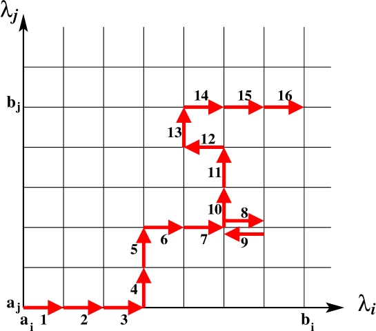
   Figure 3: A schematic representation of the homotopic method shown in pseudo-code form in Fig. 2, for the case of two continuation parameters, $\lambda_{i}$ and $\lambda_{j}$. The figure shows a typical path in the parameter space of $\lambda_{i}$ and $\lambda_{j}$. The arrows show the stepping-directions through parameter space, while the numbers show the order of the stepping sequence. In the first 3 steps we increase the parameter $\lambda_{i}$ with stepping size $\lambda_{i,n_{i+1}}-\lambda_{i,n_{i}}$ (see Fig. 2 for the meaning of $\lambda_{i,n_{i}}$, and note that the stepping size is in general different for different $i$ and/or $n_{i}$). At step 4, a further step in the $\lambda_{i}$ direction produces a problem that does not converge, so we then step forward in the $\lambda_{j}$ direction. After step 5 we find that we can again increase $\lambda_{i}$ until the end of step 8, when we realize that increasing either $\lambda_{i}$ or $\lambda_{j}$ produces divergence. We thus “backtrack” in step 9 and find that we can increase in the $\lambda_{j}$ direction again. We continue with this strategy until we end at step 16, with $\lambda_{i}=b_{i}$ and $\lambda_{j}=b_{j}$.

   Finally, we note that the homotopy method cannot be used without a known initial solution, i.e. a solution to

   $${\mathbf{G}}({\mathbf{x}};a_{1},a_{2},\cdots,a_{p})={\mathbf{0}}\,.$$ (23)

   Although we do not have such a solution, we can tune the parameters $\lambda_{i}$ to the weak field limit $\phi_{(k)}\approx 0$, where Newtonian gravity should be a good approximation to general relativity, and can then use the solution of the Newtonian problem as the initial guess for (23). (Alternately, we can sometimes initialize using a spherically symmetric solution constructed using one of the algorithms described in Chap. A Numerical Study of Boson Stars.)

   As derived in App. A Numerical Study of Boson Stars, the (non-relativistic) Newtonian limit of the coupled Einstein-Klein-Gordon system, yields the following coupled Poisson-Schrödinger system:

   $$i\dot{\phi}(t,{\bf x}) = -\frac{1}{2m}{\rm NewA}^{2}\phi+mV\phi\,,$$ (24)

   $${\rm NewA}^{2}V(t,{\bf x}) = 4\pi m^{2}\phi\phi^{*}\,,$$ (25)

   where $V$ is the Newtonian potential. In the stationary case, and assuming an ansatz

   $$\phi(t,{\mathbf{x}})\longrightarrow e^{-i(E+m)t}\phi({\mathbf{x}})\,,$$ (26)

   the above system reduces to

   $$E{\phi} = -\frac{1}{2m}{\rm NewA}^{2}\phi+mV\phi\,,$$ (27)

   $${\rm NewA}^{2}V = 4\pi m^{2}\phi\phi^{*}\,.$$ (28)

   Numerical experiments reveal that it is easier to solve (27) than System A. In fact, using an algorithm similar to that described above for System A, we can usually find solutions of (27) using suitably chosen gaussian profiles for $\phi$ and $V$. Once the Newtonian solutions (possibly rotating) are in hand, they can be used to start the continuation process for the general relativistic solver.

   As a final remark, we mention that the derivation of the Newtonian limit (see App. A Numerical Study of Boson Stars) was very useful in identifying which approximations had to be satisfied in the weak field limit. In particular, this allowed us to determine whether a particular Newtonian solution was likely to be a good initial guess for the full Einstein-Klein-Gordon system.

4. Underrelaxation:

   Finally, for any value of the continuation parameters, our solution of the 5 coupled elliptic initial value equations proceeds via iteration, such that at each cycle (the Repeat loop of Fig. 2) each of the 5 unknown grid functions is updated in turn. In the notation of Fig. 2 we have $\phi^{l-1}\to\phi^{l}$, $\psi^{l-1}\to\psi^{l}$, etc. in passing from the $l-1$-st iteration to the $l$-th. Empirically, and following Yoshida & Eriguchi [28], we have found it generally useful—and in some cases essential—to adopt an underrelaxation strategy, whereby each grid function, $u^{l}$ is updated using

   $$u^{l}=\omega_{\mathrm{UR}}{\hat{u}}^{l}+\left(1-\omega_{\mathrm{UR}}\right)u^{l-1}\,,$$ (29)

   where $\omega_{\mathrm{UR}}$ is the adjustable underrelaxation parameter and ${\hat{u}}^{l}$ is the “bare” solution computed during the course of the $l$-th pass through the main loop of “IVP_solver”. In many cases we find that we need $\omega_{\mathrm{UR}}<1$ for convergence (hence the terminology “underrelaxation”), although in some situations $\omega_{\mathrm{UR}}>1$ can accelerate convergence (as in the usual case of the successive overrelaxation technique for the solution of discretized elliptic equations). In general, to achieve optimal convergence, $\omega_{\mathrm{UR}}$ must be adjusted on a problem-by-problem basis.

0.20.4 Results

We now present some results computed using the method described in the previous section for the specific cases $k=1$ and $k=2$.

Fig. 4 shows a typical result for the stationary solution of a boson star with angular momentum parameter $k=1$. This solution was computed on a finite difference grid with $N_{\zeta}=129$ and $N_{\theta}=15$, and the convergence criterion for the iteration described in Fig. 2 was ${\rm\epsilon}=10^{-8}$. We remind the reader that for $k=1,2,\cdots$, the complex field vanishes at the origin, and we thus cannot use the central field value to parameterize the continuous family of solutions that exists for each value of $k$. Rather, we parameterize the solutions by choosing (arbitrarily) some point $r=r_{0}$ in the equatorial plane (or, equivalently, $\zeta=\zeta_{0}$), and then specifying the value of the modulus of the scalar field there. Specifically, for the solution shown in Fig. 4 we chose the point $\zeta=0.5$, $s=0$, and set $\phi_{(1)}\equiv\phi_{0}(0.5,0)=0.03$. The plot at the top of Fig. 4 shows the configuration of the scalar field, $\phi_{0}(\zeta,s)$, while the plots below show the various metric components $\alpha,\beta,\psi$ and $\sigma$. In all of the plots, the axis labeled $\zeta$ corresponds to the equatorial plane, $s=0$, or $\theta=\pi/2$, while the far edge of each plot, parallel to the $\zeta$-axis, is $s=1$ and is the azimuthal symmetry axis. (As mentioned in the introductory section of this chapter, we are restricting attention to equatorially-symmetric solutions, and thus only need to solve our equations on a single hemisphere.) The figure shows that the matter distribution for the rotating boson star has—in contrast to spherically symmetric boson stars or rotating fluid stars—toroidal level surfaces (the toroidal nature of a related configuration is clearer in the top plot of Fig. 6 which uses the usual cylindrical coordinates $(\rho,z)$). We also note that the scalar field in this case has a maximum at $\zeta=0.85$, or $r=\zeta/(1-\zeta)=5.7$. We will see that for $k=2$, the maximum value of the scalar field is attained at a larger value of $\zeta$, which implies greater difficulty in constructing solutions at fixed resolution, relative to $k=1$. See Sec. 0.20.5 for further details.

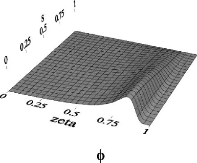
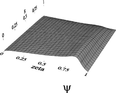
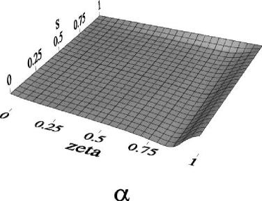
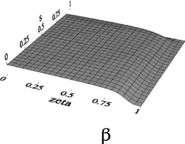
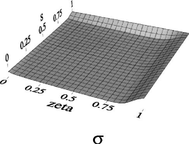
Figure 4: Typical stationary rotating boson star solution with angular momentum parameter, $k=1$. The top plot shows the configuration of the scalar field, which has toroidal level surfaces. The bottom plots show various metric functions. Note that the solutions are symmetric under reflection through the equatorial plane, $s=0$. See the text for additional details concerning the numerical solutions shown here. In lieu of $z$-axes and labels on the above plots (as well as on the other “surface” plots that appear in subsequent figures), we quote the $z$-extrema for the various data sets visualised here: $0.0\leq\phi_{0}(\zeta,s)\leq 0.17$, $1.0\leq\psi(\zeta,s)\leq 1.1$, $0.81\leq\alpha(\zeta,s)\leq 1.0$, $0.0\leq\beta(\zeta,s)\leq 0.014$, $-0.028\leq\sigma(\zeta,s)\leq 0.0$.

Fig. 5 shows a typical stationary boson solution computed for the case $k=2$. In this case the scalar field and its first radial derivative vanish as $r\to 0$, and the stellar configuration is more compact, in the sense that the support of the modulus of the scalar field on the equatorial plane, $\left\{\zeta:|\phi_{0}(\zeta,0)|>\epsilon\right\}$ for some small number $\epsilon$, is of a smaller interval, with a maximum value located further from $r=0$ (but still along the equator) than for $k=1$. Thus the scalar field at $(\zeta,s)=(0.5,0)$ (the point at which we fix $\phi$ for the $k=1$ calculations) will be small and, in fact, may be comparable to the level of numerical error. In other words, the relative error in $\phi_{(2)}$, if fixed at $(0.5,0)$, would be large compared to the $k=1$ case. Clearly, it is more sensible to choose the reference point for $\phi_{(2)}$ closer to the point where the maximum of a typical solution in the $k=2$ family is attained. In this case, we have fixed the solution by specifying $\phi_{(2)}\equiv\phi_{0}(0.875,0)=0.16$. (We note that the maximum value, $\max_{\zeta,s}|\phi_{0}(\zeta,s)|$, of the configuration shown in Fig. 4 is attained at $\zeta=0.89$, or $r=\zeta/(1-\zeta)=8.1$.)

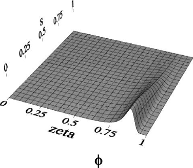
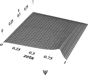
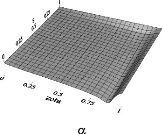
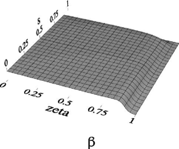
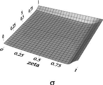
Figure 5: Typical stationary rotating boson star solution with angular momentum parameter, $k=2$. The solutions are symmetric about the equatorial plane. Again, the top plot shows the configuration of the scalar field, which has toroidal level surfaces, while the bottom plots show various metric functions. As with the $k=1$ case, the solutions are symmetric under reflection through the equatorial plane, $s=0$. $0.0\leq\phi_{0}(\zeta,s)\leq 0.18$, $1.0\leq\psi(\zeta,s)\leq 1.2$, $0.75\leq\alpha(\zeta,s)\leq 1.0$, $0.0\leq\beta(\zeta,s)\leq 0.014$, $-0.033\leq\sigma(\zeta,s)\leq 0.0$.

From the top plot in the figure, we see that the boson field again takes on a toroidal shape, with a more completely evacuated “hole” relative to the $k=1$ case. As before, the figures at the bottom show the metric functions, which appear qualitatively the same as the $k=1$ case except that their extrema are located further away from the axis, as we might expect.

It is also instructive to view the scalar field configurations in ordinary cylindrical coordinates, $(\rho,z)$. Fig. 6 shows the two scalar field configurations previously displayed, but now plotted in $(\rho,z)$ coordinates. Since the vertical scales of the two plots are very nearly the same, we can see from the figure that the scalar field has roughly the same maximum amplitude ($\phi_{\mathrm{max}}\approx 0.17$) in the two calculations. It is also clear from the plots that the configuration which ostensibly has the larger angular momentum (i.e. the $k=2$ calculation, bottom plot) has a larger extent than the $k=1$ configuration.

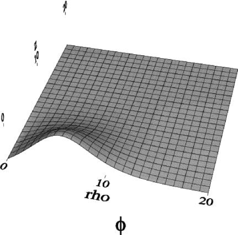
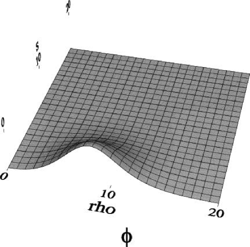
Figure 6: Comparison of scalar field configurations for $k=1$ and $k=2$. These plots show the scalar field solutions previously displayed in Fig. 4 and Fig. 5, but now plotted in cylindrical coordinates $(\rho,z)$. The top and bottom plots show the $k=1$ and $k=2$ results, respectively. We note that the maximum amplitudes of the two scalar fields are comparable for the two cases ($\phi_{\mathrm{max}}\approx 0.17$). $0.0\leq\phi_{0}(\rho,z)\leq 0.17$ for $k=1$, $0.0\leq\phi_{0}(\rho,z)\leq 0.18$ for $k=2$.

As for the case of spherical symmetric boson stars, we can study some of the properties of our rotating configurations as a function of the family parameter (the quantity $\phi_{(k)}$ in this case). In particular, we can produce plots of total mass vs $\phi_{(k)}$ that are completely analogous to Fig. 2. To compute the total mass we use Tolman’s expression [88] (modulo our different convention for the metric signature):

$$M_{\rm Tolman} = \int\left(-2T^{0}{}_{0}+T^{\alpha}{}_{\alpha}\right)\sqrt{|g|}\,d^{3}x$$

$$= \int\frac{\psi^{6}r^{2}\sin\theta e^{\sigma}}{\alpha}\,\phi^{2}\left[2\omega\left(\omega-\beta k\right)-m^{2}\alpha^{2}\right]dr\,d\theta\,d\varphi$$

$$= 4\pi\int^{\infty}_{0}dr\int^{\frac{\pi}{2}}_{0}d\theta\,\frac{\psi^{6}r^{2}\sin\theta e^{\sigma}}{\alpha}\,\phi^{2}\left[2\omega\left(\omega-\beta k\right)-m^{2}\alpha^{2}\right]$$

$$= 4\pi\int^{1}_{0}d\zeta\int^{0}_{1}ds\,\frac{dr}{d\zeta}\,\frac{d\theta}{ds}\frac{\psi^{6}e^{\sigma}}{\alpha}\,\left(\frac{\zeta}{1-\zeta}\right)^{2}\sqrt{1-s^{2}}\,\phi^{2}\left[2\omega\left(\omega-\beta k\right)-m^{2}\alpha^{2}\right]$$

$$= 4\pi\int^{1}_{0}d\zeta\int^{1}_{0}ds\,\frac{\psi^{6}e^{\sigma}}{\alpha}\,\frac{\zeta^{2}}{(1-\zeta)^{4}}\phi^{2}\left[2\omega\left(\omega-\beta k\right)-m^{2}\alpha^{2}\right]\,.$$

Note that for any stationary, asymptotically flat spacetime foliated with spacelike hypersurfaces that are asymptotically orthogonal to the timelike Killing field, the Tolman mass expression is equivalent to the ADM mass [89, 90]. Also note that [26] shows that we have $J=kN$ where $J$ is the total angular momentum defined by

$$J=\int T^{0}{}_{3}\sqrt{-g}\,d^{3}x\,,$$ (30)

and $N$ is the total particle number. Since $N$ has the same qualitative behaviour as a function of ${\phi_{(k)}}$ as $M_{\rm Tolman}$ (and, in fact the calculations of Yoshida & Eriguchi [28]—see Fig. 3 of that reference—show that the numerical values of $N$ and $M_{\rm Tolman}$ are quite similar), with maxima of both quantities achieved at the same value of $\phi_{(k)}$, we can at least qualitatively compare the angular momenta of stars with varying $k$ using the $M_{\rm Tolman}$ vs $\phi_{(k)}$ curve and the relation $J=kN$.

Fig. 7 shows plots of the total mass $M_{\rm Tolman}$ vs the family parameter $\phi_{(k)}$ for rotating boson stars with $k=1$ (top) and $k=2$ (bottom). Again, for $k=1$ we fix the scalar field value, $\phi_{(k)}=\phi_{(1)}$ at $(\zeta,s)=(0.5,0)$, while for $k=2$, where the maximum of $\phi$ tends to be further from the axis, we fix $\phi_{(k)}=\phi_{(2)}$ at $(\zeta,s)=(0.875,0)$. From the plots we can see that in each case, and as for the spherically symmetric calculations, there exists a maximum mass limit above which no stationary solutions exist. We also note that this mass limit appears to increase with the angular momentum parameter, $k$, which is in accord with naive expectations that centrifugal effects due to rotation should partially offset gravitational attraction.

Figure 7: The Tolman mass $M_{\rm Tolman}$ of axisymmetric rotating boson stars with $k=1$ and $k=2$ as a function of family parameter $\phi_{(k)}$. For $k=1$ (top) we fix the scalar field value, $\phi_{(k)}=\phi_{(1)}$ at $(\zeta,s)=(0.5,0)$, while for $k=2$ (bottom), where the maximum of $\phi$ tends to be further from the axis, we fix $\phi_{(k)}=\phi_{(2)}$ at $(\zeta,s)=(0.875,0)$. As in the spherically symmetric case, there exists a maximum mass limit above which no stationary solutions exist.

0.20.5 Some Remarks

Before ending this section we would like to make a few additional remarks:

• While Yoshida & Eriguchi’s code [28] broke down before the maximum-mass star for $k=2$ could be computed, we encounter no difficulties in computing the maximum-mass solution (and beyond) in this case (see Fig. 7). Moreover, we feel that the use of multigrid makes our solution strategy potentially more efficient than previous implementations. In particular, since the multigrid method is capable of solving elliptic PDEs in $O(N)$ time (where $N$ is the number of grid points), in principle there should be no problems in performing high resolution calculations, convergence tests etc. Unfortunately, due to other difficulties we encounter (see below), we are currently unable to perform meaningful convergence tests at this time.

• As discussed in Sec. 0.20.1, the leading order behaviour for $\phi_{0}(r,\theta)$ as $r\to 0$ is $\phi_{0}(r,\theta)=r^{k}\phi_{0k}(\theta)+O(r^{k+2})$. Therefore $\phi_{0}(\zeta,s)|_{\zeta=0}=0$ and $\partial^{i}\phi_{0}(\zeta,s)/\partial\zeta^{i}|_{\zeta=0}=0$ for $i=1,\cdots k-1$. In the multigrid routine we only impose the first condition. Similarly for $\sigma(r,\theta)$ the leading order behaviour as $r\to 0$ is $\sigma(r,\theta)=r^{2}\sigma_{2}(\theta)+O(r^{4})$. In other words $\sigma(\zeta,s)|_{\zeta=0}=0$ and $\partial\sigma(\zeta,s)/\partial\zeta|_{\zeta=0}=0$. Again we only impose the first condition in the multigrid iteration. Moreover, a closer examination of the $r\to 0$ limit of System A, performed via Taylor series expansion of the variables about $r=0$ (for example, we write $\psi(r,\theta)=\psi(0,\theta)+r^{2}\partial^{2}\psi(0,\theta)/\partial r^{2}+O(r^{4})$ and similarly for other variables, and then substitute the expressions into the governing equations (9)-(13)) shows that there are some remaining irregular terms (proportional to $1/r$) that do not explicitly cancel as $r\to 0$. Thus it is perhaps not surprising that our solutions show irregularity near $r=0$ (or equivalently near $\zeta=0$). The fact that we do have some problems with regularity can be seen through close examination of the solutions, which reveals non-smoothness near the $r=0$ “axis” (see Figs. 8 and 9). In particular, Fig. 9 plots the function $\partial\sigma(\zeta,s)/\partial\zeta$ close to the origin $\zeta=0$ for various constant-$s$ slices, $s=0,0.29,0.64$ and 0.93. The function $\sigma(\zeta,s)$ was computed in a calculation with $\phi_{(1)}\equiv\phi_{0}(0.5,0)=0.03$, and using a mesh with $N_{\zeta}=129$ and $N_{s}=15$. Ideally we expect $\partial\sigma(\zeta,s)/\partial\zeta\to 0$ as $\zeta\to 0$. However, the “spikes” in the region $0\leq\zeta\leq 0.05$ clearly show that the regularity condition is not satisfied.

  

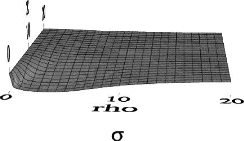
  Figure 8: Regularity problem close to the symmetry axis for $k=1$. This figure shows $\sigma$ for the same solution shown in Figs. 4 and 6, and plotted in cylindrical coordinates $(\rho,z)$. The figure shows that the function is not completely smooth for small $\rho$ (i.e. close to the symmetry axis on the left). $-0.028\leq\sigma(\zeta,s)\leq 0.0$.

  

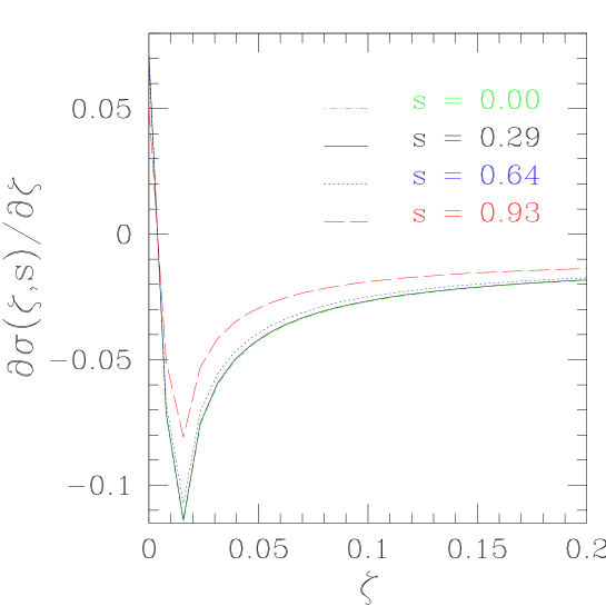
  Figure 9: Irregularity of the metric component $\sigma(\zeta,s)$ as $\zeta\to 0$ for $k=1$. Ideally, these curves should pass linearly through $(0,s)$ as $\Delta\zeta\to 0$. The solution displayed here was computed with $\phi_{(1)}\equiv\phi_{0}(0.5,0)=0.03$ on a computational domain with $N_{\zeta}=129$ and $N_{s}=15$. The figure shows the derivative of $\sigma(\zeta,s)$ with respect to $\zeta$ for constant $s$ slices $s=0,0.29,0.64,0.93$. The “spikes” in the region $0\leq\zeta\leq 0.05$ clearly show that the function $\sigma(\zeta,s)$ does not satisfy the regularity condition $\partial\sigma(0,s)/\partial\zeta=0$.

• As we have seen in Figs. 4 and 5, the larger the value of $k$, the larger the value of $r$ (or $\zeta$) at which $\phi_{0}(\zeta,s)$ is a maximum, and the more concentrated in $(\zeta,s)$ space the stars become. Notice that this increased concentration for increased $k$ is largely a function of our use of the radially compactified coordinate $\zeta$. As $k$ increases, so do the overall diameters of the toroidal regions, and as $r$ increases the corresponding resolution $\Delta r(\zeta)$ decreases. Therefore, as $k$ increases, higher resolution is needed to sufficiently resolve the stationary configurations. A way to remedy this situation is to use a more sophisticated compactification as discussed in Sec. 0.13, as well as in the next section. This will increase the complexity of the system of equations that need to be solved, but will map the location of the scalar field maximum to the central region of the computational domain. In turn, this should partly ameliorate the need for increased resolution for larger values of the angular momentum parameter $k$.

• The maximum Tolman masses $M_{\mathrm{max}}\equiv\max_{\phi_{(k)}}M_{\rm Tolman}(\phi_{(k)})$ we find for rotating boson stars are $M_{\mathrm{max}}=1.72$ for $k=1$ and $M_{\mathrm{max}}=2.44$ for $k=2$. In [27] Yoshida & Eriguchi found that $M_{\mathrm{m}ax}=1.31$ for $k=1$ and $M_{\mathrm{m}ax}\geq 2.40$ for $k=2$. Since their solutions show no irregularity at $r=0$. the discrepancy (which is rather large) may be due to the regularity problems described above.

• As we have discussed several times, following [27] we parametrize each family of solutions for $k=1,2,\cdots$ by specifying the value of ${\phi_{(k)}}$ at some arbitrary point $(\zeta,s)=(\zeta_{0},0)$. Within the context of our current particular finite difference solution of System A, this approach has the advantage that it is very easy to implement. However, from a theoretical point of view it seems more natural to instead specify the $k$-th radial derivative of the scalar field. This could be implemented by defining a new scalar function $\bar{\phi}_{0}(\zeta,s)$ such that [91]

  $$\phi_{0}(\zeta,s)=\zeta^{k}\bar{\phi_{0}}(\zeta,s)\,,$$ (31)

  and rewriting System A for $\bar{\phi_{0}}(\zeta,s)$. In this new system we would then specify $\partial^{(k)}_{\zeta}\phi_{0}(\zeta,s)|_{\zeta=0}$ as the family parameter, eliminating the ad hoc parameter $\zeta_{0}$ from the algorithm. We discuss the initial steps of the implementation of such an approach in the next section.

• We can replace the individual updates of each variable in the main iteration of our initial data solver (the Repeat loop in Fig. 2) by combining the independent multigrid updates shown in Figure 2 into a single multigrid solve for the five fields. More specifically, in the new solver, a basic relaxation step would visit a given grid location $(\zeta_{i},s_{j})$ and simultaneously update the 5 grid function values $\phi_{i,j},\psi_{i,j}\cdots\sigma_{i,j}$ using a 5-dimensional Newton method. Thus, each pointwise update in this case would require us to set up and solve a $5\times 5$ linear system, rather than 5 scalar linear equations. The $5\times 5$ solve is more costly computationally, as well as being more tedious to set up since the full Jacobian must be computed. A key advantage is that the underrelaxation (UR) part of the algorithm is no longer needed for convergence.

• As in the study of dynamics of boson stars in spherical symmetry, we could study the dynamics of boson stars with angular momentum in axisymmetry, using the solutions constructed in this section as initial data for the dynamical code. However, as mentioned in the introductory section of this chapter, the coordinate conditions adopted in graxi (see (46)) are not compatible with our ansatz (7). More precisely, if we assume the metric has the form (46) and the boson star has the form (7), then the real and imaginary parts of the Klein-Gordon equation (45) will yield different equations for $\phi_{0}(r,\theta)$. The incompatibility can be traced to the coordinate choice made in adopting the form (46) whereby the metric component $g_{t\varphi}(\rho,z)$ is required to vanish [52]. To easily study the dynamics of the rotating boson stars constructed here, we would need to adopt a different form for the metric ($g_{t\varphi}(\rho,z)\neq 0$), which in turn would require substantial modifications to graxi. We have not yet pursued this possibility.

0.20.6 A Proposal for an Improved Rotating Boson Star Solver (System B)

In the previous section we discussed the difficulties we encountered in constructing equilibrium solutions of rotating boson stars: we have regularity problems near $\zeta=0$, the maximal values of the scalar field are achieved at larger $\zeta$ on the equatorial plane for increasing $k$, and the configurations are increasingly concentrated in the $\zeta$-$s$ plane for increasing $k$. In this section we suggest a way of rewriting System A to treat these problems. A new code based on this approach is under development, but at this point we do not have any results to report.

Following [28, 92] we write the metric in the form

$$ds^{2}=-e^{\eta+\delta}dt^{2}+e^{2\psi}\left(d\rho^{2}+dz^{2}\right)+e^{\eta-\delta}\rho^{2}\left(d\varphi-\beta dt\right)^{2}\,,$$ (32)

where $\eta,\delta,\psi$ and $\beta$ are functions of the cylindrical coordinates $\rho$ and $z$ only. (We note that [28, 92] use spherical-polar coordinates.) The motivation for the above specific form is that a detailed analysis (again, by Taylor series expansion of the variables about $\rho=0$ with subsequent substitution of the expansions in the equations given below) shows that all equations described below are manifestly regular as $\rho\to 0$, provided that the $\rho=0$ conditions demanded by local flatness on-axis are imposed. Also motivated by regularity considerations, we define a new scalar field variable $\bar{\phi_{0}}(\rho,z)$ by

$$\phi_{0}(\rho,z)=\rho^{k}\bar{\phi_{0}}(\rho,z)\,,$$ (33)

so that we explicitly factor out the leading order $\rho\to 0$ behaviour of the field. The Klein-Gordon equation, Hamiltonian constraint, momentum constraint and the equations for $\eta$ and $\delta$ are derived in a manner similar to that used in defining the corresponding equations for System A. For notational simplicity, we drop the “0” subscript and the bar so that $\bar{\phi_{0}}(\rho,z)\to\phi(\rho,z)$. We also choose $\kappa=1$ instead of $8\pi$ as previously, and continue to set $m=1$. We then have System B:

$$\begin{split}\phi_{,\rho\rho}+\phi_{,zz}+\left(\eta_{,\rho}+\frac{1+2k}{\rho}\right)\phi_{,\rho}+\eta_{,z}\phi_{,z}+\left(e^{2\psi-\eta-\delta}(\omega+\beta k)^{2}-e^{2\psi}+\frac{\eta_{,\rho}k}{\rho}+\frac{1-e^{2\psi-\eta+\delta}}{\rho^{2}}k^{2}\right)\phi\,,\end{split}$$ (34)

$$\begin{split}\psi_{,\rho\rho}+\psi_{,zz}-\frac{1}{4}e^{-2\delta}\rho^{2}\left(\beta_{,\rho}^{2}+\beta_{,z}^{2}\right)+\frac{1}{4}\left(\delta_{,\rho}^{2}+\delta_{,z}^{2}-\eta_{,\rho}^{2}-\eta_{,z}^{2}\right)-\frac{1}{2\rho}\left(\eta_{,\rho}+\delta_{,\rho}\right)\\ +\frac{\rho^{2k}}{2}\left(\phi_{,\rho}^{2}+\phi_{,z}^{2}\right)+\rho^{2k-1}k\phi\phi_{,\rho}+\frac{\phi^{2}\rho^{2k}}{2}\left[\left(\omega+\beta k\right)^{2}e^{2\psi-\delta-\eta}+\frac{k^{2}}{\rho^{2}}\left(1-e^{2\psi+\delta-\eta}\right)\right]=0\,,\end{split}$$ (35)

$$\beta_{,\rho\rho}+\beta_{,zz}+\left(-2\delta_{,\rho}+\eta_{,\rho}+\frac{3}{\rho}\right)\beta_{,\rho}+\left(\eta_{,z}-2\delta_{,z}\right)\beta_{,z}-2e^{2\psi-\eta+\delta}\rho^{2k-2}\phi^{2}k(w+\beta k)=0\,,$$ (36)

$$\eta_{,\rho\rho}+\eta_{,zz}+{\eta_{,\rho}}^{2}+\frac{2\eta_{,\rho}}{\rho}+{\eta_{,z}}^{2}+\phi^{2}\rho^{2k}\left[e^{2\psi}-e^{2\psi-\eta-\delta}\left(\omega+\beta k\right)^{2}+\frac{k^{2}e^{2\psi-\eta+\delta}}{\rho^{2}}\right]=0\,,$$ (37)

$$\begin{split}\delta_{,\rho\rho}+\delta_{,zz}+\left(\eta_{,\rho}+\frac{1}{\rho}\right)\delta_{,\rho}+\eta_{,z}\delta_{,z}+\phi^{2}\rho^{2k}\left[-e^{2\psi-\eta-\delta}\left(\omega+\beta k\right)^{2}-\frac{k^{2}e^{2\psi-\eta+\delta}}{\rho^{2}}\right]\\ -e^{-2\delta}\left({\beta_{,\rho}}^{2}+{\beta_{,z}}^{2}\right)\rho^{2}-\frac{\eta_{,\rho}}{\rho}=0\,.\end{split}$$ (38)

Further, we compactify both coordinates via coordinate transformations $\rho\to\zeta(\rho)$ and $z\to\mu(z)$ given by

$$\zeta = \frac{\rho}{\rho_{0}+\rho}\,,$$ (39)

$$\mu = \frac{z}{z_{0}+z}\,.$$ (40)

The new parameters $\rho_{0}$ and $z_{0}$ can be chosen to map arbitrary coordinate lines $\rho=\rho_{0}$ and $z=z_{0}$ to $\zeta=1/2$ and $\mu=1/2$, respectively, in the new coordinates (see Sec. 0.13). Fig. 10 illustrates the effect of such a transformation. Rewriting System B in $(\zeta,\mu)$ coordinates is straightforward but leads to lengthy expressions that will not be given here.

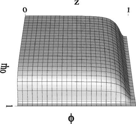
Figure 10: Demonstration of the effect of adjusting the coordinate-transformation parameters $\rho_{0}$ and $z_{0}$. The top figure shows a typical initial configuration of $\bar{\phi_{0}}(\zeta,\mu)$ with $\rho_{0}=1$ and $z_{0}=1$. The lower figure shows the same configuration, but now with $\rho_{0}=10$ and $z_{0}=10$. $0.0\leq\phi_{0}(\rho,z)\leq 0.01$.

To ensure System B is regular at $\rho=0$ (or equivalently, $\zeta=0$) we apply the locally-flat condition $2\psi(0,\mu)-\eta(0,\mu)+\delta(0,\mu)=0$. The other regularity conditions are

$$\phi_{,\zeta}(0,\mu)=\psi_{,\zeta}(0,\mu)=\beta_{,\zeta}(0,\mu)=\eta_{,\zeta}(0,\mu)=\delta_{,\zeta}(0,\mu)=0\,,$$ (41)

and the other boundary conditions are:

$$\phi(1,\mu)=\psi(1,\mu)=\beta(1,\mu)=\eta(1,\mu)=\delta(1,\mu)=0\,,$$ (42)

$$\phi(\zeta,1)=\psi(\zeta,1)=\beta(\zeta,1)=\eta(\zeta,1)=\delta(\zeta,1)=0\,,$$ (43)

$$\phi_{,\mu}(\zeta,0)=\psi_{,\mu}(\zeta,0)=\beta_{,\mu}(\zeta,0)=\eta_{,\mu}(\zeta,0)=\delta_{,\mu}(\zeta,0)=0\,.$$ (44)

We can now parametrize the family by the value of $\phi(\zeta,\mu)\equiv\bar{\phi_{0}}(\zeta,\mu)$ at $\zeta=0$ and $\mu=0$. The multigrid solver will use point-wise simultaneous relaxation of all five unknowns defined at each grid point (using a 5-dimensional Newton method) as described in Sec. 0.20.5.

0.21 Dynamics of Axisymmetric Non-rotating Boson Stars

In this section we focus on the dynamics of axisymmetric non-rotating boson stars. In the first subsection we present the equations of motion that are to be solved, and that have been derived using the (2+1)+1 formalism outlined in Chap. A Numerical Study of Boson Stars. We note that this derivation is not original to this work, nor is the basic code (graxi) that implements the discrete version of the equations [9, 8]. However, as mentioned previously, we have extended graxi so that it can be initialized with data for the complex scalar field representing one or more spherical boson stars in an overall axisymmetric configuration.

In subsequent subsections we perform two classes of numerical experiments. The first class involves the head-on collision of equal-mass boson stars, where each star can be boosted towards the other via an adjustable initial linear momentum parameter, $p_{z}$. The second class involves perturbation of stable boson stars with a massless real scalar field, generalizing the calculations in spherically symmetry that were described in Chap. A Numerical Study of Boson Stars. In both instances, we study the critical behaviour that arises at the threshold of black hole formation. We find evidence for Type I transitions in both cases, as well as evidence for scaling of the lifetime, $\tau(p)$, of near-critical configurations

$$\tau(p)\sim-\gamma\ln|p-p^{\star}|\,,$$ (45)

that one normally associates with Type I behaviour ($p$ is, as usual, the family parameter that is tuned to generate the critical solution). As far as we are aware, this represents the first instance of the observation of Type I critical phenomena in an axisymmetric, general relativistic model. In addition, we show evidence for interesting “solitonic” behaviour of interacting boosted boson stars, similar to that previously seen in Newtonian computations [32].

0.21.1 The equations of motion

We choose cylindrical coordinates $(t,\rho,z,\varphi)$, impose spatial coordinate conditions so that the 2-dimensional spatial metric (i.e. the metric in the $(\rho,z)$ plane) is conformally flat, and adopt 3-maximal slicing (i.e. the trace of the 3-dimensional curvature tensor $K_{ij}$ vanishes). As mentioned above, we also restrict attention to the non-rotating case. The spacetime metric then has the form [9]

$$ds^{2}=\left\{-\alpha^{2}+\psi^{4}\left[(\beta^{\rho})^{2}+(\beta^{z})^{2}\right]\right\}dt^{2}+2\psi^{4}\left(\beta^{\rho}d\rho+\beta^{z}dz\right)dt+\psi^{4}\left(d\rho^{2}+dz^{2}+\rho^{2}e^{2\rho\bar{\sigma}}d\varphi^{2}\right)\,,$$ (46)

where $\alpha$, $\beta^{\rho}$, $\beta^{z}$, $\psi$, and $\bar{\sigma}$ are functions of $\rho,z$ and $t$ only. The reason for using $\bar{\sigma}$ (in contrast to the seemingly more natural variable $\sigma\equiv\rho\bar{\sigma}$) as a fundamental metric function is motivated by regularity considerations. In particular the leading order behaviour of $\bar{\sigma}$ in the limit as $\rho\to 0$ is $\bar{\sigma}(\rho,z)=\rho\sigma_{1}(z)+O(\rho^{3})$, which can be implemented numerically as a Dirichlet boundary condition. On the other hand the leading order behaviour of $\sigma$ is $\sigma(\rho,z)=\rho^{2}\sigma_{2}(z)+O(\rho^{4})$, and is much more difficult to maintain via finite-differencing of the type used in this thesis.

From (46) we see that the squared-norm, $s^{2}$, of the rotational Killing vector (see (24)) is given by

$$s^{2}=\psi^{4}\rho^{2}e^{2\rho\bar{\sigma}}\,.$$ (47)

Without angular momentum, the twist vector $\omega^{\alpha}$ (see 25) vanishes.

We write the evolution equation for $\bar{\sigma}$ in first-order-in-time form by introducing an auxiliary variable $\bar{\Omega}$ defined by

$$\rho\bar{\Omega} \equiv -2\,{}^{(2)}K^{\rho}\,_{\rho}-\,{}^{(2)}K^{z}\,_{z}$$ (48)

$$= \frac{2}{s}n^{a}\partial_{a}s+\frac{\beta^{z}\,_{,z}-\beta^{\rho}\,_{,\rho}}{2\alpha}\,,$$ (49)

where $n^{a}$ is the future-directed, unit-norm, timelike vector orthogonal to the $t={\rm const.}$ hypersurfaces of the dimensionally reduced 2+1 spacetime, and ${}^{(2)}K^{\rho}\,_{\rho},{}^{(2)}K^{z}\,_{z}$ are the components of the extrinsic curvature on those hypersurfaces. Again, the choice of this particular form for $\bar{\Omega}$ was motivated by regularity concerns; certain terms that behave as $1/\rho$ as $\rho\to 0$, and which would otherwise appear in the equations of motion for the variable naturally conjugate to $\bar{\sigma}$, manifestly cancel with the definition (48). We also note that the leading order behaviour of $\bar{\Omega}$ in the limit as $\rho\to 0$ is $\bar{\Omega}(\rho,z)=\rho\bar{\Omega}_{1}(z)+O(\rho^{3})$.

We now adopt a slightly modified form for the stress-energy tensor of the complex scalar field

$$T_{\mu\nu}\equiv T^{\phi}_{\mu\nu}\equiv\left[\left({\rm NewA}_{\mu}\phi{\rm NewA}_{\nu}\phi^{\ast}+{\rm NewA}_{\nu}\phi{\rm NewA}_{\mu}\phi^{\ast}\right)-g_{\mu\nu}\left(\ {\rm NewA}^{\alpha}\phi{\rm NewA}_{\alpha}\phi^{\ast}+m^{2}|\phi|^{2}+2\lambda|\phi|^{4}\right)\right]\,.$$ (50)

(Note that the definition differs from that in (44) by an overall factor of 2). In particular, we have added a quartic self-interaction term, $2\lambda|\phi|^{4}$ to the scalar field Lagrangian, where $\lambda$ is an adjustable coupling constant that will satisfy $\lambda=0$ for some of the simulations shown below and $\lambda=1$ in other instances. We note that in addition to the parameter (the particle mass) $m$ which sets the length scale of the system, the addition of the self-interaction term introduces a new dimensionless parameter, $\lambda$, into the model, and that our results will generally now depend on the specific value of $\lambda$ that is used. In what follows, we have used non-vanishing self-interaction primarily as a vehicle to allow us to probe the black hole threshold in certain cases. Additional details will be provided in Sec. 0.21.2.

We also define the auxiliary complex scalar variable $\Pi$ via

$$\Pi\equiv n^{a}\partial_{a}\phi\,,$$ (51)

so that the Klein-Gordon equation for $\phi$ can be recast as a set of first-order-in-time equations.

In Sec. 0.21.5 we use a real scalar field to perturb the boson stars, analogously to what was done in Sec. 0.17.2 in the spherical case. Therefore we again introduce a real massless scalar field $\phi_{3}(t,\rho,z)$ with a stress energy tensor

$$T_{\mu\nu}^{\phi_{3}}\equiv 2{\rm NewA}_{\mu}\phi_{3}{\rm NewA}^{\mu}\phi_{3}-g_{\mu\nu}{\rm NewA}^{\alpha}\phi_{3}{\rm NewA}_{\alpha}\phi_{3}\,.$$ (52)

The equation of motion for this field is

$${\rm NewA}^{\mu}{\rm NewA}_{\mu}\phi_{3}=0\,,$$ (53)

and, once more, we define an auxiliary field $\Pi_{3}$

$$\Pi_{3}\equiv n^{a}\partial_{a}\phi_{3}\,,$$ (54)

so that (53) can be cast in first-order form.

We note that $\phi,\Pi,\phi_{3}$ and $\Pi_{3}$ are functions of $\rho,z$ and $t$ only. Since the scalar field $\phi=\phi_{1}+i\phi_{2}$ and its conjugate momentum $\Pi=\Pi_{1}+i\Pi_{2}$ are complex, we now have 12 fundamental real variables $\alpha,\beta^{\rho},\beta^{z},\psi,\bar{\sigma},\bar{\Omega},\phi_{1},\phi_{2},\phi_{3},\Pi_{1},\Pi_{2}$ and $\Pi_{3}$ that must be evolved.

As mentioned above (and as for the case of the study of dynamical spherically symmetric boson stars in Chap. A Numerical Study of Boson Stars), we choose to implement maximal slicing, so that the trace of the 3-dimensional extrinsic curvature tensor of $t={\mbox{\rm const.}}$ slices within the 4-dimensional manifold (not to be confused with the trace of the 2-dimensional extrinsic curvature tensor ${}^{(2)}K$ in the 2+1 dimensionally reduced spacetime) is zero

$${}^{(3)}K=0\,.$$ (55)

This condition provides the following elliptic equation for $\alpha$

$$2\left(\rho\alpha_{,\rho}\right)_{,\rho^{2}}+\alpha_{,zz}+\alpha_{,\rho}\left(2\frac{\psi_{,\rho}}{\psi}+\left(\rho\bar{\sigma}\right)_{,\rho}\right)+\alpha_{,z}\left(2\frac{\psi_{,z}}{\psi}+\left(\rho\bar{\sigma}\right)_{,z}\right)$$

$$-\frac{\psi^{4}}{2\alpha}\left[(\beta^{\rho}{}_{,\rho}-\beta^{z}{}_{,z})^{2}+(\beta^{\rho}{}_{,z}+\beta^{z}{}_{,\rho})^{2}\right]-\frac{\psi^{4}}{6\alpha}\left[2\alpha\rho\bar{\Omega}+\beta^{\rho}{}_{,\rho}-\beta^{z}{}_{,z}\right]^{2}$$

$$+8\pi\psi^{4}\alpha\left(m^{2}|\phi|^{2}+\lambda|\phi|^{4}-2|\Pi|^{2}\right)-16\pi\alpha\Pi_{3}^{2}=0\,.$$ (56)

The ADM decomposition in the dimensionally reduced 2+1 spacetime will result in one Hamiltonian constraint and two momentum constraints, which, when combined with the demand that the $(\rho,z)$ 2-spaces be conformally flat, provides elliptic equations for $\psi$, and for $\beta^{\rho}$ and $\beta^{z}$, respectively. They are

$$8\frac{\psi_{,\rho\rho}}{\psi}+8\frac{\psi_{,zz}}{\psi}+16\frac{\psi_{,\rho^{2}}}{\psi}+8\left(\rho\bar{\sigma}\right)_{,\rho}\frac{\psi_{,\rho}}{\psi}+8\left(\rho\bar{\sigma}\right)_{,z}\frac{\psi_{,z}}{\psi}$$

$$+{\psi^{4}\over 2\alpha^{2}}\left[(\beta^{\rho}{}_{,\rho}-\beta^{z}{}_{,z})^{2}+(\beta^{z}{}_{,\rho}+\beta^{\rho}{}_{,z})^{2}\right]+{\psi^{4}\over 6\alpha^{2}}\left[2\alpha\rho\bar{\Omega}+\beta^{\rho}{}_{,\rho}-\beta^{z}{}_{,z}\right]^{2}$$

$$=-16\pi\left(\psi^{4}\left(m^{2}|\phi|^{2}+\lambda|\phi|^{4}+|\Pi|^{2}\right)+|\phi_{,z}|^{2}+|\phi_{,\rho}|^{2}\right)-6\left(\rho^{2}\left(\rho\bar{\sigma}\right)_{,\rho}\right)_{,\rho^{3}}$$

$$-2\left(\left(\rho\bar{\sigma}\right)_{,\rho}\right)^{2}-2\left(\rho\bar{\sigma}\right)_{,zz}-2\left(\left(\rho\bar{\sigma}\right)_{,z}\right)^{2}-16\pi\left(\Pi_{3}^{2}+\phi_{3,\rho}^{2}+\phi_{3,z}^{2}\right)\,,$$ (57)

$$\begin{split}\frac{2}{3}\beta^{\rho}{}_{,\rho\rho}+\beta^{\rho}{}_{,zz}+\frac{1}{3}\beta^{z}{}_{,z\rho}+32\pi{\alpha\over\psi^{2}}\Pi_{3,\rho}+16\pi\alpha\left(\phi_{,\rho}\Pi^{\ast}+\phi_{,\rho}^{\ast}\Pi\right)\\ -\left(\left(\frac{\alpha_{,z}}{\alpha}-6\frac{\psi_{,z}}{\psi}\right)-\left(\rho\bar{\sigma}\right)_{,z}\right)\left(\beta^{z}{}_{,\rho}+\beta^{\rho}{}_{,z}\right)\\ -\frac{2}{3}\left(\frac{\alpha_{,\rho}}{\alpha}-6\frac{\psi_{,\rho}}{\psi}\right)\left[\beta^{\rho}{}_{,\rho}-\beta^{z}{}_{,z}\right]-\frac{8}{3}\alpha\bar{\Omega}-\frac{2\alpha\rho}{3}\left[6\bar{\Omega}\frac{\psi_{,\rho}}{\psi}+\bar{\Omega}_{,\rho}+3\bar{\Omega}\left(\rho\bar{\sigma}\right)_{,\rho}\right]=0,\end{split}$$ (58)

and

$$\beta^{z}{}_{,\rho\rho}+\frac{4}{3}\beta^{z}{}_{,zz}-\frac{1}{3}\beta^{\rho}{}_{,z\rho}+\left[\left(\rho\bar{\sigma}\right)_{,\rho}+\frac{2\alpha}{\psi^{6}}\left(\frac{\rho\psi^{6}}{\alpha}\right)_{,\rho^{2}}\right]\left(\beta^{\rho}{}_{,z}+\beta^{z}{}_{,\rho}\right)$$

$$+\left[2\left(\rho\bar{\sigma}\right)_{,z}-\frac{4}{3}\left(\frac{\alpha_{,z}}{\alpha}-6\frac{\psi_{,z}}{\psi}\right)\right]\left(\beta^{z}{}_{,z}-\beta^{\rho}{}_{,\rho}\right)-\frac{2\alpha\rho}{3}\left(6\bar{\Omega}\frac{\psi_{,z}}{\psi}+\bar{\Omega}_{,z}\right)$$

$$+32\pi{\alpha\over\psi^{2}}\Pi_{3,z}+16\pi\alpha\left(\phi_{,z}\Pi^{\ast}+\phi_{,z}^{\ast}\Pi\right)-2\alpha(\bar{\sigma}_{,z})\rho^{2}\bar{\Omega}=0\,.$$ (59)

The evolution equation for $\bar{\sigma}$ is, with the definition of $\bar{\Omega}$ (48), given by

$$\dot{\bar{\sigma}}=2\beta^{\rho}\left(\rho\bar{\sigma}\right)_{,\rho^{2}}+\beta^{z}\bar{\sigma}_{,z}-\alpha\bar{\Omega}-\left[{\beta^{\rho}\over\rho}\right]_{,\rho}\,,$$ (60)

where, as usual, an over-dot denotes a time derivative. The evolution equation for $\bar{\Omega}$ is

$$\dot{\bar{\Omega}}=2\beta^{\rho}\left(\rho\bar{\Omega}\right)_{,\rho^{2}}+\beta^{z}\bar{\Omega}_{,z}-{1\over 2\alpha\rho}\left(\beta^{z}{}_{,\rho}{}^{2}-\beta^{\rho}{}_{,z}{}^{2}\right)+{1\over\psi^{4}}\left({\alpha_{,\rho}\over\rho}\right)_{,\rho}$$

$$+{\alpha\over\psi^{6}}\left({(\psi^{2})_{,\rho}\over\rho}\right)_{,\rho}-{2\alpha\over\psi^{4}}\left(4\frac{\psi_{,\rho^{2}}}{\psi}+\left(\rho\bar{\sigma}\right)_{,\rho^{2}}\right)\left(\frac{\alpha_{,\rho}}{\alpha}+\frac{2\psi_{,\rho}}{\psi}\right)$$

$$-{\alpha\over\psi^{4}}\left[\bar{\sigma}_{,z}\left(\frac{\alpha_{,z}}{\alpha}+\frac{2\psi_{,z}}{\psi}\right)+\rho\bar{\sigma}_{,z}{}^{2}+\bar{\sigma}_{,zz}\right]+64\pi{\alpha\over\psi^{4}}\rho(\phi_{3,\rho^{2}})^{2}+16\pi\frac{\alpha}{\rho\psi^{4}}|\phi_{,\rho}|^{2}\,.$$ (61)

The definition of $\Pi$ and the Klein-Gordon equation give

$$\dot{\phi}=\beta^{\rho}\phi_{,\rho}+\beta^{z}\phi_{,z}+{\alpha}\Pi\,,$$ (62)

and

$$\dot{\Pi}=\beta^{\rho}\Pi_{,\rho}+\beta^{z}\Pi_{,z}-\alpha\phi\left(2\lambda|\phi|^{2}+m^{2}\right)+\frac{2\alpha}{\psi^{5}}\left(\psi_{,\rho}\phi_{,\rho}+\psi_{,z}\phi_{,z}\right)$$

$$+\frac{1}{\psi^{4}}\left[\alpha\left(\left(\rho\bar{\sigma}\right)_{,\rho}\phi_{,\rho}+\left(\rho\bar{\sigma}\right)_{,z}\phi_{,z}\right)+\phi_{,\rho\rho}+\phi_{,zz}+\frac{\phi_{,\rho}}{\rho}+\alpha_{,\rho}\phi_{,\rho}+\alpha_{,z}\phi_{,z}\right]\,.$$ (63)

The definition of $\Pi_{3}$ (54) and the wave equation for $\phi_{3}$ (53) gives

$$\dot{\phi_{3}}=\beta^{\rho}\phi_{3,\rho}+\beta^{z}\phi_{3,z}+{\alpha\over\psi^{2}}\Pi_{3},$$ (64)

and

$$\dot{\Pi_{3}}=\beta^{\rho}\Pi_{3,\rho}+\beta^{z}\Pi_{3,z}+{1\over 3}\Pi_{3}\left(\alpha\rho\bar{\Omega}+2\beta^{\rho}_{,\rho}+\beta^{z}_{,z}\right)$$

$$+\frac{1}{\psi^{4}}\left[2\left(\rho\alpha\psi^{2}\phi_{3,\rho}\right)_{,\rho^{2}}+\left(\alpha\psi^{2}\phi_{3,z}\right)_{,z}\right]+\frac{\alpha}{\psi^{2}}\left[\left(\rho\bar{\sigma}\right)_{,\rho}\phi_{3,\rho}+\left(\rho\bar{\sigma}\right)_{,z}\phi_{3,z}\right]\,.$$ (65)

The regularity conditions on the symmetry axis are

$$\alpha_{,\rho}(t,0,z)=\psi_{,\rho}(t,0,z)=\beta^{z}_{,\rho}(t,0,z)=\beta^{\rho}(t,0,z)=\bar{\sigma}(t,0,z)=\bar{\Omega}(t,0,z)=0\,,$$ (66)

$$\phi_{1,\rho}(t,0,z)=\phi_{2,\rho}(t,0,z)=\phi_{3,\rho}(t,0,z)=\Pi_{1,\rho}(t,0,z)=\Pi_{2,\rho}(t,0,z)=\Pi_{3,\rho}(t,0,z)=0\,.$$ (67)

The outer boundary conditions we use, applied at $\rho=\rho_{\rm max}$, $z=z_{\rm max}$ and $z=z_{\rm min}$, are

$$\alpha-1+\rho\alpha_{,\rho}+z\alpha_{,z} = 0,$$

$$\psi-1+\rho\psi_{,\rho}+z\psi_{,z} = 0,$$

$$\beta^{z}+\rho\beta^{z}_{,\rho}+z\beta^{z}_{,z} = 0,$$

$$\beta^{\rho}+\rho\beta^{\rho}_{,\rho}+z\beta^{\rho}_{,z} = 0,$$

$$r\bar{\sigma}_{,t}+\rho\bar{\sigma}_{,\rho}+z\bar{\sigma}_{,z}+\bar{\sigma} = 0,$$

$$r\bar{\Omega}_{,t}+\rho\bar{\Omega}_{,\rho}+z\bar{\Omega}_{,z}+\bar{\Omega} = 0,$$

$$r\phi_{1,t}+\rho\phi_{1,\rho}+z\phi_{1,z}+\phi_{1} = 0,$$

$$r\phi_{2,t}+\rho\phi_{2,\rho}+z\phi_{2,z}+\phi_{2} = 0,$$

$$r\phi_{3,t}+\rho\phi_{3,\rho}+z\phi_{3,z}+\phi_{3} = 0,$$

$$r\Pi_{1,t}+\rho\Pi_{1,\rho}+z\Pi_{1,z}+\Pi_{1} = 0,$$

$$r\Pi_{2,t}+\rho\Pi_{2,\rho}+z\Pi_{2,z}+\Pi_{2} = 0,$$

$$r\Pi_{3,t}+\rho\Pi_{3,\rho}+z\Pi_{3,z}+\Pi_{3} = 0,$$ (68)

where $r\equiv\sqrt{\rho^{2}+z^{2}}$.

Thus, the system of equations (0.21.1)-(68) consists of 4 elliptic PDEs (the equations for $\alpha,\psi,\beta^{\rho}$ and $\beta^{z}$), and 8 first-order-in time evolution equations (also PDEs) that are hyperbolic in nature. The finite differencing of the above equations is given in [8], with trivial modifications for the extra terms involving the components $\phi_{1},\phi_{2}$ of the complex scalar fields, and their conjugates $\Pi_{1},\Pi_{2}$. $\phi_{3}$ is identified with the original scalar field described in [9]. The finite difference scheme also incorporates Kreiss-Oliger style dissipation, with a dissipation coefficient, $\epsilon_{d}$, similar to that defined in (40). Again the interested reader can find full details in [8].

Following modification to accommodate boson star initial data, the graxi code was subjected to convergence tests to ensure that the discrete equations of motion had been implemented correctly. Results from one such test are described in App. A Numerical Study of Boson Stars.

Since we study dynamics of non-rotating boson stars in this section, we can use static spherically symmetric boson star solutions generated using one of the codes described in Chap. A Numerical Study of Boson Stars, as the basis for setting up axisymmetric initial data. However, even for the seemingly trivial case where we evolve a single spherical star using graxi, the initial data setup is slightly complicated by the fact that we need to transform the spherically symmetric solution $\phi_{0}(r)$ to the $(\rho,z)$ coordinates used in graxi. We thus generally need to interpolate radially symmetric data onto the discrete domain $(\rho_{i},z_{j})$, possibly translating the data so that the center of the star lies at some specified location along the $z$-axis. Here we use standard polynomial (Lagrange) interpolation which is fourth order in the mesh spacings $(\Delta\rho,\Delta z)$. Fig. 11 shows a typical result of the interpolation process. Also note that all simulations in this section are done with the adaptive mesh refinement (AMR) capability provided by graxi, in order to effectively resolve the various length and time scales encountered during the dynamical evolution of the scalar fields. In particular, the complex field tends to form configurations that are considerable more compact at late times than at the initial time, especially in cases where black holes form.

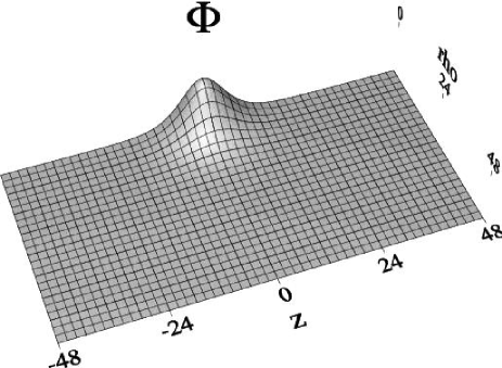
Figure 11: A typical scalar field configuration, $\phi_{0}(\rho,z)$ (denoted as $\Phi$), given by interpolation of a spherically symmetric (1D) boson star solution to a 2D finite difference mesh in cylindrical coordinates, $(\rho,z)$. $0.0\leq\phi_{0}(\rho,z)\leq 0.014$.

0.21.2 Head-on Collisions of Boson Stars—Setup of Numerical Experiments

The PDEs solved in the simulations discussed here are those listed in Sec. 0.21.1. The initial data for the (first) boson star, always chosen from the stable branch, is given by interpolation of a static spherically symmetric star as just described. The interpolated data, $\phi_{0}^{(1)}(\rho,z)$, are then scaled by

$$\phi_{0}^{(1)}(\rho,z)\to\frac{1}{\sqrt{2}}\phi_{0}^{(1)}(\rho,z)\,,$$ (69)

since the definitions (44) and (50) differ by a factor of 2. The star is then “boosted” (roughly speaking, given an initial momentum) via (see [87, 32])

$$\phi^{(1)}(\rho,z;p_{z}^{(1)})\equiv\phi^{(1)}_{0}(\rho,z)\,e^{ip^{(1)}_{z}z}\,,$$ (70)

where $p_{z}^{(1)}$ is the parameter that controls the magnitude of the boost, and which we will refer to as the initial momentum parameter, or, more loosely, as the initial momentum.

The boosted boson star is then translated so that the center of the star is located at some specified point, $(0,z_{1})$, on the axis of symmetry

$$\phi^{(1)}(\rho,z;p_{z}^{(1)},z_{1})\equiv T\left(\phi^{(1)}(\rho,z;p_{z}^{(1)})\,;z_{1}\right)\,,$$ (71)

where $T$ is the translation operator defined by

$$T(f(\rho,z)\,;z_{1})\equiv\left\{\begin{array}[]{ll}f(\rho,z-z_{1})&z-z_{1}\in[z_{\rm min},z_{\rm max}]\\ 0&\rm{otherwise}\end{array}\right.\,,$$ (72)

and $z_{1}$ is another adjustable parameter.

Similarly we construct another boosted boson star centered at $(0,z_{2})$ via

$$\phi^{(2)}(\rho,z;p_{z}^{(2)},z_{2})\equiv T\left(\phi^{(2)}(\rho,z;p_{z}^{(2)})\,;z_{2}\right)\,,$$ (73)

and, finally, the complex scalar field per se is initialized to be the sum of the configurations representing the two boosted, translated stars

$$\phi(0,\rho,z)=\phi^{(1)}(\rho,z;p_{z}^{(1)},z_{1})+\phi^{(2)}(\rho,z;p_{z}^{(2)},z_{2})\,.$$ (74)

In the simulations described below we have always considered identical stars (i.e. $\phi_{0}^{(1)}(\rho,z)\equiv\phi_{0}^{(2)}(\rho,z)\equiv\phi_{0}(\rho,z)$), each of which is boosted towards the other with the same initial “speed”, (i.e. $-p_{z}^{(2)}\equiv p_{z}^{(1)}\equiv p_{z}$). We note that the solutions generated from such initial data are symmetric with respect to the equatorial plane, but that we do not make explicit use of this fact in the calculations. We also note that there is nothing in principle that prevents us from carrying out simulations with $\phi_{0}^{(1)}(\rho,z)\neq\phi_{0}^{(2)}(\rho,z)$ and/or $-p_{z}^{(2)}\neq p_{z}^{(1)}$.

In addition to the complex field, $\phi$, we must also supply initial values for the conjugate variable $\Pi$. To this end we define a contribution, $\Pi^{(1)}(\rho,z;p_{z}^{(1)})$, associated with the first star

$$\Pi^{(1)}(\rho,z;p_{z}^{(1)})=\omega_{1}\phi^{(1)}(\rho,z;p_{z}^{(1)})-\beta^{\rho}(\rho,z)\partial_{\rho}\phi^{(1)}(\rho,z;p_{z}^{(1)})-\beta^{z}(\rho,z)\partial_{z}\phi^{(1)}(\rho,z;p_{z}^{(1)})\,,$$ (75)

where $\omega_{1}$ is the eigenvalue of the first boson star. We similarly define a contribution, $\Pi^{(2)}(\rho,z;p_{z}^{(2)})$, for the second star

$$\Pi^{(2)}(\rho,z;p_{z}^{(2)})=\omega_{2}\phi^{(2)}(\rho,z;p_{z}^{(2)})-\beta^{\rho}(\rho,z)\partial_{\rho}\phi^{(2)}(\rho,z;p_{z}^{(2)})-\beta^{z}(\rho,z)\partial_{z}\phi^{(2)}(\rho,z;p_{z}^{(2)})\,,$$ (76)

and then initialize $\Pi$ via

$$\Pi(0,\rho,z)=T\left(\Pi^{(1)}(\rho,z;p_{z}^{(1)})\,;z_{1}\right)+T\left(\Pi^{(2)}(\rho,z;p_{z}^{(2)})\,;z_{2}\right)\,.$$ (77)

The remaining freely specifiable variables $\sigma(t,\rho,z)$ and $\bar{\Omega}(t,\rho,z)$, (which can be associated with the gravitational wave content of the spacetime), are initialized to zero:

$$\sigma(0,\rho,z)=\bar{\Omega}(0,\rho,z)=0\,.$$ (78)

Finally, initial values for the remaining geometric variables, $\alpha,\beta^{\rho},\beta^{z}$ and $\psi$, are determined from the constraint and slicing equations.

In the simulations we typically use a Courant factor $\Delta t/\Delta\rho=\Delta t/\Delta z=0.2$ or $0.3$, and the dissipation coefficient is $\epsilon_{d}=0.5$.

0.21.3 Head-on Collisions—Solitonic Behaviour

In the head-on collisions of Newtonian boson stars (i.e. in simulations involving the solution of a coupled Poisson-Schrödinger system—see App. A Numerical Study of Boson Stars) it has been observed that the stars sometimes exhibit “solitonic” behaviour [32]. This behaviour is a function of the Newtonian analog of the initial momentum parameter, $p_{z}$, defined above. Specifically, for small initial momenta the stars simply merge together to form a single star, while for sufficiently large initial momenta, the stars pass through each other as if there was no interaction between them. We have carried out numerical experiments similar to those described in [32], but using the fully coupled general-relativistic equations of motion. We find that solitonic behaviour also occurs in this case for large values of the initial momentum.

In Fig. 12 we show results from a typical simulation of a head-on collision of two boosted boson stars with no self-interaction ($\lambda=0$). The boson stars are initially centered at $(0,z_{1})=(0,-25)$ and $(0,z_{2})=(0,25)$ and have initial momenta $-p_{z}^{(2)}=p_{z}^{(1)}=0.4$. The computational domain is $0\leq\rho\leq 50$, $-50\leq z\leq 50$. From the figure we see that the stars seem to pass through each other as if there were little net interaction between them.

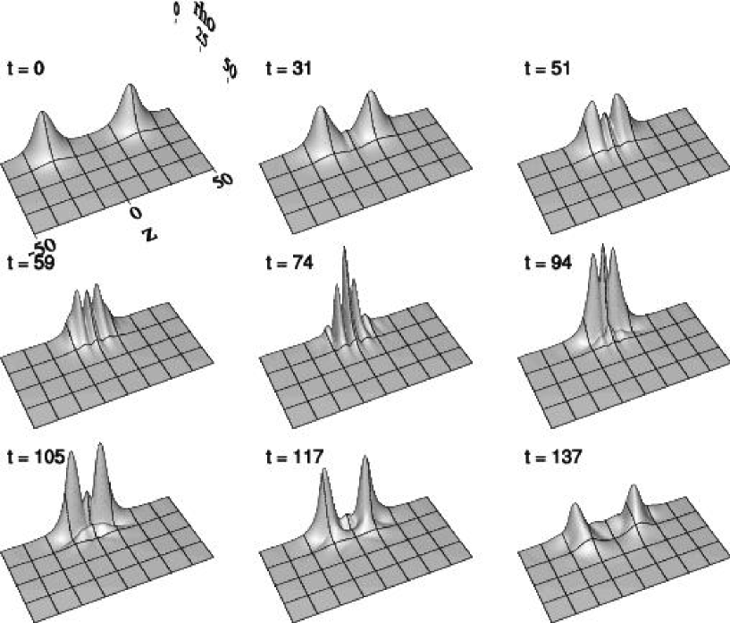
Figure 12: Typical solitonic behaviour in a head-on collision of boson stars. The stars are initialized via interpolation, translation and boosting of a spherically symmetric solution with $\phi_{0}(0)=0.02$. The stars are initially centered at $(0,-25)$ and $(0,25)$, with initial momenta $-p_{z}^{(2)}=p_{z}^{(1)}=p_{z}=0.4$. The two stars start to overlap at $t\approx 31$, interfere with each other, and then separate at $t\approx 117$. Other simulation parameters are: $\Delta t/\Delta z=\Delta t/\Delta\rho=0.2$, $\Delta\rho=\Delta z=0.78$. Note that the temporal spacing between successive snapshots is not constant—the time instants displayed have been chosen to illustrate the key features of the simulation. $0.0\leq|\phi(t,\rho,z)|\leq 0.03$.

0.21.4 Head-on Collisions—Critical Behaviour

We now proceed to study critical behaviour in the context of head-on collisions of boson stars with equatorial-plane symmetry. For sufficiently large values of $\phi_{0}(0)$ (for instance, $\phi_{0}(0)=0.02$), variation of the initial momentum parameter, $p_{z}$, generates a family of solutions that interpolates through the black hole threshold; however, in this case the sense of $p_{z}$ is reversed from the normal situation—i.e. for small (large) $p_{z}$ black holes do (do not) form. Once we have determined an initial bracket for $p_{z}$ that is known to span the threshold, we can, in principle, tune the parameter to the critical value $p^{\star}_{z}$ that generates a critical solution.

However, in our early tuning experiments—which involved no self-interaction for the complex field—we found it difficult to determine whether or not a black hole would form in the evolution as $p_{z}$ approached the critical value. The addition of the quartic self-interaction term provides the stars with more binding, and reduces the distortion in their shapes during the collision. This allows us to identify whether a particular calculation is subcritical or supercritical, and we are then generally able to determine a value of $p^{\star}_{z}$ to machine precision. We note that we only incorporate the interaction term into the dynamical equations; i.e. we do not compute static boson stars that include the quartic term.  Thus, with self-interaction turned on, the initial data prescription described above will no longer generate a static solution for a single boson star, and in fact, we find that in the evolution of data computed with $\lambda\neq 0$ the central amplitude of the complex field tends to grow in time. However, within the time scale for black hole formation in near-critical evolutions ($t\approx 300$), and for the value $\lambda=1$ that we have adopted for the simulations described in this section, this growth in amplitude appears to be insignificant.

Also, we need to remark at this point that when we speak of the black hole threshold in the head-on collision calculations described here, we are referring to what we might call “prompt” black hole formation, i.e. whether a black hole forms during the initial merger phase of the collision. Calculations which are subcritical with respect to this definition are generated by relatively large values of $p_{z}$, and are characterized by the re-appearance of two star-like configurations following the initial merger phase (see Fig. 18). Subsequently, however, the stars will re-merge and then typically form a black hole (again, see Fig. 18). However, this fact that subcritical simulations may eventually form black holes does not interfere with our ability to study the threshold defined with respect to prompt collapse.

We now discuss the results from the study of a specific family of head-on collisions in which Type I critical phenomena are observed. As in the calculation discussed in the previous sub-section, initial data for any member of the family of solutions describe two identical stars ($\phi_{0}(0)=0.02$) centered at $(0,-25)$ and $(0,25)$, and with initial momenta $-p_{z}^{(2)}=p_{z}^{(1)}=p_{z}$. The stars are thus well separated from each other at $t=0$. The computational domain is $-50\leq z\leq 50$, $0\leq\rho\leq 50$, and the base resolution is $(N_{\rho},N_{z})=(129,257)$, yielding base mesh spacings $\Delta\rho=\Delta z=0.390625$. As many as 6 additional levels of 2:1 refinement are employed in the calculations, so that the finest available resolution is $\Delta\rho=\Delta z=0.006104$. The critical parameter value for this family of data is $p^{\star}_{z}\approx 0.21$.

Fig. 13 shows snapshots of $|\phi(t,\rho,z)|$ from a simulation with $p_{z}=0$, so that the stars are initially at rest. The time development clearly shows that the two boson stars attract each other through their mutual gravitational interaction. At $t\approx 400$ the stars begin to merge, and subsequently they form a configuration which approximates that of a single star. Following the merger, the configuration oscillates—emitting some energy in the form of outgoing scalar radiation in the process—then collapses and forms a black hole.

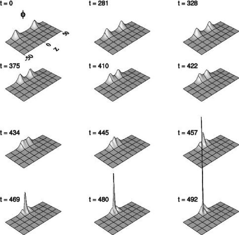
Figure 13: Head-on collision of boson stars with $p_{z}=0$. Plotted here is the modulus of the complex field, $|\phi(t,\rho,z)|$. The identical stars ($\phi_{0}=0.02$) are initially centered at $(0,-25)$ and $(0,25)$. They move towards one another due to their mutual gravitational attraction, then start to merge at $t\approx 400$. The resulting configuration oscillates and radiates energy during the merger phase, and then collapses to form a black hole—an apparent horizon is first detected at $t=492$ (see Fig. 16). See the text for additional details of the numerical parameters of the simulation. $0.0\leq|\phi(t,\rho,z)|\leq 0.19$.

Fig. 14 shows the variation of the maximum value of the modulus of the scalar field, $|\phi|_{\rm max}(t)\equiv\mathrm{max}_{\rho,z}|\phi(t,\rho,z)|$, vs $t$, again for the case $p_{z}=0$. This function initially has a value of $0.014$ (note that since (44) and (50) differ by a factor of 2, the value here is not 0.02). As the evolution proceeds it exhibits oscillations (presumably due to gravitationally induced perturbations of each of the stars and/or the quartic self-interaction). until $t\approx 430$, when the stars begin to merge. At this time, $|\phi|_{\rm max}(t)$ begins to rapidly increase, and this behaviour signals the imminent formation of a black hole (see Fig. 16). Fig. 15 shows the variation of the ADM mass, $M_{\mathrm{ADM}}$ vs $t$, for the same calculation ($M_{\rm ADM}$ is computed using (2.67) of [8]). The figure indicates that a small amount of mass is radiated from the system during the simulation.

Figure 14: Maximum value of scalar field modulus $|\phi|_{\rm max}(t)\equiv\max_{\rho,z}|\phi(t,\rho,z)|$ vs time for a head-on boson star collision with $p_{z}=0$. $|\phi|_{\rm max}(t)$ oscillates during the in-fall phase (presumably due to gravitationally induced distortions of the stars and/or the quartic self-interaction), then starts to grow rapidly during the merger phase, $t>430$, signalling the collapse of the configuration (analogous to central density increasing in fluid collapse) and the imminent formation of a black hole.

Figure 15: ADM mass vs time for a head-on boson star collision with $p_{z}=0$. Although there are slight oscillations in this quantity at early times (most likely related to outer boundary effects), the mass shows an overall decrease in time, indicating that energy is being radiated from the system.

Finally, Fig. 16 shows the time development of the apparent horizon detected in the simulation at late times—an apparent horizon is first found at $t=492$. We note that this figure simply shows the location of the apparent horizon in coordinate space for various times and that much of the “dynamics” that is visible is probably attributable to coordinate effects. In particular, the proper surface areas of the apparent horizons (which we expect ultimately to be closely tied to the black hole mass) are not directly correlated to the coordinate areas covered by each of the contours. Computation of the former requires evaluation of an integral involving $\psi(t,\rho,z)^{4}$, and $\psi$ is a highly dynamical quantity, that tends to rapidly increase in the central regions of the domain at late times. Thus, although we have not explicitly computed the area of the apparent horizon, we anticipate that it is non-decreasing.

Figure 16: Development of the apparent horizon for a head-on collision of boson stars with $p_{z}=0$. Five snapshots of the coordinate location of the apparent horizon are shown for $t=491.8,494.0,496.9,498.8$ and $503.2$ (an apparent horizon is first detected at $t=492$). As discussed in the text, much of the “dynamics” of the horizon that is visible here is likely attributable to coordinate effects. In particular, contrary to what the figure suggests, we expect the area of the apparent horizon to be a monotonically increasing quantity.

Fig. 17 shows the time development of $|\phi(t,\rho,z)|$ for a marginally supercritical head-on collision. Here, the momentum parameter, $p_{z}\approx 0.21$ has been tuned to criticality to within a relative precision $\Delta p_{z}/p_{z}=O(10^{-15})$. In this calculation, (and due to the non-zero initial boost) the stars merge at a significantly earlier time—$t\approx 90$—than for $p_{z}=0$ (compare with Fig. 14). Following the merger, we estimate that the configuration enters the critical state at $t\approx 140$, and remains in that state (with some oscillations) until a black hole forms. An apparent horizon is detected at $t=280$, and we note that the final black hole will contain most of the mass-energy of the configuration at that time. That is, the smallest-mass black hole that can be formed via variation of $p_{z}$ has finite mass, as is characteristic of a Type I transition.

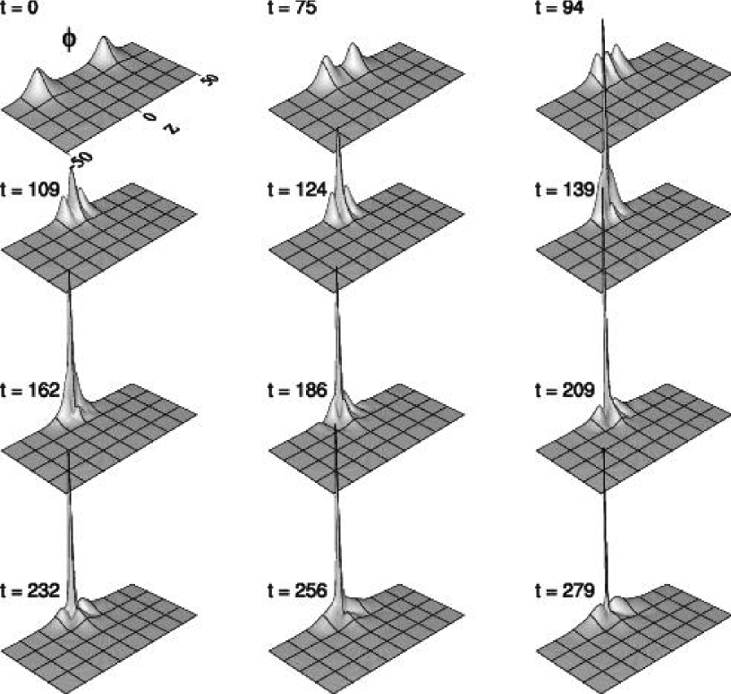
Figure 17: Marginally supercritical, head-on boson star collision. The time development of $|\phi(t,\rho,z)|$ is plotted for a supercritical calculation with $p_{z}$ tuned to roughly machine precision of the critical value $p^{\star}_{z}\approx 0.21$. The stars merge at $t\approx 90$, significantly earlier than in the simulation shown in Fig. 14. The resulting merged configuration remains in the critical state for $\Delta t\approx 130$, then collapses to form a black hole. An apparent horizon is first detected at $t=280$. $0.0\leq|\phi(t,\rho,z)|\leq 0.13$.

Similarly, Fig. 18 shows the time development of $|\phi(t,\rho,z)|$ for a marginally subcritical head-on collision. Again, the momentum parameter, $p_{z}\approx 0.21$ has been tuned to criticality to within a relative precision $\Delta p_{z}/p_{z}=O(10^{-15})$. At early times the evolution here is indistinguishable from that of the supercritical data. However, in contrast to the supercritical case, at $t\approx 280$ two star-like configurations begin to reappear and are clearly distinguishable as separate stars at $t\approx 390$. Since the initial momenta of the stars is moderate, the overall system is gravitationally bound and the two stars re-merge and form a black hole. An apparent horizon is detected at $t=570$.

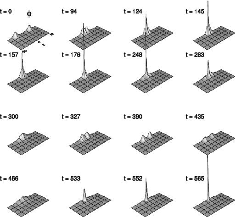
Figure 18: Marginally subcritical, head-on boson star collision. The time development of $|\phi(t,\rho,z)|$ is plotted for a subcritical calculation with $p_{z}$ tuned to roughly machine precision of the critical value $p^{\star}_{z}\approx 0.21$. At early times the evolution here is indistinguishable from that shown in Fig. 17. However, in contrast to the supercritical case, at $t\approx 280$ two star-like configurations begin to reappear and are clearly distinguishable as separate stars at $t\approx 390$. Since the initial momenta of the stars is moderate, the overall system is gravitationally bound and the two stars re-merge and form a black hole. An apparent horizon is detected at $t=570$. $0.0\leq|\phi(t,\rho,z)|\leq 0.14$.

Finally, Fig. 19 shows the time of black hole formation (time of first appearance of an apparent horizon) $t_{\mathrm{BH}}$ plotted as a function of $\log|p_{z}-p_{z}^{\ast}|$. The plot provides strong evidence for scaling of the lifetime, $\tau$, of the critical configuration of the form

$$\tau=-\gamma\log\left|p_{z}-p_{z}^{\ast}\right|\,,$$ (79)

with a value $\gamma=6.6$ computed from a least squares fit. Again, observation of such scaling is consistent with a Type I transition in the model.

There remains the question as how the critical solution observed in this study can itself be characterized. Although we have not yet studied this matter in detail, we hypothesize that the solution can be described in terms of a static boson star on the unstable branch, superimposed with (largely) normal-mode oscillations that are not necessarily spherically symmetric.

Figure 19: Scaling law for near critical evolutions of head-on boson star collisions The time of black hole formation (time of first appearance of an apparent horizon), $t_{\mathrm{BH}}$, is plotted vs $\log|p_{z}-p_{z}^{\ast}|$. The linearity of the data provides evidence for lifetime scaling associated with a Type I transition, as previously seen in the spherically symmetric calculations described in Chap. A Numerical Study of Boson Stars.

0.21.5 Perturbation of Boson Stars by an Aspherical Real Scalar Field

In this section we present results from a second study of critical phenomena involving boson stars in axisymmetry. In this case the calculations generalize those described in Chap. A Numerical Study of Boson Stars, where a massless scalar field was used to induce collapse of the boson star. In particular, the massless scalar field configuration is not spherically symmetric in the simulations described below.

For this class of experiment, the initial data for the complex field, $\phi$, is simply a single, stable boson star centered at the origin, $(\rho,z)=(0,0)$. As previously, we use a star with $\phi_{0}(0)=0.02$. The initial data for the real scalar field takes the form of a “generalized gaussian”

$$\phi_{3}(0,\rho,z)=A_{3}\exp\left[-\left(\frac{\sqrt{(\rho-\rho_{0})^{2}+\epsilon(z-z_{0})^{2}}-R_{0}}{\Delta}\right)^{2}\right]\,,$$ (80)

where $A_{3}$, $\rho_{0}$, $z_{0}$, $\Delta$, $R_{0}$ and $\epsilon$ are all adjustable parameters. In the calculations described below we set $\rho_{0}=0$, $z_{0}=0$, $\Delta=4$, $\epsilon=0.4$ and $R_{0}=25$. We note that for $\rho_{0}=z_{0}=0$, $\epsilon$ controls the “ellipticity” of the initial pulse, while $R_{0}$ controls how far the pulse is from the origin at $t=0$. The overall amplitude factor, $A_{3}$ is the parameter that is tuned to generate a critical solution, and we find $A^{\star}_{3}\approx 0.013$. We also note that we specify initial data for the conjugate variable $\Pi_{3}$ so that the massless field is almost purely incoming at the initial time.

The computational domain is $-75\leq z\leq 75$, $0\leq\rho\leq 75$, and the base resolution is $(N_{\rho},N_{z})=(193,385)$, yielding base mesh spacings $\Delta\rho=\Delta z=0.390625$. We again allow up to 6 additional levels of 2:1 refinement, so that the finest available resolution is $\Delta\rho=\Delta z=0.006104$.

Fig. 20 shows the time development of $|\phi(t,\rho,z)|$ and $\phi_{3}(t,\rho,z)$ for a marginally supercritical perturbed boson star. For clarity the subplots display only a portion of the computational domain, namely $-50\leq z\leq 50$, $0\leq\rho\leq 50$. The top 6 subplots in the figure depict the evolution of the boson star, which approximates the critical solution for a period of $\Delta t\approx 70$, before forming a black hole. An apparent horizon is first detected at $t\approx 220$. The bottom 6 subplots show the corresponding evolution of the real scalar field, which leaves the computational domain at $t\approx 110$, at which time the boson star is still in a near-critical configuration. Fig. 21 displays corresponding results from a marginally subcritical evolution, in which there are indications that the end state of evolution is a stable boson star with large amplitude oscillations.

Thus, we see that the type of non-spherical perturbation used here leads to the same type of behaviour seen in the spherically-symmetric calculations, at least at the qualitative level. Among other things, this suggests that the unstable static boson stars do not develop additional unstable axisymmetric modes when the restriction to spherical symmetry is relaxed (or, if such modes do exist, that their growth rates are quite small in comparison to that of the unstable spherical mode).

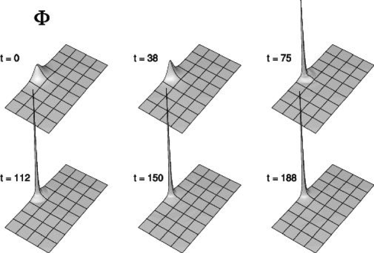
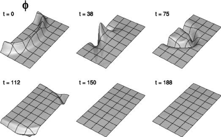
Figure 20: Perturbation of a boson star (denoted $\Phi$) by an elliptical in-going real scalar field (denoted $\phi$). This figure shows the time development of $|\phi(t,\rho,z)|$ and $\phi_{3}(t,\rho,z)$ for a marginally supercritical simulation, with tuning parameter $A_{3}\approx 0.013$ (see (80)). While the simulation domain is $0\leq\rho\leq 75$, $-75\leq z\leq 75$, for clarity only the region $0\leq\rho\leq 50$, $-50\leq z\leq 50$ is shown. After the massless scalar field implodes through the boson star, the boson star enters its critical state, oscillates about it for a while, and then collapses to form a black hole. An apparent horizon is first detected at $t\approx 220$. $0.0\leq|\phi(t,\rho,z)|\leq 0.13$ (denoted as $\Phi$), $-0.056\leq\phi_{3}(t,\rho,z)\leq 0.021$ (denoted as $\phi$).

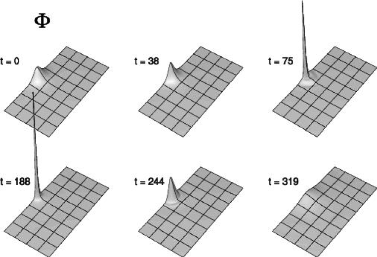
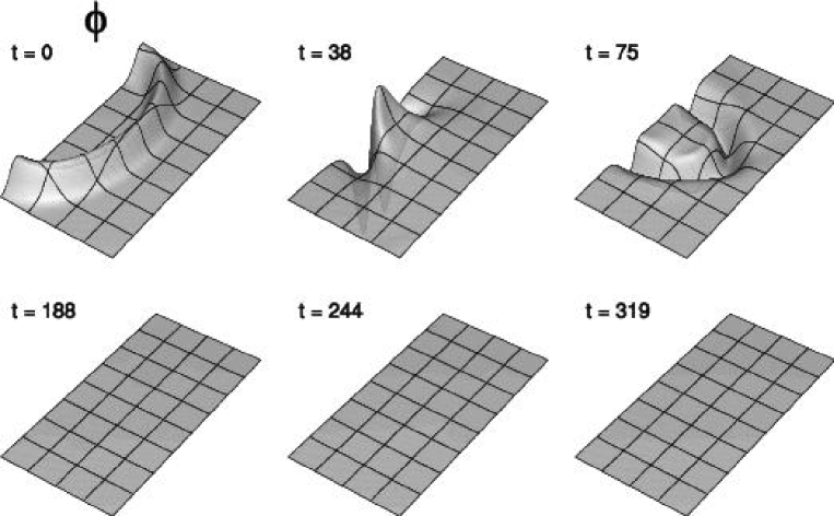
Figure 21: This figure shows the time development of $|\phi(t,\rho,z)|$ and $\phi_{3}(t,\rho,z)$ for a marginally subcritical simulation (i.e. for $A_{3}$ of the order of machine epsilon smaller than the value used for the simulation shown in Fig. 20). In this case there are indications that the late time configuration will be a stable boson star with large amplitude oscillations, as seen in the spherical calculations of Chap. A Numerical Study of Boson Stars. $0.0\leq|\phi(t,\rho,z)|\leq 0.13$ (denoted as $\Phi$), $-0.056\leq\phi_{3}(t,\rho,z)\leq 0.021$ (denoted as $\phi$).

We can again plot the time of black hole formation against $\log|p-p^{\ast}|$ to measure the expected lifetime scaling for near critical evolutions, as shown in Fig. 22. Once more we verify that the expected Type I scaling holds.

Figure 22: Lifetime scaling law for near critical evolutions for boson stars perturbed by non-spherical real scalar field. The time of black hole formation $t_{\mathrm{BH}}$ is plotted as a function of $\log|p-p^{\ast}|$. The expected (Type I) scaling of the lifetime of the critical configuration is again observed.

Before concluding this chapter, we want to make two additional observations concerning the axisymmetric evolutions that we have performed. The first one concerns non-radial oscillations of perturbed boson stars, while the second one concerns the linear momentum of such stars. We note that we have not studied either matter in much detail, deferring such work to the future.

When boson stars are perturbed in a non-spherical manner, we observe that, as expected, the stars exhibit oscillations which are not strictly radial. Not surprisingly, non-radial oscillations are more pronounced when we use a very aspherical distribution of real scalar field as the perturbing agent. In Fig. 24 we show the evolution of such a highly non-radial configuration of real scalar field. We can see from the figure that the initial data consists of several distinct pulses located at different positions in the $\rho$-$z$ plane. Specifically, the initial configuration of the massless field is given by

$$\phi_{3}(0,\rho,z)=A_{3}\exp\left[-\left(\frac{\sqrt{(\rho-\rho_{0}+\rho_{1}-\rho_{2}-\rho_{3})^{2}+\epsilon(z-z_{0})^{2}}-R_{0}}{\Delta}\right)^{2}\right]\cos n\theta\,,$$ (81)

where

$$\rho_{1} = \tilde{A}\exp\left[-\left(\frac{z}{\tilde{\Delta}}\right)^{2}\right]\,,$$ (82)

$$\rho_{2} = \tilde{A}\exp\left[-\left(\frac{z-z_{c}}{\tilde{\Delta}}\right)^{2}\right]\,,$$ (83)

$$\rho_{3} = \tilde{A}\exp\left[-\left(\frac{z+z_{c}}{\tilde{\Delta}}\right)^{2}\right]\,,$$ (84)

and $\tan\theta=\rho/z$. We have chosen $\tilde{A}=5$, $\tilde{\Delta}=8$, $z_{c}=35$, $n=8$, and have set all other parameters to the values used in the previously described set of computations. For clarity, we again display only a portion of the solution domain, namely $-50\leq z\leq 50$ and $0\leq\rho\leq 50$. Fig. 24 displays the corresponding evolution of the boson star, where now the part of the solution domain given by $-20\leq z\leq 20$ and $0\leq\rho\leq 20$ is shown. The figure plots various contour lines of $|\phi(t,\rho,z)|$ as a function of time, and non-radial oscillations of the star are clearly visible.

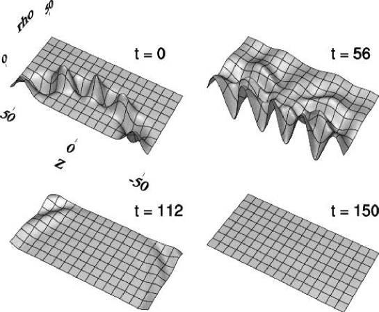
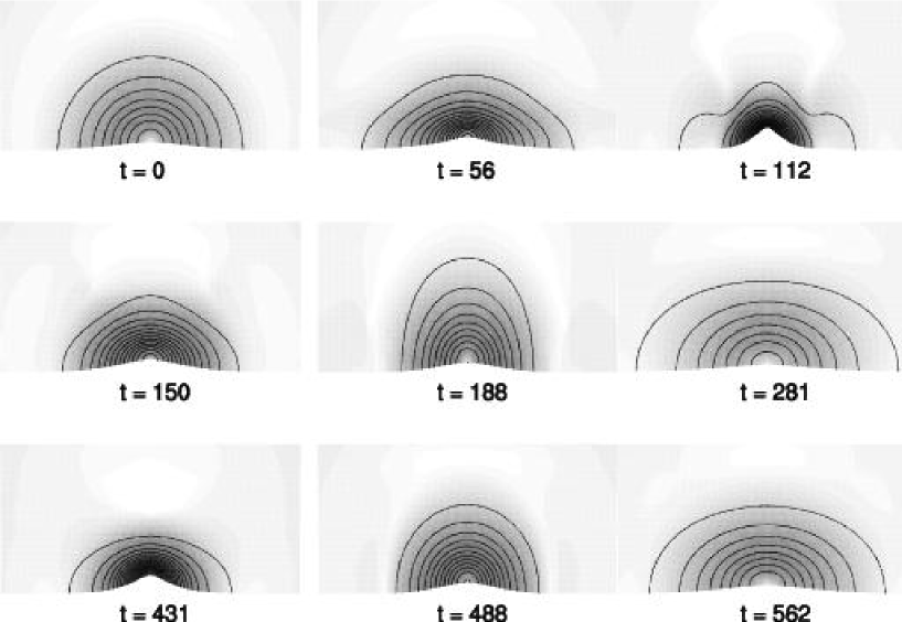
Figure 23: Dynamical evolution of non-radial distribution of perturbing real scalar field. The initial configuration of the real scalar field is given by (81). $-0.023\leq\phi_{3}(t,\rho,z)\leq 0.022$.

Figure 24: Dynamical evolution of boson star as a result of non-radial perturbation by a real scalar field. The snapshots show both radial and non-radial oscillations of the star. $0.0\leq|\phi(t,\rho,z)|\leq 0.049$.

In Figs. 25 and 26 we show another evolution of a boson star perturbed by an in-going non-radial distribution of real scalar field. The boson star is initially located at $(0,-7.8125)$. Again the evolution is solved on a domain $-75\leq z\leq 75$, $0\leq\rho\leq 75$, while the figures show a portion of the domain, $-50\leq z\leq 50$, $0\leq\rho\leq 50$. The initial configuration for the real scalar field is the same as for the previous calculation, except that we choose $n=9$ and restrict the support of the real scalar field to $z\geq 0$. Thus the real scalar field is not symmetric about the equatorial plane in this case. Fig. 25 shows that at early times, although the modulus of the complex field oscillates, the boson star remains at a fixed coordinate location. At $t\approx 80$ most of the real scalar field has passed through the boson star, and the boson star apparently starts to move in the positive $z$ direction, with the amplitude of the complex field still oscillatory. Fig. 26 shows the corresponding evolution of the real scalar field.

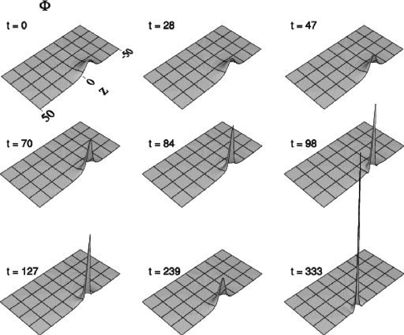
Figure 25: Evolution of a boson star as a result of perturbation by a non-radial perturbing real scalar field, that is not symmetric about the equatorial plane. The boson star appears to remain at the same location $z\approx-8$ until $t\approx 80$, when most of the real scalar field has passed through the star. The star then appears to move in the positive $z$ direction at a speed of 0.09. $0.0\leq|\phi(t,\rho,z)|\leq 0.14$ (denoted as $\Phi$).

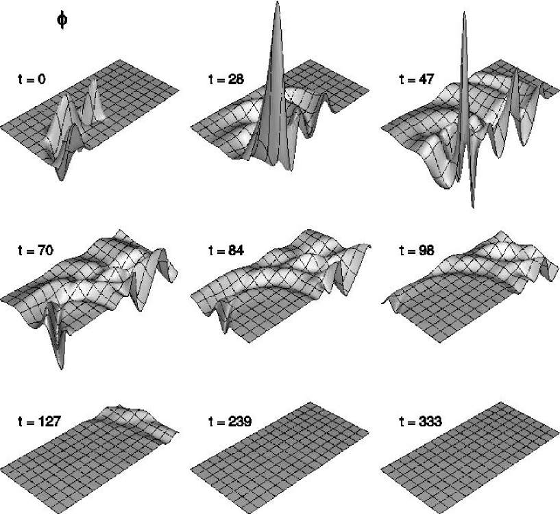
Figure 26: Evolution of non-radial, non-equatorially-symmetric distribution of perturbing real scalar field. Here the real field, whose support at the initial time is confined to $z>0$, passes through the boson star at $t\approx 80$, and leaves the computational domain at $t\approx 130$. $-0.047\leq\phi_{3}(t,\rho,z)\leq 0.090$ (denoted as $\phi$).

Fig. 27 shows the maximum of the modulus of the complex scalar field, $\max_{z}|\phi(t,0,z)|$, on-axis as a function of time $t$, as well as the $z$-coordinate of the maximum $z^{\phi}_{\max}(t)$ defined by

$$\phi(t,0,z^{\phi}_{\rm{max}}(t))=\max_{z}|\phi(t,0,z)|\,.$$ (85)

From the graph we can see that the maximum remains at $z\approx-8$ until $t\approx 80$, at which point it acquires a non-zero velocity which apparently settles down to a speed of about 0.09. However, this apparent motion of the boson star seems to be primarily a coordinate effect. Fig. 28 shows the value of $-\min_{z}\beta^{z}(t,0,z)$ as a function of time $t$, as well as the apparent velocity of the boson star (which exhibits several jumps since the value $\max|\phi(t,0,z)|$ is not smooth). The two functions appear to be of the same order of magnitude, consistent with the conjecture that the motion is mainly due to the particular coordinates that we have chosen.

Figure 27: The maximum value of the boson star modulus on-axis $\max_{z}\left(|\phi(t,0,z)|\right)$ ($\times 10^{2}$) and the $z$ location of that maximum as a function of time. The boson star starts to move at $t\approx 80$, and attains a constant final speed of $0.09$.

Figure 28: Velocity of boson star and the negative of the minimum of the shift component $\beta_{z}(t,0,z)$ as a function of time $t$. The two functions are of the same order of magnitude, indicating that the movement of the boson star depicted in Fig. 27 is primarily due to the particular coordinates we have chosen.

Chapter 0 Conclusions and Future Work

In this thesis we have performed numerical simulations of general relativistic boson stars in both spherically and axially symmetric spacetime. The principal new results are as follows.

In the spherically symmetric case, we studied Type I critical phenomena associated with boson stars. In particular, contrary to some previous claims, we found that the end state of subcritical evolution is a stable boson star executing large amplitude oscillations, that can largely be understood as excitations of the fundamental normal mode of the end-state star. For the particular example that we examined in detail, the oscillation frequency of the “post-critical” state was estimated to be $\sigma^{2}/\alpha^{2}\approx 0.0013$, in good agreement with the frequency of the fundamental mode, $\sigma^{2}_{0}=0.0014$, An overall modulation of the envelope of the normal mode oscillations was observed, and the origin of this phenomenon remains unclear.

In the axisymmetric case we developed an efficient algorithm for constructing the equilibrium configurations of rotating boson stars. The algorithm was based on an eigenvalue multigrid method combined with homotopic/continuation techniques. Complete families of solutions for angular momentum parameter values $k=1$ and $k=2$ were found. The maximum mass computed for the two families were $1.7M_{{\rm pl}}^{2}/m$ and $2.4M_{{\rm pl}}^{2}/m$, respectively. The value for $k=1$ is only in moderate agreement (at the 25% level) with previous work by Yoshida & Eriguchi, who quoted $1.314M_{{\rm pl}}^{2}/m$. We are unsure of the origin of the discrepancy at this time, although it may be at least partly attributable to the problems with regularity that we encountered with our current code. The value for $k=2$ is a new result.

We also demonstrated the existence of Type I critical phenomena in axisymmetry using two classes of computations involving non-rotating boson stars. The first involved the head-on collision of boson stars, while the second used perturbations of the boson star from a non-spherical distribution of massless scalar field. In both cases we measured lifetime scaling from near-critical evolutions of the type expected for Type I collapse.

We also displayed some typical non-radial oscillations of boson stars induced by the gravitational interaction with non-spherical distribution of massless scalar waves.

As for the future, there are several directions in which we can extend our work. For the case of rotating boson stars, more work first needs to be done to properly implement the regularity conditions. Combined with a modification of the system of equations as suggested in Sec. 0.13 that will map the maxima of the unknown functions to the interior of the computational domain, this should allow us to find families of solutions with higher values of the angular momentum parameter. More importantly, all of our numerical evolutions of boson stars are currently restricted to the non-rotating case. It will be very interesting to see how angular momentum affects the behaviour of the system. On the other hand, in this thesis we have focused on the dynamical evolution of axisymmetric boson stars within the context of critical phenomena. More work can be done to understand the non-radial oscillatory modes of boson stars, and to compare with the corresponding modes for neutron stars or white dwarfs.

Chapter 0

Finite Difference Operators

Here we list the definitions of all finite difference operators in 1D that are used in the thesis (the finite difference operators in 2D are defined in a similar way):

$\displaystyle\Delta^{{}^{\scriptstyle t}}_{{}_{\scriptstyle+}}u^{{}^{\scriptstyle n}}_{{}_{\scriptstyle j}}$ $\displaystyle\equiv$ $\displaystyle\frac{u^{{}^{\scriptstyle n+1}}_{{}_{\scriptstyle j}}-u^{{}^{\scriptstyle n}}_{{}_{\scriptstyle j}}}{\Delta t}$ $\displaystyle\Delta^{{}^{\scriptstyle r}}_{{}_{\scriptstyle 0}}u^{{}^{\scriptstyle n}}_{{}_{\scriptstyle j}}$ $\displaystyle\equiv$ $\displaystyle\frac{u^{{}^{\scriptstyle n}}_{{}_{\scriptstyle j+1}}-u^{{}^{\scriptstyle n}}_{{}_{\scriptstyle j-1}}}{2\Delta r}$ $\displaystyle\Delta^{{}^{\scriptstyle r}}_{{}_{\scriptstyle 0b}}u^{{}^{\scriptstyle n}}_{{}_{\scriptstyle j}}$ $\displaystyle\equiv$ $\displaystyle\frac{3u^{{}^{\scriptstyle n}}_{{}_{\scriptstyle j}}-4u^{{}^{\scriptstyle n}}_{{}_{\scriptstyle j-1}}+u^{{}^{\scriptstyle n}}_{{}_{\scriptstyle j-2}}}{2\Delta r}$ $\displaystyle\Delta^{{}^{\scriptstyle r}}_{{}_{\scriptstyle\pm}}u^{{}^{\scriptstyle n}}_{{}_{\scriptstyle j}}$ $\displaystyle\equiv$ $\displaystyle\frac{\pm u^{{}^{\scriptstyle n}}_{{}_{\scriptstyle j\pm 1}}\mp u^{{}^{\scriptstyle n}}_{{}_{\scriptstyle j}}}{\Delta r}$ $\displaystyle\Delta^{{}^{\scriptstyle\frac{r}{2}}}_{{}_{\scriptstyle 0}}u^{{}^{\scriptstyle n}}_{{}_{\scriptstyle j}}$ $\displaystyle\equiv$ $\displaystyle\frac{u^{{}^{\scriptstyle n}}_{{}_{\scriptstyle j+\frac{1}{2}}}-u^{{}^{\scriptstyle n}}_{{}_{\scriptstyle j-\frac{1}{2}}}}{\Delta r}$ $\displaystyle\Delta^{{}^{\scriptstyle r^{2}}}_{{}_{\scriptstyle 0}}u^{{}^{\scriptstyle n}}_{{}_{\scriptstyle j}}$ $\displaystyle\equiv$ $\displaystyle\frac{u^{{}^{\scriptstyle n}}_{{}_{\scriptstyle j+1}}-u^{{}^{\scriptstyle n}}_{{}_{\scriptstyle j-1}}}{r_{{}_{\scriptstyle j+1}}\,^{2}-r_{{}_{\scriptstyle j-1}}\,^{2}}$ $\displaystyle\Delta^{{}^{\scriptstyle r^{3}}}_{{}_{\scriptstyle 0}}u^{{}^{\scriptstyle n}}_{{}_{\scriptstyle j}}$ $\displaystyle\equiv$ $\displaystyle\frac{u^{{}^{\scriptstyle n}}_{{}_{\scriptstyle j+1}}-u^{{}^{\scriptstyle n}}_{{}_{\scriptstyle j-1}}}{r_{{}_{\scriptstyle j+1}}\,^{3}-r_{{}_{\scriptstyle j-1}}\,^{3}}$ $\displaystyle\Delta^{{}^{\scriptstyle\frac{r^{3}}{2}}}_{{}_{\scriptstyle 0}}u^{{}^{\scriptstyle n}}_{{}_{\scriptstyle j}}$ $\displaystyle\equiv$ $\displaystyle\frac{u^{{}^{\scriptstyle n}}_{{}_{\scriptstyle j+\frac{1}{2}}}-u^{{}^{\scriptstyle n}}_{{}_{\scriptstyle j-\frac{1}{2}}}}{r_{{}_{\scriptstyle j+\frac{1}{2}}}\,^{3}-r_{{}_{\scriptstyle j-\frac{1}{2}}}\,^{3}}$ $\displaystyle\mu^{{}^{\scriptstyle t}}_{{}_{\scriptstyle\pm}}u^{{}^{\scriptstyle n}}_{{}_{\scriptstyle j}}$ $\displaystyle\equiv$ $\displaystyle\frac{1}{2}\left(u^{{}^{\scriptstyle n\pm 1}}_{{}_{\scriptstyle j}}+u^{{}^{\scriptstyle n}}_{{}_{\scriptstyle j}}\right)$ $\displaystyle\mu^{{}^{\scriptstyle r}}_{{}_{\scriptstyle\pm}}u^{{}^{\scriptstyle n}}_{{}_{\scriptstyle j}}$ $\displaystyle\equiv$ $\displaystyle\frac{1}{2}\left(u^{{}^{\scriptstyle n}}_{{}_{\scriptstyle j\pm 1}}+u^{{}^{\scriptstyle n}}_{{}_{\scriptstyle j}}\right)$

Table 1: Finite difference operators used in the thesis.

We also define $\bar{\mu}^{{}^{\scriptstyle r}}_{{}_{\scriptstyle\pm}}$ which has the same definition as $\mu^{{}^{\scriptstyle r}}_{{}_{\scriptstyle\pm}}$ but which has a higher precedence than other algebraic operations, e.g.,

$$\bar{\mu}^{{}^{\scriptstyle r}}_{{}_{\scriptstyle+}}\left(\frac{fg^{2}}{h}\right)^{n}_{j}=\frac{(\bar{\mu}^{{}^{\scriptstyle r}}_{{}_{\scriptstyle+}}f^{{}^{\scriptstyle n}}_{{}_{\scriptstyle j}})(\bar{\mu}^{{}^{\scriptstyle r}}_{{}_{\scriptstyle+}}{g^{{}^{\scriptstyle n}}_{{}_{\scriptstyle j}}})^{2}}{\bar{\mu}^{{}^{\scriptstyle r}}_{{}_{\scriptstyle+}}h^{{}^{\scriptstyle n}}_{{}_{\scriptstyle j}}}\,.$$

Chapter 0

Equations of Motion and Finite Difference Formulae for the Spherically Symmetric Einstein-Klein-Gordon System in Maximal-Isotropic Coordinates

In this appendix we summarize the system of equations governing the spherically symmetric Einstein-Klein-Gordon model in maximal-isotropic coordinates, as well as the finite difference approximations (FDAs) that are used to discretize the system.

In maximal-isotropic coordinates the spacetime metric is

$$ds^{2}=\left(-\alpha^{2}+\psi^{4}\beta^{2}\right)dt^{2}+2\psi^{4}\beta\,dt\,dr+\psi^{4}\left(dr^{2}+r^{2}d\Omega^{2}\right)\,.$$ (1)

We also define auxiliary fields, $\Phi_{i}$ and $\Pi_{i}$

$$\Phi_{i} \equiv \phi_{i}^{\prime}\,,$$ (2)

$$\Pi_{i} \equiv \frac{\psi^{2}}{\alpha}\left(\dot{\phi_{i}}-\beta\phi_{i}^{\prime}\right)\,,$$ (3)

where $i=1,2$ correspond to the real and imaginary parts of the massive complex scalar field (boson stars), while $i=3$ corresponds to the massless real scalar field that is used to gravitationally perturb boson stars in our study of critical collapse of those stars. The Hamiltonian constraint, momentum constraints, Klein-Gordon equations, and the maximal-isotropic coordinate conditions give

$$\frac{3}{\psi^{5}}\frac{d}{dr^{3}}\left(r^{2}\frac{d\psi}{dr}\right)+\frac{3}{16}K^{r}{}_{r}\,^{2} = -\pi\left(\frac{\sum_{i=1}^{3}\left(\Phi^{2}_{i}+\Pi^{2}_{i}\right)}{\psi^{4}}+m^{2}\sum_{i=1}^{2}{\phi_{i}}^{2}\right)\,,$$ (4)

$$K^{r}{}_{r}\left.{}^{\prime}\right.+3\frac{(r\psi^{2})^{\prime}}{r\psi^{2}}K^{r}{}_{r} = -\frac{8\pi}{\psi^{2}}\left(\sum_{i=1}^{3}\Pi_{i}\Phi_{i}\right)\,,$$ (5)

$$\dot{\phi}_{i} = \frac{\alpha}{\psi^{2}}\Pi_{i}+\beta\Phi_{i}\,,$$ (6)

$$\dot{\Phi}_{i} = \left(\beta\Phi_{i}+\frac{\alpha}{\psi^{2}}\Pi_{i}\right)^{\prime}\,,$$ (7)

$$\dot{\Pi}_{i} = \frac{3}{\psi^{4}}\frac{d}{dr^{3}}\left[r^{2}\psi^{4}\left(\beta\Pi_{i}+\frac{\alpha}{\psi^{2}}\Phi_{i}\right)\right]-\alpha\psi^{2}m^{2}\phi_{i}\left(1-\delta_{i3}\right)$$ (8)

$$-\left(\alpha K^{r}{}_{r}+2\beta\frac{(r\psi^{2})^{\prime}}{r\psi^{2}}\right)\Pi_{i}\,,$$

$$\alpha^{\prime\prime}+\frac{2}{r\psi^{2}}\frac{d}{dr^{2}}\left(r^{2}\psi^{2}\right)\alpha^{\prime}+\left(4\pi m^{2}\psi^{4}\sum_{i=1}^{2}\phi_{i}^{2}-8\pi\sum_{i=1}^{3}\Pi_{i}^{2}-\frac{3}{2}(\psi^{2}K^{r}{}_{r})^{2}\right)\alpha=0\,,$$ (9)

$$r\left(\frac{\beta}{r}\right)^{\prime}=\frac{3}{2}\alpha K^{r}{}_{r}\,.$$ (10)

The regularity conditions are

$$\psi^{\prime}(t,0) = 0\,,$$ (11)

$$K^{r}{}_{r}(t,0) = 0\,,$$ (12)

$$\alpha^{\prime}(t,0) = 0\,,$$ (13)

$$\phi_{i}^{\prime}(t,0) = 0\,,$$ (14)

$$\Pi_{i}^{\prime}(t,0) = 0\,.$$ (15)

The outer boundary conditions are

$$\lim_{r\to\infty}\psi(t,r) = 1+\frac{C(t)}{r}+O(r^{-2})\,,$$ (16)

$$\lim_{r\to\infty}\alpha(t,r) = \lim_{r\to\infty}\frac{2}{\psi(t,r)}-1=1-\frac{2C(t)}{r}+O(r^{-2})\,,$$ (17)

$$\lim_{r\to\infty}\beta(t,r) = \frac{D(t)}{r}+O(r^{-2})\,,$$ (18)

$$\dot{\Phi_{i}}+\Phi_{i}^{\prime}+\frac{\Phi_{i}}{r} = 0\,,$$ (19)

$$\dot{\Pi_{i}}+\Pi_{i}^{\prime}+\frac{\Pi_{i}}{r} = 0\,,$$ (20)

for some functions $C(t)$ and $D(t)$. The mass aspect function is defined by

$$M(t,r)=\left(\frac{\psi^{2}r}{2}\right)^{3}{K^{r}{}_{r}}^{2}-2\psi^{\prime}r^{2}\left(\psi+r\psi^{\prime}\right)\,,$$ (21)

and the location of the apparent horizon is given by that value of $r$ (if any) such that

$$4r\psi^{\prime}+2\psi+K^{r}{}_{r}\psi^{3}r=0\;.$$ (22)

In addition, the following evolution equations are used for setting inner boundary conditions when black hole excision is used:

$$\dot{\psi} = -\frac{1}{2}\alpha\psi K^{r}{}_{r}+\frac{(\psi^{2}\beta)^{\prime}}{2\psi}\,,$$ (23)

$$\dot{K^{r}{}_{r}} = \beta K^{r}{}_{r}^{\prime}-\frac{2\alpha}{(r\psi^{2})^{2}}+\frac{2}{r^{2}\psi^{6}}\left[\alpha r\left(r\psi^{2}\right)^{\prime}\right]^{\prime}+8\pi m^{2}\alpha|\phi|^{2}\,.$$ (24)

The finite difference approximations of the Hamiltonian constraint, momentum constraints, Klein-Gordon equations, and the maximal-isotropic coordinate choice are given by

$$\frac{3}{(\psi^{{}^{\scriptstyle n}}_{{}_{\scriptstyle j}})^{5}}\,\Delta^{{}^{\scriptstyle\frac{r^{3}}{2}}}_{{}_{\scriptstyle 0}}\left(r_{{}_{\scriptstyle j}}^{2}\,\Delta^{{}^{\scriptstyle\frac{r}{2}}}_{{}_{\scriptstyle 0}}\psi^{{}^{\scriptstyle n}}_{{}_{\scriptstyle j}}\right)+\frac{3}{16}(K^{r}{}_{r})^{{}^{\scriptstyle n}}_{{}_{\scriptstyle j}}\,{}^{2}=-\pi\left(\frac{\sum_{i=1}^{3}\left(\Phi^{2}_{i}+\Pi^{2}_{i}\right)}{\psi^{4}}+m^{2}\sum_{i=1}^{2}\phi_{i}^{2}\right)^{n}_{j}\,,$$ (25)

$$\bar{\mu}^{{}^{\scriptstyle r}}_{{}_{\scriptstyle-}}(\psi^{{}^{\scriptstyle n}}_{{}_{\scriptstyle j}})^{2}\Delta^{{}^{\scriptstyle r}}_{{}_{\scriptstyle-}}(K^{r}{}_{r})^{{}^{\scriptstyle n}}_{{}_{\scriptstyle j}}+3\,\Delta^{{}^{\scriptstyle r}}_{{}_{\scriptstyle-}}(r\psi^{2})^{{}^{\scriptstyle n}}_{{}_{\scriptstyle j}}\,\bar{\mu}^{{}^{\scriptstyle r}}_{{}_{\scriptstyle-}}\left(\frac{K^{r}{}_{r}}{r}\right)^{n}_{j}=\bar{\mu}^{{}^{\scriptstyle r}}_{{}_{\scriptstyle-}}\left[-8\pi\sum_{i=1}^{3}\Pi_{i}\Phi_{i}\right]^{n}_{j}\,,$$ (26)

$$\Delta^{{}^{\scriptstyle t}}_{{}_{\scriptstyle+}}(\phi_{i})^{{}^{\scriptstyle n}}_{{}_{\scriptstyle j}} = \mu^{{}^{\scriptstyle t}}_{{}_{\scriptstyle+}}\left(\frac{\alpha}{\psi^{2}}\Pi_{i}+\beta\Phi_{i}\right)^{n}_{j}\,,$$ (27)

$$\Delta^{{}^{\scriptstyle t}}_{{}_{\scriptstyle+}}(\Phi_{i})^{{}^{\scriptstyle n}}_{{}_{\scriptstyle j}} = \mu^{{}^{\scriptstyle t}}_{{}_{\scriptstyle+}}\Delta^{{}^{\scriptstyle r}}_{{}_{\scriptstyle 0}}\left(\beta\Phi_{i}+\frac{\alpha}{\psi^{2}}\Pi_{i}\right)^{n}_{j}\,,$$ (28)

$$\Delta^{{}^{\scriptstyle t}}_{{}_{\scriptstyle+}}(\Pi_{i})^{{}^{\scriptstyle n}}_{{}_{\scriptstyle j}} = \mu^{{}^{\scriptstyle t}}_{{}_{\scriptstyle+}}\left\{\frac{3}{(\psi^{4})^{{}^{\scriptstyle n}}_{{}_{\scriptstyle j}}}\Delta^{{}^{\scriptstyle r^{3}}}_{{}_{\scriptstyle 0}}\left[r^{2}\psi^{4}\left(\beta\Pi_{i}+\frac{\alpha}{\psi^{2}}\Phi_{i}\right)\right]^{n}_{j}-\left[\alpha\psi^{2}m^{2}\phi_{i}\left(1-\delta_{i3}\right)\right]^{n}_{j}\right.$$ (29)

$$\left.-\left[(\alpha K^{r}{}_{r})^{{}^{\scriptstyle n}}_{{}_{\scriptstyle j}}+2\beta^{{}^{\scriptstyle n}}_{{}_{\scriptstyle j}}\,\frac{\Delta^{{}^{\scriptstyle r}}_{{}_{\scriptstyle 0}}(r\psi^{2})^{{}^{\scriptstyle n}}_{{}_{\scriptstyle j}}}{(r\psi^{2})^{{}^{\scriptstyle n}}_{{}_{\scriptstyle j}}}\right](\Pi_{i})^{{}^{\scriptstyle n}}_{{}_{\scriptstyle j}}\right\}\,,$$

$$\Delta^{{}^{\scriptstyle r}}_{{}_{\scriptstyle+}}\Delta^{{}^{\scriptstyle r}}_{{}_{\scriptstyle-}}\alpha^{{}^{\scriptstyle n}}_{{}_{\scriptstyle j}}+\frac{2}{(r\psi^{2})^{{}^{\scriptstyle n}}_{{}_{\scriptstyle j}}}\Delta^{{}^{\scriptstyle r^{2}}}_{{}_{\scriptstyle 0}}\left(r^{2}\psi^{2}\right)^{n}_{j}\Delta^{{}^{\scriptstyle r}}_{{}_{\scriptstyle 0}}\alpha^{{}^{\scriptstyle n}}_{{}_{\scriptstyle j}}+\left[4\pi m^{2}\psi^{4}\sum_{i=1}^{2}\phi_{i}^{2}-8\pi\sum_{i=1}^{3}\Pi_{i}^{2}-\frac{3}{2}(\psi^{2}K^{r}{}_{r})^{2}\right]^{n}_{j}\alpha^{n}_{j}=0\,,$$ (30)

$$r_{{}_{\scriptstyle j-\frac{1}{2}}}\,\Delta^{{}^{\scriptstyle r}}_{{}_{\scriptstyle-}}\left(\frac{\beta}{r}\right)^{n}_{j}=\mu^{{}^{\scriptstyle r}}_{{}_{\scriptstyle-}}\left[\frac{3}{2}\alpha K^{r}{}_{r}\right]^{n}_{j}\,.$$ (31)

where $r_{{}_{\scriptstyle j-\frac{1}{2}}}\equiv(r_{j}+r_{j-1})/2$.

The regularity conditions are implemented as

$$\psi^{{}^{\scriptstyle n}}_{{}_{\scriptstyle 1}} = \frac{4\psi^{{}^{\scriptstyle n}}_{{}_{\scriptstyle 2}}-\psi^{{}^{\scriptstyle n}}_{{}_{\scriptstyle 3}}}{3}\,,$$ (32)

$${K^{r}{}_{r}}^{{}^{\scriptstyle n}}_{{}_{\scriptstyle 1}} = 0\,,$$ (33)

$$\alpha^{{}^{\scriptstyle n}}_{{}_{\scriptstyle 1}} = \frac{4\alpha^{{}^{\scriptstyle n}}_{{}_{\scriptstyle 2}}-\alpha^{{}^{\scriptstyle n}}_{{}_{\scriptstyle 3}}}{3}\,,$$ (34)

$$\mu^{{}^{\scriptstyle t}}_{{}_{\scriptstyle+}}\left((\phi_{i})^{{}^{\scriptstyle n}}_{{}_{\scriptstyle 1}}-\frac{4(\phi_{i})^{{}^{\scriptstyle n}}_{{}_{\scriptstyle 2}}-(\phi_{i})^{{}^{\scriptstyle n}}_{{}_{\scriptstyle 3}}}{3}\right) = 0\,,$$ (35)

$$(\Phi_{i})^{{}^{\scriptstyle n}}_{{}_{\scriptstyle 1}} = 0\,,$$ (36)

$$\mu^{{}^{\scriptstyle t}}_{{}_{\scriptstyle+}}\left((\Pi_{i})^{{}^{\scriptstyle n}}_{{}_{\scriptstyle 1}}-\frac{4(\Pi_{i})^{{}^{\scriptstyle n}}_{{}_{\scriptstyle 2}}-(\Pi_{i})^{{}^{\scriptstyle n}}_{{}_{\scriptstyle 3}}}{3}\right) = 0\,,$$ (37)

for all $i$ and $n$. The outer boundary conditions are

$$\Delta^{{}^{\scriptstyle t}}_{{}_{\scriptstyle+}}{\Phi_{i}}^{{}^{\scriptstyle n}}_{{}_{\scriptstyle j}}+\mu^{{}^{\scriptstyle t}}_{{}_{\scriptstyle+}}\left(\Delta^{{}^{\scriptstyle r}}_{{}_{\scriptstyle 0b}}{\Phi_{i}}^{{}^{\scriptstyle n}}_{{}_{\scriptstyle j}}+\frac{{\Phi_{i}}^{{}^{\scriptstyle n}}_{{}_{\scriptstyle j}}}{r_{j}}\right) = 0\,,$$ (38)

$$\Delta^{{}^{\scriptstyle t}}_{{}_{\scriptstyle+}}{\Pi_{i}}^{{}^{\scriptstyle n}}_{{}_{\scriptstyle j}}+\mu^{{}^{\scriptstyle t}}_{{}_{\scriptstyle+}}\left(\Delta^{{}^{\scriptstyle r}}_{{}_{\scriptstyle 0b}}{\Pi_{i}}^{{}^{\scriptstyle n}}_{{}_{\scriptstyle j}}+\frac{{\Pi_{i}}^{{}^{\scriptstyle n}}_{{}_{\scriptstyle j}}}{r_{j}}\right) = 0\,.$$ (39)

We also adopt a scheme for numerical dissipation given by Kreiss and Oliger [43]. In other words an additional term

$$\mu^{{}^{\scriptstyle t}}_{{}_{\scriptstyle+}}\left(\Delta^{{}^{\scriptstyle t}}_{{}_{\scriptstyle+KO}}{\Phi_{i}}^{{}^{\scriptstyle n}}_{{}_{\scriptstyle j}}\right)$$

is added to the right hand side of (28), for $3\leq j\leq N_{r}-2$ (and similarly for (29) for $\Pi_{i}$), where $\Delta^{{}^{\scriptstyle t}}_{{}_{\scriptstyle+KO}}$ is defined by

$$\Delta^{{}^{\scriptstyle t}}_{{}_{\scriptstyle+KO}}u^{{}^{\scriptstyle n}}_{{}_{\scriptstyle j}}=-\frac{\epsilon_{d}}{16\Delta t}\left(u^{{}^{\scriptstyle n}}_{{}_{\scriptstyle j+2}}-4u^{{}^{\scriptstyle n}}_{{}_{\scriptstyle j+1}}+6u^{{}^{\scriptstyle n}}_{{}_{\scriptstyle j}}-4u^{{}^{\scriptstyle n}}_{{}_{\scriptstyle j-1}}+u^{{}^{\scriptstyle n}}_{{}_{\scriptstyle j-2}}\right)\,.$$ (40)

Here, $\epsilon_{d}$ is an adjustable parameter satisfying $0\leq\epsilon_{d}<1$, and is typically chosen to be 0.5. We note that the addition of Kreiss-Oliger dissipation changes the truncation error of the FDAs at $O(\Delta t^{3},\Delta r^{3})$ and thus does not effect the leading order error of a second order ($O(\Delta t^{2},\Delta r^{2})$) scheme. The dissipation is useful for damping high frequency solution components that are often associated with numerical instability.

Chapter 0

Convergence Test of the Spherically Symmetric Evolution Code

Here we present the results of a convergence test of the code that evolves boson stars in spherical symmetry. (See Chap. A Numerical Study of Boson Stars for results computed using this code, and App. A Numerical Study of Boson Stars for full details of the equations of motion and finite difference approximations used.)

The ADM mass is one of the quantities which is most useful for diagnostic purposes. In Fig. 1 we plot the mass aspect function at the outer boundary of the computational domain, $M(t,r_{\rm max})$, as a function of time, and from four computations with grid spacings, $\Delta r$, in a 8:4:2:1 ratio. The simulation involves a pulse of massless scalar field imploding onto a stable boson star as in the calculations of the black hole threshold described in Sec. 0.17.

The boson star has a central field value, $\phi_{0}=0.01$, while the incoming massless scalar field pulse is a gaussian of the form (109) with $A_{3}=0.001,r_{0}=40$ and $\sigma=3$. The outer boundary is $r_{\mbox{max}}=300$, and $N_{r}=1025,2049,4097,8193$. During the time interval $40\leq t\leq 50$, the real scalar field is concentrated near the the origin and interacts most strongly with the complex field. This results in a localized fluctuation of the ADM mass that is evident in the plots. However, $M(t,r_{\rm max})$ clearly tends to a constant value as the resolution is increased. In addition, from the differences of $M(t,r_{\rm max})$ computed at different resolutions (e.g. $M^{\Delta r}(t,r_{\rm max})-M^{2\Delta r}(t,r_{\rm max})$, $M^{2\Delta r}(t,r_{\rm max})-M^{4\Delta r}(t,r_{\rm max})$, etc.), we find strong evidence that the overall difference scheme is converging in a second order fashion.

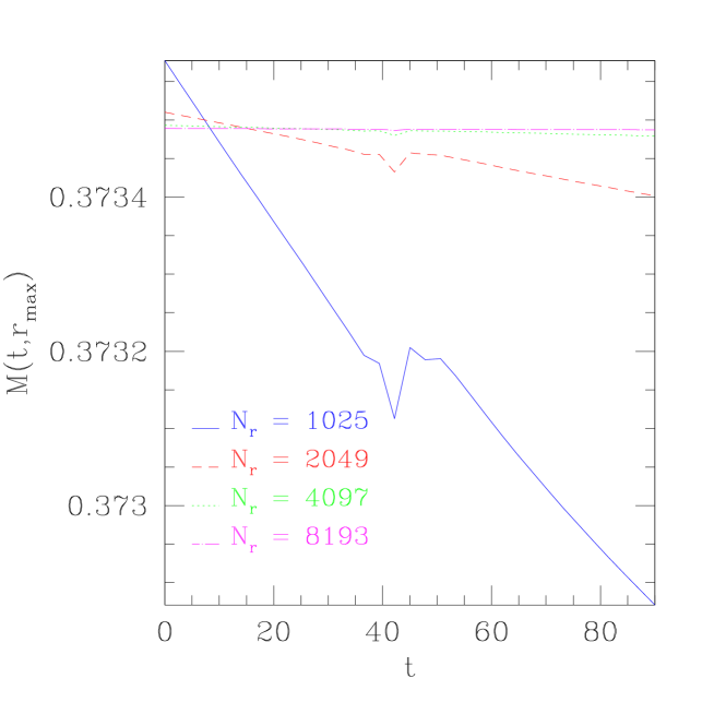
Figure 1: Convergence test of the spherically symmetric code. The estimated ADM mass, $M(t,r_{\rm max})$, is plotted against time, $t$, for four calculations using numbers of spatial grid points, $N_{r}$, of $1025,2049,4097$ and $8193$, so that the corresponding mesh spacings, $\Delta r$, are in a 8:4:2:1 ratio. The initial data parameters for the evolution are: $\phi_{0}=0.01$ for the complex field, and $A_{3}=0.001,r_{0}=40$ and $\sigma=3$ for the massless field (see (109)). The mass decreases with time in general, with a significant fluctuation at $40\leq t\leq 50$, when the real scalar field is close to the origin and strongly interacts with the boson star. The change in mass tends to vanish as we go to higher and higher resolutions. Combining results from the four calculations we find strong evidence that the finite difference scheme is second order accurate as expected.

Chapter 0

Transformation from Areal to Isotropic Spatial Coordinates

In this appendix we summarize the transformation from areal to isotropic spatial (radial) coordinates. This transformation can be used to generate boson stars initial data in isotropic coordinates from data computed in areal coordinates.

Using areal coordinates, the static, spherically-symmetric metric is

$$ds^{2}=-\alpha(R)^{2}dt^{2}+a(R)^{2}dR^{2}+R^{2}d\Omega^{2}\,,$$ (1)

while in isotropic coordinates it is

$$ds^{2}=-\alpha(r)^{2}dt^{2}+\psi(r)^{4}\left(dr^{2}+r^{2}d\Omega^{2}\right)\,.$$ (2)

We thus seek the spatial coordinate transformation

$$r=r(R)\,,$$ (3)

that leaves the $t$, $\theta$ and $\varphi$ coordinates unchanged. Comparing coefficients of $d\Omega^{2}$ and the two radial elements, we have

$$R^{2} = \psi^{4}r^{2}\,,$$ (4)

$$a^{2}dR^{2} = \psi^{4}dr^{2}\,,$$ (5)

which immediately yields

$$\psi = \sqrt{\frac{R}{r}}\,,$$ (6)

$$\frac{dr}{dR} = \pm\,a\frac{r}{R}\,.$$ (7)

Integrating the last equation, we have

$$r=C\exp\left(\pm\int\frac{a}{R}dR\right)\,,$$ (8)

where $C$ is some constant. The sign and the integration constant can be fixed by choosing $R\to r$ when $R\to\infty$:

$$\lim_{R\to\infty}\frac{r}{R}=1\,.$$ (9)

It is instructive to see the implication of the above by considering $R$ sufficiently large that the scalar field essentially vanishes. In vacuum the Schwarzschild metric (areal coordinates) takes the form

$$a^{2}=\left(1-\frac{2M}{R}\right)^{-1}\,,$$ (10)

where $M$ is the total mass inside the sphere of radius $R$. Expression (7) becomes

$$\frac{dr}{r}=\frac{dR}{\sqrt{R^{2}-2MR}}\,.$$ (11)

Integrating, we have

$$R=\frac{C^{\prime}r}{2}\left(1+\frac{M}{C^{\prime}r}\right)^{2}\,,$$ (12)

where $C^{\prime}$ is another integration constant. Applying the boundary condition (9) we have $C^{\prime}=2$, i.e.,

$$R=r\left(1+\frac{M}{2r}\right)^{2}\,.$$ (13)

Thus, in a vacuum region, we have

$$\alpha^{2} = 1-\frac{2M}{R}$$ (14)

$$= \left(\frac{1-M/2r}{1+M/2r}\right)^{2}\,,$$

and

$$\psi = \sqrt{\frac{R}{r}}$$ (15)

$$= 1+\frac{M}{2r}\,.$$

Therefore, in vacuum, we can write the metric as

$$ds^{2}=-\left(1-\frac{2M}{R}\right)dt^{2}+\left(1-\frac{2M}{R}\right)^{-1}dR^{2}+R^{2}d\Omega^{2}\,,$$ (16)

in Schwarzschild coordinates, and

$$ds^{2}=-\left(\frac{1-M/2r}{1+M/2r}\right)^{2}dt^{2}+\left(1+\frac{M}{2r}\right)^{4}\left(dr^{2}+r^{2}d\Omega^{2}\right)\,.$$ (17)

in isotropic coordinates.

From the above expression for the vacuum metric in isotropic coordinates we can rewrite $M$ in terms of $\psi$ and hence find

$$\alpha = \frac{1-M/2r}{1+M/2r}\,$$ (18)

$$= \frac{2}{\psi}-1\,.$$

Therefore in isotropic coordinates, the outer boundary condition for $\alpha$ is (82)

$$\lim_{r\to\infty}\alpha(r)=\frac{2}{\psi}-1\,.$$

If we have a numerical solution describing a boson star in areal coordinates, we can transform the solution to isotropic coordinates by numerically integrating (8) from the outer boundary inwards. In this case we need to express $r$ in terms of quantities known in the areal coordinate system. We may achieve this by noting that from (13) we have

$$r=\frac{R-M+\sqrt{R^{2}-2MR}}{2}\,.$$ (19)

On the other hand, in Schwarzschild coordinates we have

$$M=\frac{R}{2}\left(1-\frac{1}{a}\right)\,.$$ (20)

Substituting (20) in (19) we find

$$r=\left(\frac{1+\sqrt{a}}{2}\right)^{2}\frac{R}{a}\,.$$ (21)

In other words, the coordinate transformation from areal to isotropic coordinates is performed by solving

$$\left.r\,\right|_{R=R_{\mathrm{max}}} = \left[\left(\frac{1+\sqrt{a}}{2}\right)^{2}\frac{R}{a}\right]_{R=R_{\mathrm{max}}}\,,$$

$$\frac{dr}{dR} = \,a\frac{r}{R}\,.$$ (22)

On the other hand, under a coordinate transformation

$$\tilde{x}=\tilde{x}(x)\,,$$ (23)

we have

$${\tilde{g}_{\mu\nu}(\tilde{x})}=\frac{\partial{x}^{\alpha}}{\partial\tilde{x}^{\mu}}\frac{\partial{x}^{\beta}}{\partial\tilde{x}^{\nu}}g_{\alpha\beta}(x)\,.$$ (24)

Therefore, under the areal to isotropic coordinate transformation, we have

$$-\tilde{\alpha}(r)^{2}=\left[{\tilde{g}_{tt}}\right]_{\mathrm{I}}=\left[g_{tt}\right]_{\mathrm{A}}=-\alpha(R)^{2}\,,$$ (25)

where the subscripts I and A denote isotropic and areal respectively, and where quantities with (without) a tilde are functions of the isotropic (areal) radial coordinate. The above expression implies

$$\tilde{\alpha}(r(R))=\alpha(R)\,.$$ (26)

In other words, the lapse function transforms as a scalar under the specific transformation of areal to isotropic radial coordinates. If we now introduce a uniform grid in $R$

$$R_{i}=(i-1)\Delta R,\,\,\,i=1,\cdots,N+1$$ (27)

where $\Delta R=R_{\mathrm{max}}/N$, then after solving the initial value problem in areal coordinates, we have

$$\alpha_{i}\equiv\alpha(R_{i})=\tilde{\alpha}(r(R_{i}))\equiv\tilde{\alpha}(r_{i})\equiv\tilde{\alpha}_{i}\,,$$ (28)

where we have defined $\alpha_{i}$, $r_{i}$ and $\tilde{\alpha}_{i}$ by the above relations. Note that $\alpha_{i}$ is simply equal to $\tilde{\alpha}_{i}$, but that the latter is defined on a non-uniform grid $r_{i}\equiv r(R_{i})$ (whose values are obtained by solving the ODE (22)), and that therefore we need to do some interpolation if we want to express the function $\tilde{\alpha}$ on a grid that is uniform in $r$.

We can make an identical argument for the scalar field, $\phi$, to obtain the scalar field on the isotropic coordinate grid.

For the conformal factor $\psi$ we have

$$\tilde{\psi}(r)^{4}=\left[{\tilde{g}_{rr}}\right]_{\mathrm{I}}=\left(\frac{dR}{dr}\right)^{2}\left[g_{RR}\right]_{\mathrm{A}}=\left(\frac{dR}{dr}\right)^{2}a^{2}=\left(\frac{R}{r}\right)^{2}\,,$$ (29)

and therefore (we drop the tilde since $\psi$ is obviously defined in the isotropic coordinate system),

$$\psi(r)=\sqrt{\frac{R}{r(R)}}\,,$$ (30)

as it has to be. Hence on the non-uniform grid, $r_{i}$, we have

$$\psi_{i}\equiv\psi(r_{i})=\sqrt{\frac{R_{i}}{r(R_{i})}}=\sqrt{\frac{R_{i}}{r_{i}}}\,,$$ (31)

and, as before, we then need to do interpolation to obtain $\psi$ on a uniform isotropic grid.

Chapter 0

Numerical Determination of Spherical Boson Stars Using a Compactified Isotropic Coordinate

As described in Chap. A Numerical Study of Boson Stars, the system of equations that determines spherically symmetric boson stars is an eigenvalue problem. In this appendix we describe a numerical solution of this system that uses a compactified, isotropic radial coordinate.

Let $\phi(r)$, $\psi(r)$ and $\alpha(r)$ denote the modulus of the scalar field, the conformal factor, and the lapse function respectively. For notational simplicity let $\Phi\equiv\phi^{\prime}$, $\Psi\equiv\psi^{\prime}$, and $A\equiv\alpha^{\prime}$ denote the derivatives of the above functions with respect to $r$. The relevant system of equations can then be written as

$${\rm NewA}^{2}\phi+\left(\frac{A}{\alpha}+\frac{2\Psi}{\psi}\right)\Phi-\psi^{4}\left(m^{2}-\frac{\omega^{2}}{\alpha^{2}}\right)\phi = 0\,,$$ (1)

$${\rm NewA}^{2}\psi+\pi\left[\psi\Phi^{2}+\psi^{5}\left(\frac{\omega^{2}}{\alpha^{2}}+m^{2}\right)\phi^{2}\right] = 0\,,$$ (2)

$${\rm NewA}^{2}\alpha+\frac{2\Psi}{\psi}A-4\pi\psi^{4}\alpha\left(\frac{2\omega^{2}}{\alpha^{2}}-m^{2}\right)\phi^{2} = 0\,,$$ (3)

where ${\rm NewA}^{2}\equiv 3\frac{d}{dr^{3}}(r^{2}\frac{d}{dr})$. The regularity/boundary conditions are:

$$\Phi(0) = 0\,,$$ (4)

$$\Psi(0) = 0\,,$$ (5)

$$A(0) = 0\,,$$ (6)

$$\lim_{r\to\infty}\phi(r) = 0\,,$$ (7)

$$\lim_{r\to\infty}\psi(r) = 1\,,$$ (8)

$$\lim_{r\to\infty}\alpha(r) = 1\,.$$ (9)

We now perform a compactification of the spatial dimension by introducing a new coordinate, $\zeta$, such that

$$\zeta=\frac{r}{1+r}\,,$$ (10)

where $\zeta\in[0,1]$. Under the above transformation we have

$$r = \frac{\zeta}{1-\zeta}\,,$$ (11)

$$\frac{d}{dr} = (1-\zeta)^{2}\frac{d}{d\zeta}\,,$$ (12)

$${\rm NewA}^{2} = (1-\zeta)^{4}{\rm NewA}_{\zeta}^{2}\,,$$ (13)

where ${\rm NewA}_{\zeta}^{2}\equiv 3\frac{d}{d\zeta^{3}}(\zeta^{2}\frac{d}{d\zeta})$. The previous system of equations can be rewritten as

$${\rm NewA}_{\zeta}^{2}\phi+\left(\frac{A}{\alpha}+\frac{2\Psi}{\psi}\right)\Phi-\frac{\psi^{4}}{(1-\zeta)^{4}}\left(m^{2}-\frac{\omega^{2}}{\alpha^{2}}\right)\phi = 0\,,$$ (14)

$${\rm NewA}_{\zeta}^{2}\psi+\pi\left[\psi\Phi^{2}+\frac{\psi^{5}}{(1-\zeta)^{4}}\left(\frac{\omega^{2}}{\alpha^{2}}+m^{2}\right)\phi^{2}\right] = 0\,,$$ (15)

$${\rm NewA}_{\zeta}^{2}\alpha+\frac{2\Psi}{\psi}A-4\pi\frac{\psi^{4}\alpha}{(1-\zeta)^{4}}\left(\frac{2\omega^{2}}{\alpha^{2}}-m^{2}\right)\phi^{2} = 0\,,$$ (16)

with similar regularity/boundary conditions except that the $r\to\infty$ limit now becomes $\zeta\to 1$. A second order finite difference form of the above equations is

$$3\Delta^{{}^{\scriptstyle\frac{r^{3}}{2}}}_{{}_{\scriptstyle 0}}\left(r_{{}_{\scriptstyle j}}^{2}\,\Delta^{{}^{\scriptstyle\frac{r}{2}}}_{{}_{\scriptstyle 0}}\phi^{{}^{\scriptstyle n}}_{{}_{\scriptstyle j}}\right)+\left(\frac{\Delta^{{}^{\scriptstyle r}}_{{}_{\scriptstyle 0}}\alpha^{{}^{\scriptstyle n}}_{{}_{\scriptstyle j}}}{\alpha^{{}^{\scriptstyle n}}_{{}_{\scriptstyle j}}}+\frac{2\Delta^{{}^{\scriptstyle r}}_{{}_{\scriptstyle 0}}\psi^{{}^{\scriptstyle n}}_{{}_{\scriptstyle j}}}{\psi^{{}^{\scriptstyle n}}_{{}_{\scriptstyle j}}}\right)\Delta^{{}^{\scriptstyle r}}_{{}_{\scriptstyle 0}}\phi^{{}^{\scriptstyle n}}_{{}_{\scriptstyle j}}-\frac{{\psi^{{}^{\scriptstyle n}}_{{}_{\scriptstyle j}}}^{4}}{(1-r_{j})^{4}}\left(m^{2}-\frac{\omega^{2}}{{\alpha^{{}^{\scriptstyle n}}_{{}_{\scriptstyle j}}}^{2}}\right)\phi^{{}^{\scriptstyle n}}_{{}_{\scriptstyle j}} = 0\,,\;\;\;\;$$ (17)

$$3\Delta^{{}^{\scriptstyle\frac{r^{3}}{2}}}_{{}_{\scriptstyle 0}}\left(r_{{}_{\scriptstyle j}}^{2}\,\Delta^{{}^{\scriptstyle\frac{r}{2}}}_{{}_{\scriptstyle 0}}\psi^{{}^{\scriptstyle n}}_{{}_{\scriptstyle j}}\right)+\pi\left[\psi^{{}^{\scriptstyle n}}_{{}_{\scriptstyle j}}\left(\Delta^{{}^{\scriptstyle r}}_{{}_{\scriptstyle 0}}\phi^{{}^{\scriptstyle n}}_{{}_{\scriptstyle j}}\right)^{2}+\frac{{\psi^{{}^{\scriptstyle n}}_{{}_{\scriptstyle j}}}^{5}}{(1-r_{j})^{4}}\left(\frac{\omega^{2}}{{\alpha^{{}^{\scriptstyle n}}_{{}_{\scriptstyle j}}}^{2}}+m^{2}\right){\phi^{{}^{\scriptstyle n}}_{{}_{\scriptstyle j}}}^{2}\right] = 0\,,\;\;\;\;$$ (18)

$$3\Delta^{{}^{\scriptstyle\frac{r^{3}}{2}}}_{{}_{\scriptstyle 0}}\left(r_{{}_{\scriptstyle j}}^{2}\,\Delta^{{}^{\scriptstyle\frac{r}{2}}}_{{}_{\scriptstyle 0}}\alpha^{{}^{\scriptstyle n}}_{{}_{\scriptstyle j}}\right)+\frac{2\Delta^{{}^{\scriptstyle r}}_{{}_{\scriptstyle 0}}{\psi^{{}^{\scriptstyle n}}_{{}_{\scriptstyle j}}}}{\psi^{{}^{\scriptstyle n}}_{{}_{\scriptstyle j}}}\Delta^{{}^{\scriptstyle r}}_{{}_{\scriptstyle 0}}\alpha^{{}^{\scriptstyle n}}_{{}_{\scriptstyle j}}-4\pi\frac{{\psi^{{}^{\scriptstyle n}}_{{}_{\scriptstyle j}}}^{4}\alpha^{{}^{\scriptstyle n}}_{{}_{\scriptstyle j}}}{(1-r_{j})^{4}}\left(\frac{2\omega^{2}}{{\alpha^{{}^{\scriptstyle n}}_{{}_{\scriptstyle j}}}^{2}}-m^{2}\right){\phi^{{}^{\scriptstyle n}}_{{}_{\scriptstyle j}}}^{2} = 0\,,\;\;\;\;$$ (19)

for $j=2,\cdots,N_{r}-1$.

The discrete regularity/boundary conditions are

$$\phi^{{}^{\scriptstyle n}}_{{}_{\scriptstyle 1}} = \frac{4\phi^{{}^{\scriptstyle n}}_{{}_{\scriptstyle 2}}-\phi^{{}^{\scriptstyle n}}_{{}_{\scriptstyle 3}}}{3}\,,$$ (20)

$$\phi^{{}^{\scriptstyle n}}_{{}_{\scriptstyle N_{r}}} = 0\,,$$ (21)

with similar equations for $\psi^{{}^{\scriptstyle n}}_{{}_{\scriptstyle j}}$ and $\alpha^{{}^{\scriptstyle n}}_{{}_{\scriptstyle j}}$.

Equation (17) is linear in $\phi$ and is viewed as an eigenvalue equation with eigenvalue $-\omega^{2}$ and eigenvector $\phi$. More specifically, (17) can be written as a matrix equation

$$\sum_{j}L_{i,j}\phi_{j}=-\omega^{2}\phi_{j}\,,$$ (22)

where $L_{i,j}$ is a tridiagonal matrix. The matrix $L_{i,j}$ is in general not symmetric. Transformation to a symmetric tridiagonal form can be performed using the FIGI routine in the EISPACK [94] package, and then (22) can be solved with the symmetric tridiagonal eigenvalue solver RATQR and TINVIT from the same package. Equation (18) is non-linear in $\psi_{j}$ and is solved by a global Newton method, with each Newton step involving a tridiagonal linear solve. Finally, (19) can also be solved for $\alpha_{j}$ using a tridiagonal solver. The sequence of solving (17), (18) and (19) is repeated until the total change in the variables from iteration to iteration is within a prescribed tolerance, typically chosen to be $\epsilon=10^{-10}$.

Chapter 0

Summary of Equations for Stationary, Axisymmetric Boson Stars and Associated Finite Difference Formulae

In this appendix we give a summary of the system of equations (System A of Chap. A Numerical Study of Boson Stars) that determines stationary, rotating, axisymmetric boson stars in quasi-isotropic coordinates, as well as our finite difference approximation of the system.

The spacetime metric is written as

$$ds^{2}=\left(-\alpha^{2}+\psi^{4}r^{2}\sin^{2}\theta e^{2\sigma}\beta^{2}\right)dt^{2}+\psi^{4}\left(dr^{2}+r^{2}d\theta^{2}+r^{2}\sin^{2}\theta e^{2\sigma}d\varphi^{2}\right)+2\psi^{4}r^{2}\sin^{2}\theta e^{2\sigma}\beta dtd\varphi$$ (1)

and the equations for the five unknown functions $\alpha,\beta,\psi,\sigma$ and $\phi$ (which depend on $r$ and $\theta$ only) are

$$\begin{split}\phi_{,rr}+\frac{2}{r}\phi_{,r}+\frac{1}{r^{2}}\phi_{,\theta\theta}+\frac{\cot\theta}{r^{2}}\phi_{,\theta}-\frac{k^{2}}{r^{2}\sin^{2}\theta e^{2\sigma}}\phi+\left(\sigma_{,r}+\frac{\alpha_{,r}}{\alpha}+\frac{2\psi_{,r}}{\psi}\right)\phi_{,r}\\ +\left(\sigma_{,\theta}+\frac{\alpha_{,\theta}}{\alpha}+\frac{2\psi_{,\theta}}{\psi}\right)\frac{\phi_{,\theta}}{r^{2}}+\left[\left(\frac{\omega-\beta k}{\alpha}\right)^{2}-m^{2}\right]\psi^{4}\phi=0\,,\end{split}$$ (2)

$$\psi_{,rr}+\frac{\psi_{,\theta\theta}}{r^{2}}+\left(\frac{1}{r}-\frac{\alpha_{,r}}{\alpha}-\frac{\psi_{,r}}{\psi}\right)\psi_{,r}-\left(\frac{\psi_{,\theta}}{\psi}+\frac{\alpha_{,\theta}}{\alpha}\right)\frac{\psi_{,\theta}}{r^{2}}-\frac{\psi^{5}r^{2}\sin^{2}\theta e^{2\sigma}}{8\alpha^{2}}\left(\beta_{,r}\,^{2}+\frac{\beta_{,\theta}\,^{2}}{r^{2}}\right)$$

$$-\frac{\psi}{2r}\left[\left(1+r\sigma_{,r}\right)\frac{\alpha_{,r}}{\alpha}+\frac{1}{r}\left(\cot\theta+\sigma_{,\theta}\right)\frac{\alpha_{\theta}}{\alpha}\right]=$$

$$-2\pi\psi\left[\left(\phi_{,r}\,^{2}+\frac{\phi_{,\theta}\,^{2}}{r^{2}}\right)+\phi^{2}\left(\frac{\psi^{4}}{\alpha^{2}}(w-\beta k)^{2}-\frac{k^{2}}{r^{2}\sin^{2}\theta e^{2\sigma}}\right)\right]\,,$$ (3)

$$\beta_{,rr}+\frac{\beta_{,\theta\theta}}{r^{2}}+\left(\frac{4}{r}+3\sigma_{,r}-\frac{\alpha_{,r}}{\alpha}+6\frac{\psi_{,r}}{\psi}\right)\beta_{,r}+\left(3\cot\theta+3\sigma_{,\theta}-\frac{\alpha_{,\theta}}{\alpha}+6\frac{\psi_{,\theta}}{\psi}\right)\frac{\beta_{,\theta}}{r^{2}}=-16\pi\phi^{2}\frac{k(\omega-\beta k)}{r^{2}\sin^{2}\theta e^{2\sigma}}\,,$$ (4)

$$\begin{split}\alpha_{,rr}+\frac{2}{r}\alpha_{,r}+\frac{1}{r^{2}}\alpha_{,\theta\theta}+\frac{\cot\theta}{r^{2}}\alpha_{,\theta}+\left(\frac{2\psi_{,r}}{\psi}+\sigma_{,r}\right)\alpha_{,r}+\left(2\frac{\psi_{,\theta}}{\psi}+\sigma_{,\theta}\right)\frac{\alpha_{,\theta}}{r^{2}}\\ -\frac{\psi^{4}r^{2}\sin^{2}\theta e^{2\sigma}}{2\alpha}\left(\beta_{,r}\,^{2}+\frac{\beta_{,\theta}\,^{2}}{r^{2}}\right)+4\pi\alpha\psi^{4}\phi^{2}\left(m^{2}-\frac{2(\omega-\beta k)^{2}}{\alpha^{2}}\right)=0\,,\end{split}$$ (5)

$$\begin{split}\sigma_{,rr}+\frac{\sigma_{,\theta\theta}}{r^{2}}+\left(\sigma_{,r}+4\frac{\psi_{,r}}{\psi}+\frac{2\alpha_{,r}}{\alpha}+\frac{3}{r}\right)\sigma_{,r}+\left(\sigma_{,\theta}+4\frac{\psi_{,\theta}}{\psi}+\frac{2\alpha_{,\theta}}{\alpha}+2\cot\theta\right)\frac{\sigma_{,\theta}}{r^{2}}\\ +\frac{4}{\psi}\left[\left(\frac{\psi_{,r}}{\psi}+\frac{\alpha_{,r}}{\alpha}+\frac{1}{r}\right)\psi_{,r}+\left(\frac{\psi_{,\theta}}{\psi}+\frac{\alpha_{,\theta}}{\alpha}+\cot\theta\right)\frac{\psi_{,\theta}}{r^{2}}\right]+\frac{2}{\alpha r}\left(\alpha_{,r}+\cot\theta\frac{\alpha_{,\theta}}{r}\right)\\ +\frac{3\psi^{4}r^{2}\sin^{2}\theta e^{2\sigma}}{4\alpha^{2}}\left(\beta_{,r}\,^{2}+\frac{\beta_{,\theta}\,^{2}}{r^{2}}\right)\\ +4\pi\left[\left(m^{2}+\frac{3k^{2}}{\psi^{4}r^{2}\sin^{2}\theta e^{2\sigma}}-\left(\frac{\omega-\beta k}{\alpha}\right)^{2}\right)\phi^{2}\psi^{4}-\left(\phi_{,r}^{2}+\frac{\phi_{,\theta}^{2}}{r^{2}}\right)\right]=0\,.\end{split}$$ (6)

With the coordinate transformation

$$\zeta = \frac{r}{1+r}\,,$$ (7)

$$s = \cos\theta\,,$$ (8)

the equations become

$$\left(\frac{1-\zeta}{\zeta}\right)^{2}\left[3\zeta^{2}\left(1-\zeta\right)^{2}\left(\zeta^{2}\phi_{,\zeta}\right)_{,\zeta^{3}}+\left((1-s^{2})\phi_{,s}\right)_{,s}-\frac{k^{2}}{\left(1-s^{2}\right)e^{2\sigma}}\phi\right]+$$

$$\left(1-\zeta\right)^{4}\left(\sigma_{,\zeta}+\frac{\alpha_{,\zeta}}{\alpha}+\frac{2\psi_{,\zeta}}{\psi}\right)\phi_{,\zeta}+\left(\frac{1-\zeta}{\zeta}\right)^{2}\left(1-s^{2}\right)\left(\sigma_{,s}+\frac{\alpha_{,s}}{\alpha}+\frac{2\psi_{,s}}{\psi}\right)\phi_{,s}$$

$$\hskip 199.16928pt+\left[\left(\frac{\omega-\beta k}{\alpha}\right)^{2}-m^{2}\right]\psi^{4}\phi=0\,,$$ (9)

$$\left(\frac{1-\zeta}{\zeta}\right)^{2}\left[3\zeta^{2}\left(1-\zeta\right)^{2}\left(\zeta^{2}\psi_{,\zeta}\right)_{,\zeta^{3}}+(1-s^{2})\psi_{,ss}-s\psi_{,s}\right]$$

$$-\left(1-\zeta\right)^{3}\left[\frac{1}{\zeta}+(1-\zeta)\left(\frac{\alpha_{,\zeta}}{\alpha}+\frac{\psi_{,\zeta}}{\psi}\right)\right]\psi_{,\zeta}$$

$$-(1-s^{2})\left(\frac{1-\zeta}{\zeta}\right)^{2}\left(\frac{\psi_{,s}}{\psi}+\frac{\alpha_{,s}}{\alpha}\right)\psi_{,s}$$

$$-\frac{\psi^{5}\zeta^{2}(1-s^{2})e^{2\sigma}}{8\alpha^{2}}\left[(1-\zeta)^{2}\beta_{,\zeta}\,^{2}+\frac{1}{\zeta^{2}}(1-s^{2})\beta_{,s}\,^{2}\right]$$

$$-\frac{\psi}{2\alpha}\left(\frac{1-\zeta}{\zeta}\right)\left[(1-\zeta)^{2}\left(1+\zeta(1-\zeta)\sigma_{,\zeta}\right)\alpha_{,\zeta}+\left(\frac{1-\zeta}{\zeta}\right)\left((1-s^{2})\sigma_{,s}-s\right)\alpha_{,s}\right]$$

$$+2\pi\psi\left[(1-\zeta)^{4}{\phi_{,\zeta}}^{2}+\left(\frac{1-\zeta}{\zeta}\right)^{2}(1-s^{2}){\phi_{,s}}^{2}+\right.$$

$$\left.\phi^{2}\left(\frac{\psi^{4}}{\alpha^{2}}(\omega-\beta k)^{2}-\frac{k^{2}(1-\zeta)^{2}}{\zeta^{2}(1-s^{2})e^{2\sigma}}\right)\right]=0\,,$$ (10)

$$\left(\frac{1-\zeta}{\zeta}\right)^{2}\left\{3\zeta^{2}\left(1-\zeta\right)^{2}\left(\zeta^{2}\beta_{,\zeta}\right)_{,\zeta^{3}}+\left[\left(1-s^{2}\right)\beta_{,ss}-s\beta_{,s}\right]\right\}$$

$$+\left(1-\zeta\right)^{3}\left[\frac{2}{\zeta}+\left(1-\zeta\right)\left(3\sigma_{,\zeta}-\frac{\alpha_{,\zeta}}{\alpha}+6\frac{\psi_{,\zeta}}{\psi}\right)\right]\beta_{,\zeta}$$

$$+\left(\frac{1-\zeta}{\zeta}\right)^{2}\left[-3s+\left(1-s^{2}\right)\left(3\sigma_{,s}-\frac{\alpha_{,s}}{\alpha}+6\frac{\psi_{,s}}{\psi}\right)\right]\beta_{,s}$$

$$+16\pi\frac{k\left(\omega-\beta k\right)}{\left(1-s^{2}\right)e^{2\sigma}}\left(\frac{1-\zeta}{\zeta}\right)^{2}\phi^{2}=0\,,$$ (11)

$$\left(\frac{1-\zeta}{\zeta}\right)^{2}\left[3\zeta^{2}\left(1-\zeta\right)^{2}\left(\zeta^{2}\alpha_{,\zeta}\right)_{,\zeta^{3}}+(1-s^{2})\alpha_{,ss}-s\alpha_{,s}\right]+\left(1-\zeta\right)^{4}\left(\frac{2\psi_{,\zeta}}{\psi}+\sigma_{,\zeta}\right)\alpha_{,\zeta}$$

$$+\left(\frac{1-\zeta}{\zeta}\right)^{2}\left[-s+(1-s^{2})\left(\frac{2\psi_{,s}}{\psi}+\sigma_{,s}\right)\right]\alpha_{,s}$$

$$-\psi^{4}\frac{(1-s^{2})e^{2\sigma}}{2\alpha}\left[\zeta^{2}\left(1-\zeta\right)^{2}{\beta_{,\zeta}}^{2}+(1-s^{2}){\beta_{,s}}^{2}\right]+$$

$$4\pi\alpha\psi^{4}\phi^{2}\left[m^{2}-\frac{2\left(\omega-\beta k\right)^{2}}{\alpha^{2}}\right]=0\,,$$ (12)

$$\left(\frac{1-\zeta}{\zeta}\right)^{2}\left\{3\zeta^{2}\left(1-\zeta\right)^{2}\left(\zeta^{2}\sigma_{,\zeta}\right)_{,\zeta^{3}}+\left[\left(1-s^{2}\right)\sigma_{,ss}-s\sigma_{,s}\right]\right\}$$

$$+\left(1-\zeta\right)^{3}\left[\left(1-\zeta\right)\left(\sigma_{,\zeta}+4\frac{\psi_{,\zeta}}{\psi}+2\frac{\alpha_{,\zeta}}{\alpha}\right)+\frac{1}{\zeta}\right]\sigma_{,\zeta}$$

$$+\left(\frac{1-\zeta}{\zeta}\right)^{2}\left[(1-s^{2})\left(\sigma_{,s}+4\frac{\psi_{,s}}{\psi}+2\frac{\alpha_{s}}{\alpha}\right)-2s\right]\sigma_{,s}$$

$$+\frac{4}{\psi}\left\{\left(1-\zeta\right)^{3}\left[(1-\zeta)\left(\frac{\psi_{,\zeta}}{\psi}+\frac{\alpha_{,\zeta}}{\alpha}\right)+\frac{1}{\zeta}\right]\psi_{,\zeta}\right.$$

$$\left.+\left(\frac{1-\zeta}{\zeta}\right)^{2}\left[(1-s^{2})\left(\frac{\psi_{,s}}{\psi}+\frac{\alpha_{,s}}{\alpha}\right)-s\right]\psi_{,s}\right\}$$

$$+\frac{2}{\alpha}\frac{(1-\zeta)^{2}}{\zeta}\left[\left(1-\zeta\right)\alpha_{,\zeta}-\frac{s}{\zeta}\alpha_{,s}\right]+\frac{3\psi^{4}(1-s^{2})e^{2\sigma}}{4\alpha^{2}}\left[\zeta^{2}(1-\zeta)^{2}{\beta_{,\zeta}}^{2}+(1-s^{2}){\beta_{,s}}^{2}\right]$$

$$+4\pi\left\{\left[m^{2}+\frac{3k^{2}}{\psi^{4}(1-s^{2})e^{2\sigma}}\left(\frac{1-\zeta}{\zeta}\right)^{2}-\left(\frac{\omega-\beta k}{\alpha}\right)^{2}\right]\phi^{2}\psi^{4}-\right.$$

$$\left.\left[\left(1-\zeta\right)^{4}{\phi_{,\zeta}}^{2}+\left(\frac{1-\zeta}{\zeta}\right)^{2}(1-s^{2}){\phi_{,s}}^{2}\right]\right\}\,.$$ (13)

The regularity conditions for the system at $\zeta=0$ are given by

$$\phi(0,s) = 0\,,$$ (14)

$$\psi_{,\zeta}(0,s) = 0\,,$$ (15)

$$\beta_{,\zeta}(0,s) = 0\,,$$ (16)

$$\alpha_{,\zeta}(0,s) = 0\,,$$ (17)

$$\sigma(0,s) = 0\,,$$ (18)

and boundary conditions at $\zeta=1$ are

$$\phi(1,s) = 0\,,$$ (19)

$$\psi(1,s) = 1\,,$$ (20)

$$\beta(1,s) = 0\,,$$ (21)

$$\alpha(1,s) = 1\,,$$ (22)

$$\sigma(1,s) = 0\,.$$ (23)

The boundary conditions at $s=0$ (the equatorial plane) are

$$\phi_{,s}(\zeta,0) = 0\,,$$ (24)

$$\psi_{,s}(\zeta,0) = 0\,,$$ (25)

$$\beta_{,s}(\zeta,0) = 0\,,$$ (26)

$$\alpha_{,s}(\zeta,0) = 0\,,$$ (27)

$$\sigma_{,s}(\zeta,0) = 0\,,$$ (28)

while at $s=1$ (the axis of symmetry), we have

$$\phi(\zeta,1) = 0\,,$$ (29)

$$\psi_{,s}(\zeta,1) = 0\,,$$ (30)

$$\beta_{,s}(\zeta,1) = 0\,,$$ (31)

$$\alpha_{,s}(\zeta,1) = 0\,,$$ (32)

$$\sigma_{,s}(\zeta,1) = 0\,.$$ (33)

For the finite difference formulae, since the expressions are lengthy and messy, we simply note that we extend the difference operators defined in App. A Numerical Study of Boson Stars to operators acting in two spatial dimensions in the obvious way. More explicitly, we will have

$$\Delta^{{}^{\zeta}}_{{}_{0}}u_{{}_{{\scriptstyle i},{\scriptstyle j}}} \equiv \frac{u_{{}_{{\scriptstyle i}+1,{\scriptstyle j}}}-u_{{}_{{\scriptstyle i}-1,{\scriptstyle j}}}}{2\Delta\zeta}$$

$${\Delta^{{}^{\scriptstyle s}}_{{}_{\scriptstyle 0}}}u_{{}_{{\scriptstyle i},{\scriptstyle j}}} \equiv \frac{u_{{}_{{\scriptstyle i},{\scriptstyle j}+1}}-u_{{}_{{\scriptstyle i},{\scriptstyle j}-1}}}{2\Delta s}$$

etc..

The difference equations are then obtained by performing the following substitutions in (9)-(13):

$$\frac{\partial}{\partial\zeta^{3}} \longrightarrow \Delta^{{}^{\scriptstyle\zeta^{3}}}_{{}_{\scriptstyle 0}}\,,$$

$$\frac{\partial}{\partial\zeta} \longrightarrow \Delta^{{}^{\scriptstyle\zeta}}_{{}_{\scriptstyle 0}}\,,$$

$$\frac{\partial^{2}}{\partial s^{2}} \longrightarrow \Delta^{{}^{\scriptstyle s}}_{{}_{\scriptstyle+}}\Delta^{{}^{\scriptstyle s}}_{{}_{\scriptstyle-}}\,,$$

$$\frac{\partial}{\partial s} \longrightarrow \Delta^{{}^{\scriptstyle s}}_{{}_{\scriptstyle 0}}\,.$$

Chapter 0

Weak Field Limit: Derivation of the Poisson-Schrödinger system from the Einstein-Klein-Gordon System

In this appendix we will consider the weak field limit (Newtonian limit) of the Einstein-Klein-Gordon (EKG) system—thereby deriving the Poisson-Schrödinger (PS) system, which represents non-relativistic Newtonian boson stars—with all approximations explicitly stated. The main purpose of this derivation is to provide the background for checking whether the stationary Newtonian solutions obtained by solving the PS system provide good initial estimates for the algorithm used to determine the stationary general relativistic solutions (see Sec. 0.20.3). The assumptions made in deriving the Newtonian limit that need to be checked on a solution-by-solution basis will be summarized at the end of the appendix.

Note that here we write the equations for the EKG system as:

$$G_{\alpha\beta}=\kappa T_{\alpha\beta}\,,\\$$ (1)

$${\rm NewA}^{\alpha}{\rm NewA}_{\alpha}\phi-m^{2}\phi=0\,,$$ (2)

where $\kappa$ is a constant which is conventionally chosen to be $8\pi$.

Appendix A Poisson Equation

The derivation of the Poisson equation for the Newtonian gravitational potential from the Einstein field equation is quite standard [95, 89], although the right hand side of the equation (matter coupling) is usually not worked out in detail, and the order of truncation is often not clearly stated. We suppose that spacetime is nearly flat. The metric can then be written as

$$g_{\alpha\beta}=\eta_{\alpha\beta}+h_{\alpha\beta}\,,$$ (3)

where

$$|h_{\alpha\beta}|=O(\epsilon)\ll 1\,,$$ (4)

and $\eta_{\alpha\beta}$ is the flat metric in Cartesian coordinates $\eta=\mathrm{diag}\left(-1,1,1,1\right)$.  There are two classes of coordinate transformations which preserve the above form: the background Lorentz transformations and gauge transformations [95]. Gauge transformations can be written in the form

$$x^{\bar{\alpha}}=x^{\alpha}+\xi^{\alpha}(x^{\beta})\,,$$ (5)

where

$$|\xi^{\alpha}\,_{,\beta}|=O(\epsilon)\,.$$ (6)

The Jacobian matrix associated with (5) can be written as

$$\Lambda^{\bar{\alpha}}\,_{\beta}=\delta^{\alpha}\,_{\beta}+\xi^{\alpha}\,_{,\beta}\,,$$ (7)

with an inverse given by

$$\Lambda^{\alpha}\,_{\bar{\beta}}=\delta^{\alpha}\,_{\beta}-\xi^{\alpha}\,_{,\beta}+O(\epsilon^{2})\,,$$ (8)

as is established by the following:

$$\Lambda^{\bar{\alpha}}\,_{\beta}\,\Lambda^{\beta}\,_{\bar{\gamma}} = (\delta^{\alpha}\,_{\beta}+\xi^{\alpha}\,_{,\beta})(\delta^{\beta}\,_{\gamma}-\xi^{\beta}\,_{,\gamma})$$ (9)

$$= \delta^{\alpha}\,_{\gamma}+\xi^{\alpha}\,_{,\gamma}-\xi^{\alpha}\,_{,\gamma}+\xi^{\alpha}\,_{,\beta}\,\xi^{\beta}\,_{,\gamma}$$

$$= \delta^{\alpha}\,_{\gamma}+O(\epsilon^{2})\,.$$

Now

$$g_{\bar{\alpha}\bar{\beta}} = \Lambda^{\mu}\,_{\bar{\alpha}}\Lambda^{\nu}\,_{\bar{\beta}}\,g_{\mu\nu}$$ (10)

$$= \Lambda^{\mu}\,_{\bar{\alpha}}\Lambda^{\nu}\,_{\bar{\beta}}\,\eta_{\mu\nu}+\Lambda^{\mu}\,_{\bar{\alpha}}\Lambda^{\nu}\,_{\bar{\beta}}\,h_{\mu\nu}$$

$$= (\delta^{\mu}\,_{\alpha}-\xi^{\mu}\,_{,\alpha})(\delta^{\nu}\,_{\beta}-\xi^{\nu}\,_{,\beta})\,\eta_{\mu\nu}+(\delta^{\mu}\,_{\alpha}-\xi^{\mu}\,_{,\alpha})(\delta^{\nu}\,_{\beta}-\xi^{\nu}\,_{,\beta})\,h_{\mu\nu}+O(\epsilon^{2})$$

$$= \eta_{\alpha\beta}-\xi^{\mu}\,_{,\alpha}\,\eta_{\mu\beta}-\xi^{\nu}\,_{,\beta}\,\eta_{\alpha\nu}+h_{\alpha\beta}+O(\epsilon^{2})$$

$$= \eta_{\alpha\beta}+h_{\alpha\beta}-\xi_{\alpha,\beta}-\xi_{\beta,\alpha}+O(\epsilon^{2})\,,$$

or

$$h_{\bar{\alpha}\bar{\beta}}=h_{\alpha\beta}-\xi_{\alpha,\beta}-\xi_{\beta,\alpha}+O(\epsilon^{2})\,,$$ (11)

where in the last step we have adopted the notational convention that we lower and raise tensor indices using $\eta_{\alpha\beta}$. That is, $h^{\alpha\beta}$ is, by definition, $\eta^{\alpha\mu}\eta^{\beta\nu}h_{\mu\nu}$. (Note that using this convention we also have $g^{\alpha\beta}=\eta^{\alpha\beta}-h^{\alpha\beta}+O(\epsilon^{2})$. In other words, for all quantities of order $O(\epsilon)$, raising and lowering of indices using $\eta$ rather than $g$ will lead to deviations of order $O(\epsilon^{2})$. )

By definition, we have

$$-R^{\alpha}\,_{\beta\mu\nu}=\Gamma^{\alpha}\,_{\beta\mu,\nu}-\Gamma^{\alpha}\,_{\beta\nu,\mu}+\Gamma^{\alpha}\,_{\sigma\nu}\,\Gamma^{\sigma}\,_{\beta\mu}-\Gamma^{\alpha}\,_{\sigma\mu}\,\Gamma^{\sigma}\,_{\beta\nu}\,,$$ (12)

where

$$\Gamma^{\lambda}\,_{\mu\nu}=\frac{1}{2}\eta^{\lambda\rho}\left(h_{\rho\nu,\mu}+h_{\mu\rho,\nu}-h_{\mu\nu,\rho}\right)+O(\epsilon^{2})\,.$$ (13)

Note that we have used the fact that we work in Cartesian coordinates (and hence that the derivatives of $\eta$ vanish), and that we assume that derivatives of small numbers are also small

$$h_{\alpha\beta,\gamma}=O(\epsilon)\,$$ (14)

(so that we can drop terms such as $h^{\alpha\beta}h_{\beta\gamma,\delta}$).

Now we have

$$R^{\alpha}\,_{\beta\mu\nu}=-\frac{1}{2}\eta^{\alpha\rho}\left(h_{\rho\mu,\beta\nu}+h_{\beta\rho,\mu\nu}-h_{\beta\mu,\rho\nu}\right)-\left(\mu\leftrightarrow\nu\right)+O(\epsilon^{2})\,.$$ (15)

The second terms within parentheses in the above cancel, so that we have

$$R_{\alpha\beta\mu\nu}=\frac{1}{2}\left(h_{\alpha\nu,\beta\mu}-h_{\beta\nu,\alpha\mu}-h_{\alpha\mu,\beta\nu}+h_{\beta\mu,\alpha\nu}\right)+O(\epsilon^{2})\,,$$ (16)

and

$$R_{\beta\nu} = \frac{1}{2}\left(h^{\mu}\,_{\nu,\beta\mu}-h_{\beta\nu,\mu}\,^{\mu}-h^{\mu}\,_{\mu,\beta\nu}+h_{\beta\mu,}\,^{\mu}\,{}_{\nu}\right)+O(\epsilon^{2})$$ (17)

$$= \frac{1}{2}\left(h^{\mu}\,_{\nu,\beta\mu}-\Box h_{\beta\nu}-h\,_{,\beta\nu}+h_{\beta\mu,}\,^{\mu}\,{}_{\nu}\right)+O(\epsilon^{2})\,,$$

and

$$R=\left(h_{\mu\nu,}\,^{\mu\nu}-\Box h\right)+O(\epsilon^{2})\,,$$ (18)

where we have defined $h\equiv h^{\mu}\,_{\mu}$ and $\Box h\equiv h_{,\mu}\,^{\mu}$.

Constructing the Einstein tensor, we then have

$$R_{\beta\nu}-\frac{1}{2}\eta_{\beta\nu}R=\frac{1}{2}\left(h^{\mu}\,_{\nu,\beta\mu}-\Box h_{\beta\nu}-h\,_{,\beta\nu}+h_{\beta\mu,}\,^{\mu}\,{}_{\nu}-\eta_{\beta\nu}h_{\gamma\delta,}\,^{\gamma\delta}+\eta_{\beta\nu}\Box h\right)+O(\epsilon^{2})\,.$$ (19)

If we define

$$\bar{h}^{\alpha\beta}\equiv h^{\alpha\beta}-\frac{1}{2}\eta^{\alpha\beta}h\,,$$ (20)

then

$$\bar{h}=-h\,,$$ (21)

and

$$h^{\alpha\beta}=\bar{h}^{\alpha\beta}-\frac{1}{2}\eta^{\alpha\beta}\bar{h}\,.$$ (22)

Now

$$G_{\beta\nu} = \frac{1}{2}\left(\bar{h}^{\mu}\,_{\nu,\beta\mu}-\frac{1}{2}\bar{h}_{,\beta\nu}-\Box\bar{h}_{\beta\nu}+\frac{1}{2}\eta_{\beta\nu}\Box\bar{h}+\bar{h}_{,\beta\nu}+\bar{h}_{\beta\mu,}\,^{\mu}\,{}_{\nu}-\frac{1}{2}\bar{h}_{,\beta\nu}-\eta_{\beta\nu}\bar{h}_{\gamma\delta,}\,^{\gamma\delta}\right.$$ (23)

$$\left.+\frac{1}{2}\eta_{\beta\nu}\Box\bar{h}-\eta_{\beta\nu}\Box\bar{h}\right)+O(\epsilon^{2})$$

$$= \frac{1}{2}\left(-\Box\bar{h}_{\beta\nu}+\bar{h}^{\mu}\,_{\nu,\beta\mu}+\bar{h}_{\beta\mu,}\,^{\mu}\,{}_{\nu}-\eta_{\beta\nu}\bar{h}_{\gamma\delta,}\,^{\gamma\delta}\right)+O(\epsilon^{2})\,.$$

If we now impose the Lorentz (or harmonic) gauge condition

$$\bar{h}^{\mu\nu}\,_{,\nu}=0\,,$$ (24)

we have

$$G_{\alpha\beta}=-\frac{1}{2}\Box\bar{h}_{\alpha\beta}+O(\epsilon^{2})\,,$$ (25)

and hence

$$\Box\bar{h}_{\alpha\beta}=-2\kappa T_{\alpha\beta}+O(\epsilon^{2})\,.$$ (26)

The existence of the Lorentz gauge can be shown as follows. From (11) it follows that

$$h^{\bar{\alpha}}\,_{\bar{\alpha}}=h-2\xi^{\alpha},_{\alpha}+O(\epsilon^{2})\,.$$ (27)

Also, we have

$$\bar{h}_{\bar{\alpha}\bar{\beta}} = h_{\bar{\alpha}\bar{\beta}}-\frac{1}{2}\eta_{\bar{\alpha}\bar{\beta}}h^{\bar{\gamma}}\,_{\bar{\gamma}}$$ (28)

$$= h_{\alpha\beta}-\xi_{\alpha,\beta}-\xi_{\beta,\alpha}-\frac{1}{2}\eta_{\alpha\beta}(h-2\xi^{\gamma}\,_{,\gamma})+O(\epsilon^{2})$$

$$= \bar{h}_{\alpha\beta}-\xi_{\alpha,\beta}-\xi_{\beta,\alpha}+\eta_{\alpha\beta}\xi^{\gamma}\,_{,\gamma}+O(\epsilon^{2})\,.$$ (29)

Hence

$$\bar{h}^{\bar{\alpha}\bar{\beta}}\,_{,\bar{\beta}}=\bar{h}^{\alpha\beta}\,_{,\beta}-\Box\xi^{\alpha}+O(\epsilon^{2})\,,$$ (30)

which leads to the inhomogeneous wave equation

$$\Box\xi^{\alpha}=\bar{h}^{\alpha\beta}\,_{,\beta}\,.$$ (31)

Thus the existence of solutions to (31) implies the viability of the Lorentz gauge condition for the “barred” coordinate system, to order $O(\epsilon^{2})$. (Note that the solutions allow a homogeneous term. Hence the Lorentz gauge is in fact a class of gauges. )

Since we expect the Newtonian potential $V\sim h_{00}$, we assume

$$|V|=O(\epsilon)\,.$$ (32)

Dimensional analysis shows $v^{2}\sim GM/r=V\Rightarrow|v|=O(\epsilon^{1/2})$. We would expect $|T^{ij}|\sim v|T^{0i}|\sim v^{2}|T^{00}|$, or $|T^{00}|\gg|T^{0i}|\gg|T^{ij}|$. This roughly gives $|\bar{h}^{00}|\gg|\bar{h}^{0i}|\gg|\bar{h}^{ij}|$. Therefore we further assume

$$\frac{T^{0i}}{T^{00}} = O(\epsilon^{1/2})\,,$$ (33)

$$\frac{T^{ij}}{T^{00}} = O(\epsilon)\,,$$ (34)

$$\frac{\bar{h}^{0i}}{\bar{h}^{00}} = O(\epsilon^{1/2})\,,$$ (35)

$$\frac{\bar{h}^{ij}}{\bar{h}^{00}} = O(\epsilon)\,.$$ (36)

Suppose we can ignore all components of $h^{\mu\nu}$ other than $h^{00}$; then from (26) we have

$$\Box\bar{h}^{00}=-2\kappa\rho+O(\epsilon^{2})\,,$$ (37)

where we have defined $\rho\equiv T^{00}$. Since we are looking for stationary solutions we have

$$\Box\bar{h}^{\alpha\beta}={\rm NewA}^{2}\bar{h}^{\alpha\beta}+O(\epsilon^{2})\,.$$ (38)

which will also be true for a slowly changing gravitational field such that $h^{00}{}_{,00}/h^{00}{}_{,ij}=O(\epsilon)$. Thus we have

$${\rm NewA}^{2}\bar{h}^{00}=-2\kappa\rho+O(\epsilon^{2})\,.$$ (39)

Comparing with Newton’s law of gravity

$${\rm NewA}^{2}V=\frac{\kappa}{2}\rho\,,$$ (40)

we get

$$\bar{h}^{00}=-4V+O(\epsilon^{2})\,.$$ (41)

Moreover,

$$h=-\bar{h} = -\eta_{00}\bar{h}^{00}+O(\epsilon^{2})$$ (42)

$$= \bar{h}^{00}+O(\epsilon^{2})\,,$$

$$h^{00} = \bar{h}^{00}+\frac{1}{2}\eta^{00}h$$

$$= \bar{h}^{00}-\frac{1}{2}\bar{h}^{00}+O(\epsilon^{2})$$

$$= \frac{1}{2}\bar{h}^{00}+O(\epsilon^{2})\,,$$

and

$$\eta_{00}h^{00}+\eta_{ii}h^{ii} = h$$

$$-\frac{1}{2}\bar{h}^{00}+3h^{11} = \bar{h}^{00}+O(\epsilon^{2})\,,$$ (43)

or

$$h^{11}=h^{22}=h^{33}=\frac{1}{2}\bar{h}^{00}+O(\epsilon^{2})\,.$$ (44)

That is

$$h_{00}=h_{11}=h_{22}=h_{33}=-2V+O(\epsilon^{2})\,,$$ (45)

or

$$h_{\mu\nu}=-2\delta_{\mu\nu}V+O(\epsilon^{2})\,.$$ (46)

The metric then becomes 

$$ds^{2}=-(1+2V)dt^{2}+(1-2V)(dx^{2}+dy^{2}+dz^{2})+O(\epsilon^{2})dx^{\mu}dx^{\nu}\,.$$ (47)

The harmonic gauge implies

$$\bar{h}^{\mu\nu}\,_{,\nu}=h^{\mu\nu}\,_{,\nu}-\frac{1}{2}\eta^{\mu\nu}h_{,\nu}=0+O(\epsilon^{2})\,,$$ (48)

or

$$-2\delta^{\mu\nu}V_{,\nu}=\frac{1}{2}\eta^{\mu\nu}(-4V_{,\nu})+O(\epsilon^{2})\,,$$ (49)

i.e.,

$$V_{,0}=0+O(\epsilon^{2})\,,$$ (50)

which is consistent with our assumption of a (near)-stationary solution. In other words, the harmonic gauge condition will be satisfied as long as the solutions are (near)-stationary. Also note that (14) becomes

$$V_{,\alpha}=O(\epsilon)\,.$$ (51)

Moreover,

$$\eta_{00}\bar{h}^{00}+\eta_{ii}\bar{h}^{ii}=\bar{h}=-\bar{h}^{00}+O(\epsilon^{2})\,,$$ (52)

which implies

$$\bar{h}^{ii}=O(\epsilon^{2})\,,$$ (53)

and justifies our assumption (36). (Equation (35) is satisfied for the diagonal metric (47), which implies $\bar{h}^{0i}=O(\epsilon^{2})$. )

To evaluate the right hand side of the Einstein equation we consider

$$T_{\mu\nu}=\frac{1}{2}\left[\left({\rm NewA}_{\mu}\phi{\rm NewA}_{\nu}\phi^{\ast}+{\rm NewA}_{\nu}\phi{\rm NewA}_{\mu}\phi^{\ast}\right)-g_{\mu\nu}\left(\ {\rm NewA}^{\alpha}\phi{\rm NewA}_{\alpha}\phi^{\ast}+m^{2}|\phi|^{2}\right)\right]\,.$$ (54)

(Note that here ${\rm NewA}$ denotes the 4-dimensional covariant derivative operator. ) Since $\phi\sim e^{-i\omega t}$, we have $\phi_{,0}\sim\omega\phi\sim m\phi$, where we have assumed

$$\frac{\omega}{m}=1+O(\epsilon^{1/2})\,.$$ (55)

Now

$$T^{00} = \frac{1}{2}g^{00}\left[2g^{00}\phi^{*}_{,0}\phi_{,0}-\left(g^{\alpha\beta}\phi^{*}_{,\alpha}\phi_{,\beta}+m^{2}\phi^{*}\phi\right)\right]+O(|\epsilon\phi|^{2})$$

$$= \frac{1}{2}g^{00}\left[g^{00}\phi^{*}_{,0}\phi_{,0}-\sum_{i=1}^{3}g^{ii}\phi^{*}_{,i}\phi_{,i}-m^{2}\phi^{*}\phi\right]+O(|\epsilon\phi|^{2})$$

$$= \frac{1}{2}\left[(1-2V)^{2}\phi^{*}_{,0}\phi_{,0}+(1-2V)(1+2V)\sum_{i=1}^{3}\phi^{*}_{,i}\phi_{,i}+m^{2}(1-2V)\phi^{*}\phi\right]+O(|\epsilon\phi|^{2})$$

$$= \frac{1}{2}\left[(1-4V)\phi^{*}_{,0}\phi_{,0}+\sum_{i=1}^{3}\phi^{*}_{,i}\phi_{,i}+m^{2}(1-2V)\phi^{*}\phi\right]+O(|\epsilon\phi|^{2})\,,$$

and

$$T^{11} = \frac{1}{2}g^{11}\left[2g^{11}\phi^{*}_{,1}\phi_{,1}-\left(g^{\alpha\beta}\phi^{*}_{,\alpha}\phi_{,\beta}+m^{2}\phi^{*}\phi\right)\right]+O(|\epsilon\phi|^{2})$$

$$= \frac{1}{2}g^{11}\left[g^{11}\phi^{*}_{,1}\phi_{,1}-\sum_{\alpha=0,2,3}g^{\alpha\alpha}\phi^{*}_{,\alpha}\phi_{,\alpha}-m^{2}\phi^{*}\phi\right]+O(|\epsilon\phi|^{2})\,.$$

Assumptions (33), (34) can be satisfied if

$$\frac{\phi_{,i}}{m\phi}=O(\epsilon^{1/2})\,,$$ (56)

or $\phi_{,i}/\phi_{,0}=O(\epsilon^{1/2})$, since $\phi_{,0}\sim m\phi$. Then

$$T^{00} = \frac{1}{2}\left(\omega^{2}+m^{2}\right)\phi^{*}\phi+O(\epsilon\phi^{2})$$ (57)

$$= m^{2}\phi^{\ast}\phi+O(\epsilon\phi^{2})\,,$$ (58)

and the Poisson equation becomes

$${\rm NewA}^{2}V=\frac{\kappa}{2}m^{2}\phi^{*}\phi+O(\epsilon\phi^{2})\,.$$ (59)

Also note that $T^{ii}=O(\epsilon\phi^{2})$ and $T^{0i}=O(\epsilon^{1/2}\phi^{2})$, and hence the $00$-component of $T^{\mu\nu}$ is dominant.

Appendix B Schrödinger Equation

To derive the Schrödinger equation for the complex scalar field, we first note that the Klein Gordon equation can be written as

$$\frac{1}{\sqrt{-g}}\left(\sqrt{-g}g^{\mu\nu}\phi_{,\mu}\right)_{,\nu}-m^{2}\phi=0\,.$$ (60)

Now

$$\sqrt{-g} = \sqrt{(1+2V)(1-2V)^{3}}+O(\epsilon^{2})$$ (61)

$$= 1-2V+O(\epsilon^{2})\,.$$

The Klein Gordon Equation becomes:

$$\frac{1}{1-2V}\left[-\left(\frac{1-2V}{1+2V}\phi_{,0}\right)_{,0}+\sum_{i=1}^{3}\left(\frac{1-2V}{1-2V}\phi_{,i}\right)_{,i}\right]-m^{2}\phi+O(\epsilon^{2}\phi)=0\,.$$ (62)

Thus

$$-\frac{1-4V}{1-2V}\phi_{,00}-\frac{4V_{,0}\phi_{,0}}{1-2V}+(1+2V){\rm NewA}^{2}\phi-m^{2}\phi+O(\epsilon^{2}\phi)=0\,,$$ (63)

or

$$-(1-2V)\phi_{,00}+(1+2V){\rm NewA}^{2}\phi-m^{2}\phi=O(\epsilon^{2}\phi)\,.$$ (64)

Now let

$$\phi(t,{\bf x})\equiv\Phi(t,{\bf x})e^{-imt}\,,$$ (65)

where $\Phi(t,{\bf x})$ is to be a slowly varying function of time. Then

$$\left[-(1-2V)(\Phi_{tt}-m^{2}\Phi-2im\Phi_{,t})+(1+2V){\rm NewA}^{2}\Phi-m^{2}\Phi\right]e^{-imt}=O(\epsilon^{2}\Phi)\,,$$ (66)

or

$$-(1-2V)(\Phi_{tt}-2im\Phi_{,t})+(1+2V){\rm NewA}^{2}\Phi-2m^{2}V\Phi=O(\epsilon^{2}\Phi)\,.$$ (67)

Let us assume

$$\frac{{\rm NewA}^{2}\Phi}{m^{2}\Phi} = O(\epsilon)\,,$$ (68)

$$\frac{\Phi_{,t}}{m\Phi} = O(\epsilon)\,,$$ (69)

$$\frac{\Phi_{,tt}}{m^{2}\Phi} = O(\epsilon^{2})\,.$$ (70)

Then keeping track of terms up to $O(\epsilon)$, we have

$$2im\Phi_{,t}+{\rm NewA}^{2}\Phi-2m^{2}V\Phi=O(\epsilon^{2})\,,$$ (71)

or

$$i\Phi_{,t}=-\frac{1}{2m}{\rm NewA}^{2}\Phi+mV\Phi+O(\epsilon^{2})\,.$$ (72)

We now assume

$$\Phi(t,{\bf x})=\Phi_{0}({\bf x})e^{-iEt}\,,$$ (73)

so that the full scalar field is

$$\phi=\Phi e^{-imt}=\Phi_{0}e^{-imt-iEt}=\Phi_{0}e^{-iwt}\,,$$ (74)

where $w=m+E$. We then have

$$E\Phi_{0}=-\frac{1}{2m}{\rm NewA}^{2}\Phi_{0}+mV\Phi_{0}+O(\epsilon^{2}\Phi)\,.\,$$ (75)

Note that from (73) we have $\Phi_{t}\sim E\Phi$. Therefore (69) and (70) will be satisfied if

$$E=O(\epsilon)\,,$$ (76)

or

$$\frac{\omega}{m}=1+O(\epsilon)\,.$$ (77)

Note that (55) is then automatically satisfied. Also (68) will be satisfied if

$$\frac{{\rm NewA}^{2}\Phi_{0}}{m^{2}\Phi_{0}}=O(\epsilon)\,.$$ (78)

Appendix C Summary

The above derivation is lengthy and hence we present a summary of the development. For our purposes stated at the beginning of this appendix, we first solve the PS system

$${\rm NewA}^{2}V = \frac{\kappa}{2}m^{2}\Phi_{0}^{\ast}\Phi_{0}\,,$$ (79)

$$E\Phi_{0} = -\frac{1}{2m}{\rm NewA}^{2}\Phi_{0}+mV\Phi_{0}\,.$$ (80)

for $\Phi_{0}$ and $V$.

Then, ignoring $O(\epsilon^{2})$ terms, we have

$$\bar{h}_{\mu\nu}=\bar{h}^{\mu\nu}=\left[\begin{array}[]{cccc}-4V&0&0&0\\ 0&0&0&0\\ 0&0&0&0\\ 0&0&0&0\end{array}\right]\,,$$ (81)

or

$$h_{\mu\nu}=h^{\mu\nu}=\left[\begin{array}[]{cccc}-2V&0&0&0\\ 0&-2V&0&0\\ 0&0&-2V&0\\ 0&0&0&-2V\end{array}\right]\,.$$ (82)

The approximate metric for the EKG system is then

$$ds^{2}=-(1+2V)dt^{2}+(1-2V)(dx^{2}+dy^{2}+dz^{2})\,,$$ (83)

or

$$\alpha = 1+V\,,$$ (84)

$$\psi = 1-\frac{V}{2}\,,$$ (85)

$$\beta = 0\,,$$ (86)

$$\sigma = 0\,.$$ (87)

For the scalar field we have

$$\phi_{0} = \Phi_{0}\,,$$ (88)

$$\omega = m+E\,.$$ (89)

Note that we have assumed (4), (6), (14), (32), (33)-(36), (38), (50), (51), (55), (56), (68)-(70), (76) and (78). In other words, solutions to the PS equations do not necessarily give good initial guesses for the EKG system unless the approximations are satisfied. Note that for our purpose of finding stationary solutions, not all of the assumptions are independent. Specifically, the assumptions that we need to check on a case-by-case basis are (32), (51), (56), (76) and (78):

$$V = O(\epsilon)\,,$$ (90)

$$V_{,\alpha} = O(\epsilon)\,,$$ (91)

$$E = O(\epsilon)\,,$$ (92)

$$\frac{\Phi_{0,i}}{m\Phi_{0}} = O(\epsilon^{1/2})\,,$$ (93)

$$\frac{{\rm NewA}^{2}\Phi_{0}}{m^{2}\Phi_{0}} = O(\epsilon)\,.$$ (94)

Also note that this check is, in general, nontrivial to carry out since in (4) the flat metric is expressed in Cartesian coordinates. Thus, we have to transform our solutions—which are computed in polar coordinates—to Cartesian coordinates in order to verify the validity of the above approximations.

Chapter 0

graxi Unigrid Static Boson Star Code Test

In this appendix we present the results of a test of the code, graxi, that we use to evolve the massive, complex scalar field and massless real scalar field in axisymmetry (see Chap. A Numerical Study of Boson Stars).

Appendix D Background

graxi is based on a unigrid (i.e. no AMR) code described in [9] that solves the Einstein and massless scalar wave equations in axisymmetry. AMR was incorporated into that code by Pretorius [8, 51], who later extended the model to include a self-interacting complex scalar field [96]. In original work for this thesis, we extended that code so that it could be initialized with interpolated boson star initial data as described in Sec. 0.21.2; this produced the final version of the code that we refer to as graxi in the thesis.

Note that the version of graxi described in [8, 51] has been thoroughly convergence tested, so we restrict attention to a test that verifies the boson star initial data interface (our current work) as well as the modifications for the complex scalar field per se (Pretorius’ work).

Appendix E Test Definition

The test involves evolution of static boson star initial data. Although this problem may sound trivial, it is not. In particular, for the complex scalar field it is anything but a time-independent calculation, as a glance at the ansatz (63)

$$\phi(t,r)=\phi_{0}(r)\,e^{-i\omega t}\,,$$

will confirm (recall that we evolve the real and imaginary parts of the complex field separately). In addition, the initial data, $\phi_{0}(r_{i})$, that results from solving a discrete form of the spherically symmetric Einstein-Klein-Gordon system with the above ansatz, must always be interpolated to the cylindrical grid $(\rho_{j},z_{k})$ and this naturally introduces a certain level of error (including departure from strict spherical symmetry) in the initial conditions $\phi(0,\rho_{j},z_{k})$ and $\Pi(0,\rho_{j},z_{k})$. This the finite difference solutions $\phi^{h}$ are not expected to be precisely time-independent.

The parameters for the test are as follows. We initialize the complex scalar field to a single boson star with $\phi_{0}(0)=0.02$, centered at the origin $(\rho,z)=(0,0)$, on the domain $0\leq\rho\leq 48$, $-48\leq z\leq 48$. We use a Courant factor $\Delta t/\Delta\rho=\Delta t/\Delta z=0.3$ and a dissipation coefficient $\epsilon_{d}=0.5$.

AMR is not enabled for this test. We note that we have also tested the code with AMR enabled, but due to our choice of problem parameters (in particular the truncation error threshold that controls the overall regridding algorithm) no refinement is triggered and the results are thus essentially identical to those presented here.

In order to perform convergence tests, we use the above initial data and code parameters and then perform calculations with $N=64,128,256$ and $512$ ($N_{\rho}=N+1,N_{z}=2N+1$).

Appendix F Test Results

F.1 Time-independence of $|\phi(t,\rho,z)|$ and $\psi(t,\rho,z)$

Figs. 1 and 2 are ‘eye-ball” tests in which we display plots of $|\phi(t,\rho,z)|$ and $\psi(t,\rho,z)$ that should be static, and which do exhibit time-independence to “eye-ball” accuracy. The data shown here came from the $N=128$ calculation. The length of time spanned by the plots corresponds to slightly more than 20 light-crossing times, and about 160 oscillations of each of the component fields $\phi_{1}$ and $\phi_{2}$.

Figure 1: Unigrid static boson star code test: $|\phi(t,\rho,z)|$. The figure shows $N=128$ calculation. The initial central value of the scalar field is $\phi_{0}(0)=0.02$. The period of evolution shown corresponds to roughly 20-crossing times and 160 oscillations of $\phi_{1}$ and $\phi_{2}$. To “eye-ball” accuracy, $|\phi(t,\rho,z)|$ is time-independent. $0.0\leq|\phi(t,\rho,z)|\leq 0.02\times\frac{1}{\sqrt{2}}$.

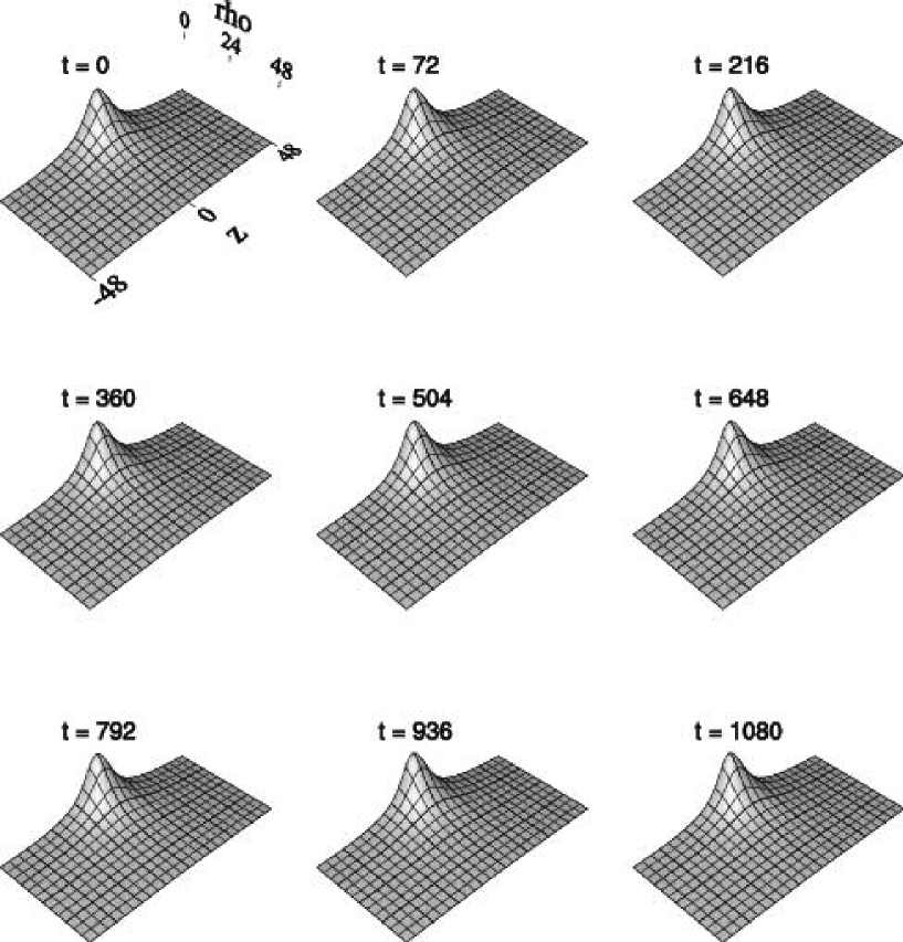
Figure 2: Unigrid static boson star code test: $\psi(t,\rho,z)$. The figure shows $N=128$ calculation. The initial central value of the scalar field is $\phi_{0}(0)=0.02$. As is the case for $|\phi(t,\rho,z)|$ (Fig. 1), $\psi(t,\rho,z)$ is time-independent to eye-ball accuracy. $1.004\leq\psi(t,\rho,z)\leq 1.048$.

F.2 Time-independence of $\max_{\rho,z}|\phi(t,\rho,z)|$

Fig. 3 plots the maximum value of the modulus of the scalar field, $\max_{\rho,z}|\phi(t,\rho,z)|$, vs $t$ from the $N=128$ calculation. The figure shows that the maximum value exhibits periodic oscillations as well as a drift that is due to the accumulation of solution error. We fully expect to see such oscillations since numerical errors act as a perturbation to the “exact” stationary solution. 

It is an instructive exercise to compare the observed period of oscillation with that computed from perturbation analysis of the initial boson star as described in Sec. (0.17.4). Assuming harmonic time-dependence for the perturbed scalar field and metric component (120), (121), and assuming that the oscillation is in the fundamental mode, we obtain a theoretical value of $\sigma^{2}\approx 0.00035$. (Time averaging $\phi_{0}(t,0)$ gives $\langle\phi_{0}(t,0)\rangle\approx 0.02\times\sqrt{4\pi}=0.071$. ) On the other hand, Fig. 3 shows a period of oscillation $T\approx 382$, corresponding to a frequency $\sigma\equiv 2\pi/T=0.0164$. The average of the lapse function is $\langle\alpha(t,0)\rangle=0.993$, therefore $\sigma^{2}/\alpha^{2}\approx 0.00032$, in good agreement with the perturbation analysis value $0.00035$.

Figure 3: Unigrid static boson star code test: Oscillation of $\max_{\rho,z}|\phi(t,\rho,z)|$ as a measure of perturbation. Results shown here are from the $N=128$ calculation. The initial central value of the scalar field is $\phi_{0}(0)=0.02$. The observed oscillation frequency is roughly $\sigma^{2}\approx 0.00032$, and is in good agreement with the fundamental mode frequency computed from perturbation analysis, $\sigma^{2}\approx 0.00035$.

F.3 Time-independence of ADM Mass

Fig. 4 shows the ADM mass $M_{\rm ADM}(t)$ vs time $t$ for the $N=128$ simulation. The general increase in mass starting at $t\approx 450$ is indicative of an instability, and implies that the evolution will generically break down for a sufficiently long evolution.

Figure 4: Unigrid static boson star code test: $M_{\rm ADM}(t)$ for $N=128$ calculation. The initial central value of the scalar field is $\phi_{0}(0)=0.02$. The general increase in mass starting at $t\approx 450$ is indicative of an instability, and implies that the evolution will generically break down for a sufficiently long evolution. In the inset, we show a detail view of the initial fluctuations in $M_{\rm ADM}(t)$.

F.4 Convergence tests of $\max_{\rho,z}(|\phi(t,\rho,z)|)$ and $M_{\rm ADM}(t)$

Figs. 5 shows the maximum value of the modulus of the scalar field, $\max_{\rho,z}(|\phi(t,\rho,z)|)$, vs $t$ from the calculations at the four different finite difference resolutions, $N=64,128,256$ and $512$. Fig. 6 similarly shows the ADM mass as a function of time for the four calculations. The two figures provide strong evidence that both quantities are converging. Finally, Fig. 7 shows the convergence $Q$-factor for ${\rm Re}(\phi(t,\rho,z))\equiv\phi_{1}(t,\rho,z)$, where the $Q$-factor for a general grid function $u^{h}$ is defined by

$$Q\equiv\frac{\|u^{4h}-u^{2h}\|_{2}}{\|u^{2h}-u^{h}\|_{2}}\,,$$ (1)

and which has a theoretical value $Q=4$ for a second order scheme. Here $\|\cdot\|_{2}$ denotes the $l_{2}$ norm, and $h=\Delta\rho=\Delta z$.

Figure 5: Unigrid static boson star code test: 4-level convergence test of $\max_{\rho,z}|\phi(t,\rho,z)|$. The figure shows that $\max_{\rho,z}|\phi(t,\rho,z)|$ converges to a constant as $\Delta\rho,\Delta z\to 0$.

Figure 6: Unigrid static boson star code test: 4-level convergence test of ADM mass $M_{\rm ADM}(t)$. The figure shows that $M_{\rm ADM}(t)$ generally converges to a constant as $\Delta\rho,\Delta z\to 0$, although there are clearly indications of some problems at later times in this plot which are almost certainly a result of imperfect boundary conditions.

Figure 7: Unigrid static boson star code test: Convergence rate of ${\rm Re}(\phi(t,\rho,z))\equiv\phi_{1}(t,\rho,z)$. The theoretical value for a second-order convergent scheme is $Q=4$. See text for further explanation.

References

- [1] S. H. Hawley. Scalar Analogues of Compact Astrophysical Systems. PhD thesis, The University of Texas at Austin, (2000).
- [2] S. H. Hawley and M. W. Choptuik. Boson stars driven to the brink of black hole formation. Phys. Rev., D62:104024, (2000).
- [3] D. J. Kaup. Klein-gordon geon. Phys. Rev., 172:1331, (1968).
- [4] P. Jetzer. Boson stars. Phys. Rep., 220:163, (1992).
- [5] L. Lehner. Numerical relativity: A review. Class. Quantum Grav., 18:R25–R86, (2001).
- [6] M. J. Berger and J. Oliger. Adaptive mesh refinement for hyperbolic partial differential equations. J. Comp. Phys., 53:484, (1984).
- [7] M. W. Choptuik. Universality and scaling in gravitational collapse of a massless scalar field. Phys. Rev. Lett., 70:9, (1993).
- [8] F. Pretorius. Numerical Simulations of Gravitational Collapse. PhD thesis, The University of British Columbia, (2002).
- [9] M. W. Choptuik, E. W. Hirschmann, S. L. Liebling, and F. Pretorius. An axisymmetric gravitational collapse code. Class. Quantum Grav., 20:1857–1878, (2003).
- [10] F. E. Schunck and E. W. Mielke. General relativistic boson stars. Class. Quantum Grav., 20:R301–R356, (2003).
- [11] T.W. Baumgarte and S.L. Shapiro. Numerical relativity and compact binaries. Phys. Rep., 376:41–131, (2003).
- [12] J. A. Wheeler. Geons. Phys. Rev., 97:511, (1955).
- [13] R. Ruffini and S. Bonazzola. Systems of self gravitating particles in general relativity and the concept of an equation of state. Phys. Rev., 187:1767, (1969).
- [14] B. K. Harrison, K. S. Thorne M. Wakano, and J. A. Wheeler. Gravitation Theory and Gravitational Collapse. University of Chicago Press, Chicago, (1965).
- [15] S. Weinberg. Gravitation and Cosmology : Principles and Applications of the General Theory of Relativity. Wiley, (1972).
- [16] T. D. Lee and Y. Pang. Stability of mini-boson stars. Nucl. Phys., B315:477, (1989).
- [17] M. Gleiser and R. Watkins. Gravitational stability of scalar matter. Nucl. Phys., B319:733, (1989).
- [18] E. Seidel and W. M. Suen. Dynamical evolution of boson stars: Perturbing the ground state. Phys. Rev., D42:384–403, (1990).
- [19] J. Balakrishna and W. M. Suen. Dynamical evolution of boson stars. II. excited states and self-interacting fields. Phys. Rev., D58:104004, (1998).
- [20] S. L. Shapiro and S. A. Teukolsky. Black Holes, White Dwarfs, and Neutron Stars. Wiley, (1983).
- [21] Y. Kobayashi, M. Kasai, and T. Futamase. Does a boson star rotate? Phys. Rev., D50:7721, (1994).
- [22] J. B. Hartle. Slowly rotating relativistic stars. I. equations of structure. Astrophys. J., 150:1005, (1967).
- [23] J. B. Hartle and K. S. Thorne. Slowly rotating relativistic stars. II. models for neutron stars and supermassive stars. Astrophys. J., 153:807, (1968).
- [24] V. Silveira and C. M. G. de Sousa. Boson star rotation: A Newtonian approximation. Phys. Rev., D52:5724, (1995).
- [25] R. Ferrell and M. Gleiser. Gravitational atoms: Gravitational radiation from excited boson stars. Phys. Rev., D40:2524, (1989).
- [26] F. E. Schunck and E. W. Mielke. Rotating boson stars. In F. W. Hehl, R. A. Puntigam, and H. Ruder, editors, Relativity and Scientific Computing, pages pp. 138–151, Berlin, (1996). Springer.
- [27] S. Yoshida and Y. Eriguchi. Rotating boson stars in general relativity. Phys. Rev., D56:762–771, (1997).
- [28] S. Yoshida and Y. Eriguchi. New static axisymmetric and nonvacuum solutions in general relativity: equilibrium solutions of boson stars. Phys. Rev., D55:1994, (1997).
- [29] C. Gundlach. Critical phenomena in gravitational collapse. Phys. Rep., 376:339–405, (2003).
- [30] S. Noble. A Numerical Study of Relativistic Fluid Collapse. PhD thesis, The University of Texas at Austin, (2003).
- [31] B. Rousseau. Axisymmetric boson stars in the conformally flat approximation. Master’s thesis, The University of British Columbia, (2003).
- [32] D. Choi. Numerical Studies of Nonlinear Schrödinger and Klein-Gordon Systems: Techniques and Applications. PhD thesis, The University of Texas at Austin, (1998).
- [33] S. W. Hawking and G. F. R. Ellis. The Large Scale Structure of Space-Time. Cambridge University Press, Cambridge, (1973).
- [34] C. M. Will. Theory and Experiment in Gravitational Physics. Cambridge University Press, revised edition, (1993).
- [35] C. M. Will. The confrontation between general relativity and experiment. Living Reviews in Relativity, http://relativity.livingreviews.org/Articles/lrr-2001-4, (2001).
- [36] C. M. Will. The confrontation between general relativity and experiment. Astrophysics and Space Science, 283:543–552, (2003).
- [37] R. Arnowitt, S. Deser, and C. W. Misner. In L. Witten, editor, Gravitation: An Introduction to Current Research. New York, Wiley, (1962).
- [38] J. W. York, Jr. In L. Smarr, editor, Sources of Gravitational Radiation. Seattle, Cambridge University Press, (1979).
- [39] K. Maeda, M. Sasaki, T. Nakamura, and S. Miyama. A new formalism of the Einstein equations for relativistic rotating systems. Prog. Theor. Phys., 63:719, (1980).
- [40] R. Geroch. A method for generating solutions of Einstein’s equations. Jour. Math. Phys., Vol.12(No. 6):918, (1971).
- [41] S. L. Liebling. Nonlinear Field Dynamics in General Relativity: Black Hole Critical Phenomena and Topological Defects. PhD thesis, The University of Texas at Austin, (1998).
- [42] J. D. Anderson, Jr. Computational Fluid Dynamics: The Basics with Applications. McGraw-Hill, (1995).
- [43] H. Kreiss and J. Oliger. Methods for the approximate solution of time dependent problems. Global Atmospheric Research Programme, Publications Series No. 10, (1973).
- [44] M. W. Choptuik. A study of numerical techniques for the initial value problem of general relativity. Master’s thesis, The University of British Columbia, (1982).
- [45] W. H. Press et al. Numerical recipes in FORTRAN : the art of scientific computing. Cambridge University Press, (1992).
- [46] W. Hackbusch and U. Trottenberg. In W. Hackbusch and U. Trottenberg, editors, Multigrid methods : proceedings of the conference held at Köln-Porz, November 23-27, 1981. Berlin: Springer-Verlag, (1982).
- [47] A. Brandt. Multi-level adaptive solutions to boundary-value problems. Math. Comput., 31:333, (1977).
- [48] C. W. Ueberhuber. Numerical Computation 2: Methods, Software, and Analysis. Springer-Verlag, (1997).
- [49] E. Schnetter, S. H. Hawley, and I. Hawke. Evolutions in 3D numerical relativity using fixed mesh refinement. Class. Quantum Grav., 21:1465–1488, (2004).
- [50] B. Brügmann, W. Tichy, and N. Jansen. Numerical simulation of orbiting black holes. Phys. Rev. Lett., 92:211101, (2004).
- [51] M. W. Choptuik, E. W. Hirschmann, S. L. Liebling, and F. Pretorius. Critical collapse of the massless scalar field in axisymmetry. Phys. Rev., D68:044007, (2003).
- [52] M. W. Choptuik, E. W. Hirschmann, S. L. Liebling, and F. Pretorius. Critical collapse of a complex scalar field with angular momentum. gr-qc/0405101, (2004).
- [53] J. Thornburg. Coordinates and boundary conditions for the general relativistic initial data problem. Class. Quantum Grav., 4:1119, (1987).
- [54] E. Seidel and W. M. Suen. Towards a singularity-proof scheme in numerical relativity. Phys. Rev. Lett., 69:1845, (1992).
- [55] M. Alcubierre and B. Brügmann. Simple excision of a black hole in 3+1 numerical relativity. Phys. Rev., D63:104006, (2001).
- [56] H. Yo, T.W. Baumgarte, and S.L. Shapiro. Numerical testbed for singularity excision in moving black hole spacetimes. Phys. Rev., D64:124011, (2001).
- [57] M. Alcubierre et al. Black hole excision for dynamic black holes. Phys. Rev., D64:061501, (2001).
- [58] M.A Scheel et al. Toward stable 3D numerical evolutions of black-hole spacetimes. Phys. Rev., D66:124005, (2002).
- [59] H. Yo, T.W. Baumgarte, and S.L. Shapiro. Improved numerical stability of stationary black hole evolution calculations. Phys. Rev., D66:084026, (2002).
- [60] G. Calabrese et al. Novel finite-differencing techniques for numerical relativity: application to black-hole excision. Class. Quantum Grav., 20:L245–L251, (2003).
- [61] T.W. Baumgarte and S.L. Shapiro. Collapse of a magnetized star to a black hole. Astrophys. J., 585:930–947, (2003).
- [62] D. Shoemaker et al. Moving black holes via singularity excision. Class. Quantum Grav., 20:3729, (2003).
- [63] G. Calabrese and D. Neilsen. Spherical excision for moving black holes and summation by parts for axisymmetric systems. Phys. Rev., D69:044020, (2004).
- [64] S. H. Hawley. Private Communication (2003).
- [65] S. M. Carroll. Lecture notes on general relativity. gr-qc/9712019, (1997). Eq. (7.5).
- [66] M. W. Choptuik. A Study of Numerical Techniques for Radiative Problems in General Relativity. PhD thesis, The University of British Columbia, (1986).
- [67] C. W. Misner, K. S. Thorne, and J. A. Wheeler. Gravitation. W.H. Freeman and Company, New York, (1973).
- [68] L.I. Petrich, S.L. Shapiro, and S.A. Teukolsky. Oppenheimer-Snyder collapse with maximal time slicing and isotropic coordinates. Phys. Rev., D31:2459, (1985).
- [69] M.W. Choptuik. Consistency of finite-difference solutions of Einstein’s equations. Phys. Rev., D44:3124, (1991).
- [70] Evans C. R. A method for numerical relativity: Simulation of axisymmetric gravitational collapse and gravitational radiation generation. PhD thesis, The University of Texas at Austin, (1984).
- [71] R. Friedberg, T.D. Lee, and Y. Pang. Mini-soliton stars. Phys. Rev., D35:3640–57, (1987).
- [72] J. Ventrella. A Numerical Treatment of Spin- Fields Coupled to Gravity. PhD thesis, The University of Texas at Austin, (2002).
- [73] R. D’Inverno. Introducing Einstein’s Relativity. Oxford University Press, New York, (1992).
- [74] A. P. Lightman et al. Problem Book in Relativity and Gravitation. Princeton University Press, (1975). Problem 15.3.
- [75] D. Choi. http://lheawww.gsfc.nasa.gov/~choi/axi/axi.html.
- [76] J.L. Friedman, J.R. Ipser, and L. Parker. Models of rapidly rotating neutron stars. Nature, 312:255, (1984).
- [77] M.A. Ruderman and P.G. Sutherland. Rotating superfluid in neutron stars. Astrophys. J., 190:137–9, (1974).
- [78] B.J. Owen et al. Gravitational waves from hot young rapidly rotating neutron stars. Phys. Rev., D58:084020, (1998).
- [79] S.I. Yoshida, S. Karino, S. Yoshida, and Y. Eriguchi. A numerical study of the r-mode instability of rapidly rotating nascent neutron stars. MNRAS, 316:L1–4, (2000).
- [80] T.E. Strohmayer. Gravitational waves from rotating neutron stars and evaluation of fast chirp transform techniques. Class. Quantum Grav., 19:1321–1326, (2002).
- [81] F.E. Schunck and E.W. Mielke. Rotating boson star as an effective mass torus in general relativity. Phys. Lett. A, 249:389–94, (1998).
- [82] S. Chandrasekhar. The Mathematical Theory of Black Holes. Oxford University Press, (1983).
- [83] L. Komzsik. Implicit computational solution of generalized quadratic eigenvalue problems. Finite Elements in Analysis and Design, 37(10):799–810, (2001).
- [84] S.R. Kohn and S.B. Baden. The parallelization of an adaptive multigrid eigenvalue solver with LPARX. In Proceedings of the Seventh SIAM Conference on Parallel Processing for Scientific Computing, page 552, (1995).
- [85] S. Costiner and S. Ta’asan. Adaptive multigrid techniques for large-scale eigenvalue problems: Solutions of the Schrödinger problem in two and three dimensions. Phys. Rev., E51:3704–3717, (1995).
- [86] R. Burden and J. Faires. Numerical Analysis. Brooks-Cole Publishing, 7th edition, (2001). pp.635.
- [87] R. Guenther. A Numerical Study of The Time Dependent Schödinger Equation Coupled with Newtonian Gravity. PhD thesis, The University of Texas at Austin, (1995).
- [88] R. C. Tolman. On the use of the energy-momentum principle in general relativity. Phys. Rev., 35:875, (1930).
- [89] R. M. Wald. General Relativity. University of Chicago Press, Chicago IL, (1984).
- [90] A. Ashtekar and A. Magnon-Ashtekar. On conserved quantities in general relativity. J. Math. Phys., 20:793–800, (1979).
- [91] M. Choptuik. Private Communication (2004).
- [92] F. D. Ryan. Spinning boson stars with large self-interaction. Phys. Rev., D55:6081–6091, (1997).
- [93] M. Colpi, S. L. Shapiro, and I. Wasserman. Boson stars: Gravitational equilibria of self-interacting scalar fields. Phys. Rev. Lett., 57:2485–2488, (1986).
- [94] http://www.netlib.org/eispack.
- [95] B. F. Schutz. A First Course in General Relativity. Cambridge University Press, (1985). pp.200.
- [96] F. Pretorius, Unpublished work, (2004).