THE CAMPBELL–MAGAARD THEOREM IS INADEQUATE

AND INAPPROPRIATE AS A PROTECTIVE THEOREM

FOR RELATIVISTIC FIELD EQUATIONS

Edward Anderson^∗

Astronomy Unit, School of Mathematical Sciences, Queen Mary, University of London, UK

Given a particular prescription for the Einstein field equations, it is important to have general protective theorems that lend support to it. The prescription of data on a timelike hypersurface for the ($n$ + 1)-d Einstein field equations arises in ‘noncompact Kaluza–Klein theory’, and in certain kinds of braneworlds and low-energy string theory. The Campbell–Magaard theorem, which asserts local existence (and, with extra conditions, uniqueness) of analytic embeddings of completely general $n$-d manifolds into vacuum ($n$ + 1)-d manifolds, has often recently been invoked as a protective theorem for such prescriptions.

But in this paper I argue that there are problems with loosening the Campbell–Magaard theorem of restricitive meanings in its statement, which is a worthwhile thing to do in pursuit of the proposed applications. While I remedy some problems by identifying the required topology, delineating what ‘local’ can be taken to mean, and offering a new, more robust and covariant proof, other problems with the proposed applications remain insurmountable. The theorem lends only inadequate support, both because it offers no guarantee of continuous dependence on the data and because it disregards causality. Furthermore, the theorem is only for the analytic functions which renders it inappropriate for the study of the relativistic field equations of modern physics.

Unfortunately, there are as yet no known general theorems that offer adequate protection to the proposed applications’ prescription. I conclude by making some suggestions for more modest progress.

^∗ Next addresses: as of Oct 2004, Peterhouse College Cambridge UK and DAMTP Cambridge UK;

additionally, as of Jan 2005, Department of Physics, P-412 Avadh Bhatia Physics Laboratory, University of Alberta, Edmonton, Alberta, Canada.

Email addresses: eda@maths.qmul.ac.uk, ea212@cam.ac.uk

1 Introduction

The Campbell–Magaard (CM) theorem [2, 3] concerns the existence (and with extra conditions uniqueness) of embeddings of $n$-d manifolds into vacuum ($n$ + 1)-d manifolds. This theorem, qualified as ‘old and little known’, has recently been claimed to lend support [4, 5, 6, 7, 9, 10, 11] to ‘space-time-matter’ or ‘noncompactified Kaluza–Klein’ (NKK) theory [5, 12, 13, 14]. This is a proposed 5-d toy model for the investigation of the consequences of higher-d physics. In this article, I question the suitability of the CM theorem for such an application and hence I question the foundations of NKK theory. Reasons to consider NKK seriously enough to ask such questions include 1) that one may be able to untangle and then understand some of the many effects of higher-d physics by such models, and 2) that NKK theory is playing a role in experimental predictions and proposals [15, 7]; it even plays a role in a recent cover feature in the New Scientist [8].

Further reasons to question the applicability of the CM theorem are that it has also appeared in connection with constructing higher-d GR solutions [16, 17], low-energy string theory solutions [18] and lower-d gravity [17]. The CM theorem generalizes [9, 19, 20] to a wider range of situations in higher-d physics, where cosmological constants and scalar fields are commonplace. The CM theorem and its generalizations have also been suggested [21, 22] as an underlying theorem relevant for building certain types of braneworlds (see also [26]), and have also been studied in various other contexts, e.g [27, 28, 29, 30, 10, 11].

In this paper, serious difficulties with using the CM theorem for these applications are revealed and studied. It is in the interest of the proposed applications to have protective results in extended regions. Moreover, the historical development of the GR Cauchy and initial-value problems (Sec 2–4) provides both guidance and limitations on this pursuit. I argue (Secs 2–4) that the CM theorem can be seen as a collection of workings each of which is of a well-known type from the roughly contemporary (very early) GR CP and IVP literature. This was not picked up by Magaard [3], by the historians [31, 32, 33] or in the introduction of the theorem into the modern literature [4]. I consider limitations on the extendibility of Magaard’s proof of the CM theorem toward a proof that would be of greater value for the proposed applications in Secs 4–7. I provide improvements on Magaard’s proof in Secs 5-6, which include identifying the required topology, spelling out what the word ‘local’ can and cannot be taken to mean in the statement of the theorem, and working covariantly. However, other problems with such a program remain insurmountable (Sec 7). The theorem offers only inadequate support both because it can not encompass continuous dependence on the data and because it disregards causality. Furthermore, the theorem is solely about the analytic functions which renders it inappropriate for the study of the relativistic field equations of modern physics. Thus there are strong reasons why the CM theorem should not be taken seriously as a protective theorem for general relativistic field equations.

I conclude in Sec 8.1 with the case against the CM theorem, and in Sec 8.2 with an account of how in the case of its applications proposed in the literature there is currently no other satisfactory general protective theorem known. Thus these proposed applications remain unprotected. In Sec 8.3 I discuss the position of NKK theory in this light. In Sec 8.4 I point out that the construction of particular examples in various claimed applications do not actually make contact with the CM theorem. The methods actually used in these examples are often rather among the cruder simplifications of the well-known Lichnerowicz–York conformal method for the IVP [48, 49, 41, 50]. Finally in Sec 8.5 I discuss some more limited ways to approach the braneworld application while staying within bona fide mathematical physics.

2 Campbell and his contemporaries

Campbell, while primarily a pure mathematician, was well aware of GR [51]. However, his 1926 book presents what is a split of the ($n$ + 1)-d Euclidean version of the vacuum Einstein field equations (EFE’s) ${\cal R}_{AB}=0$ with respect to a $n$-d hypersurface $\mu=const$ without any comments about, or applications to, GR. The split is

$$0={\cal R}_{ab}=R_{ab}+\epsilon\left(\Omega_{ab}\Omega-2{\Omega_{a}}^{c}\Omega_{bc}\right)-\frac{\epsilon}{\phi}\frac{\partial\Omega_{ab}}{\partial\mu}\quad+\frac{1}{\phi}D_{a}D_{b}\phi\mbox{ },$$ (1)

$$0={\cal R}_{a\mu}=\frac{\epsilon}{\phi}\left(D^{b}\Omega_{ab}-D_{a}\Omega\right)\mbox{ },$$ (2)

$$0={\cal R}_{\mu\mu}=\frac{\partial\Omega}{\partial\mu}-\epsilon\phi D^{2}\phi-\Omega_{ab}\Omega^{ab}\mbox{ }.$$ (3)

$$\mbox{Here, }\mbox{\hskip 36.135pt}g_{AB}=\left(\begin{array}[]{ll}h_{ab}&0\\ 0&\epsilon\phi^{2}\\ \end{array}\right)\mbox{\hskip 36.135pt},\mbox{\hskip 36.135pt}\epsilon=1\mbox{\hskip 36.135pt}\mbox{and}\mbox{\hskip 36.135pt}\Omega_{ab}=-\frac{1}{2\phi}\frac{\partial h_{ab}}{\partial\mu}\mbox{ }.\mbox{\hskip 36.135pt}$$

He eventually identified $n+1$ of these equations, (2) and $\left[(\ref{mumu})-\frac{1}{2}\mbox{ trace}(\ref{ab})\right]$ i.e

$$R-\Omega_{ab}\Omega^{ab}+\Omega^{2}=0\mbox{ },$$ (4)

as being ‘different’ from the other equations (1). So there are two systems to treat separately. He then proposed, but by no means proved, the following conjecture about the above split.

Campbell’s conjecture Any $n$-space is ‘surrounded’ by a vacuum ($n$ + 1)-space.

What he offered as a piece of a proof for this is that the ‘different’ equations (2, 4) propagate away from the original $\mu=const$ hypersurface.

It is however illuminating to consider Campbell’s work within its proper historical context. He appears to have been unaware that his relativist contemporaries were in the middle of learning about the conceptualizations of such splits. In any case, Campbell’s book and death pre-date the consolidation of these conceptualizations in Darmois’ 1927 article [35]. Because Darmois’ work was substantial and has been built on a great deal (this is the famous French school’s contribution to mathematical relativity [48, 53, 36, 37]… ), the timing of the appearance of Campbell’s above work about the split is unfortunate. Campbell’s account indeed lacks this very useful conceptual understanding (which has subsequently become common knowledge both via the French school’s work and the foundations of canonical GR [54]).

Here is the conceptualization and how it was gradually being discovered by Campbell’s contemporaries. At the simplest level, altering the ($n$ + 1)- or $n$-d signature in the split (so as to seek GR applications) is immaterial. [I smuggled this into the above presentation (1–3) of the split by bringing in an $\epsilon$ which can be set to $-1$ in the case where the $\mu$-direction is timelike; the hypersurface’s signature does not feature explicitly in (1–3)]. There are two notable GR applications. First, the split of the Lorentzian vacuum EFE’s with respect to an entirely spatial hypersurface ($\mu=t$, a time function) is important because of its dynamical significance. Second, the split of the Lorentzian vacuum EFE’s with respect to a timelike hypersurface can be applied to obtaining junction conditions. This plays no role in this paper until Sec 8.

There are also some inter-related geometrical interpretations. G1: $\Omega_{ab}$ is none other than the extrinsic curvature $K_{ab}$. G2: the ‘different’ equations, or constraints (2,4), are contractions of the well-known Gauss and Codazzi embedding conditions [55]. G3: one is better served by splitting from the outset the Einstein tensor ${\cal G}_{AB}\equiv{\cal R}_{AB}-\frac{{\cal R}}{2}g_{AB}=0$ and not the Ricci tensor ${\cal R}_{AB}=0$ whereupon the constraints (2, 4) arise automatically as ${\cal G}_{A\mu}=0$. G4: there are ‘relations’ between the quantities in the EFE’s. G5: These ‘relations’ are none other than the contracted Bianchi identity

$$0=\nabla_{B}{{\cal G}_{A}}^{B}=\partial_{\mu}{\cal G}_{A}{}^{\mu}+\partial_{i}{{\cal G}_{A}}{}^{i}-{{\cal G}_{A}}{}^{B}{{\Gamma}^{\mu}}{}_{B\mu}+{{\cal G}_{B}}{}^{\mu}{{\Gamma}^{B}}{}_{A\mu}\mbox{ }.$$ (5)

The form in G3 of the constraints makes it immediately obvious that the propagation of the constraints is automatically guaranteed, so there is no need to check longhand for this. (As regards his conjecture, Campbell’s ‘partial proof’ consisted just of establishing this propagation longhand, therefore he proved nothing at all.)

Finally, the inclusion of a wide range of matter types does not upset the above conceptualizations. One then splits up the full EFE’s ${\cal G}_{AB}={\cal T}_{AB}$ rather than the vacuum ones.

Hilbert in 1917 [56] was the first to recognize that the EFE’s contain two systems to be treated separately. He had some idea of the dynamical application and was aware of G4 but not G5. Levi-Civita pointed out G5 later in 1917 [57]. In their 1923 textbook, Birkhoff and Langer [58] stated the dynamical application and explained G4–G5, although they did not explicitly provide the split equations. Also in 1923, Lanczos [59] conceived of the junction application. Darmois collected or discovered all of the above conceptualizations in his 1923–1927 program [34, 35]. Hilbert and Darmois considered between them a wide range of matter in addition to the vacuum case.

3 Early development of the GR initial value and Cauchy problems

I now consider the early development of the study of the two separate systems found above within the EFE’s: the GR IVP [solving (2), (4)] and the GR CP [solving (1)]. My account picks out material important for the discussion of Magaard’s development of Campbell’s conjecture in the next section.

To prove statements like Campbell’s conjecture, what one requires is what Darmois [35] pointed out: for contact to be established between the constraint and evolution subsystems of the EFE’s and the formal theory of p.d.e’s. Now, the Cauchy–Kowalewskaya (CK) theorem [60] could be applied here; after all, it can be applied to almost any type of p.d.e system.

Cauchy–Kowalewskaya theorem: suppose one has A unknowns $\Psi_{\mbox{\scriptsize A\normalsize}}$ which are functions of an independent dynamical variable $\mu$ and of Z other independent variables $x_{\mbox{\scriptsize Z\normalsize}}$. Suppose one is prescribed on some domain $\Omega$ the A p.d.e’s of order $k$ of form $\frac{\partial^{(k)}\Psi_{\mbox{\tiny A\normalsize}}}{\partial\mu^{(k)}}=F_{\mbox{\scriptsize A\normalsize}}$ where the $F_{\mbox{\scriptsize A\normalsize}}$ are functions of $\mu$, $x_{\mbox{\scriptsize Z\normalsize}}$, $\Psi_{\mbox{\scriptsize A\normalsize}}$ and of derivatives of $\Psi_{\mbox{\scriptsize A\normalsize}}$ up to ($k$ – 1)th order w.r.t $\mu$; furthermore suppose that in $\Omega$ the $F_{\mbox{\scriptsize A\normalsize}}$ are analytic functions of their arguments. Suppose one is further prescribed analytic data $\Psi_{\mbox{\scriptsize A\normalsize}}(0,x_{\mbox{\scriptsize Z\normalsize}})={}^{(0)}d_{\mbox{\scriptsize A\normalsize}}(x_{\mbox{\scriptsize Z\normalsize}})$, … , $\frac{\partial^{(k-1)}\Psi_{\mbox{\tiny A\normalsize}}}{\partial\mu^{(k-1)}}(0,x_{\mbox{\scriptsize Z\normalsize}})={}^{(k-1)}d_{\mbox{\scriptsize A\normalsize}}(x_{\mbox{\scriptsize Z\normalsize}})$ on some nowhere-characteristic piece $W$ of the boundary of $\Omega$. Then there locally exists a unique analytic solution.

N.B the casting of the evolution equations into CK form is robust as regards to what choice is made for the $n$- and ($n$ + 1)-d signature, so theorems based on the CK theorem would appear to have a wide range of different GR applications.

What is delicate however is the requirement of analyticity. Now, Darmois was well aware of the arguments (e.g in Hadamard’s 1923 book [61]) against the CK theorem and the use of analytic functions. The analytic functions are very special in the sense that theorems holding for these may well not hold on other sorts of function spaces. Moreover, sole consideration of the analytic functions is inappropriate for the study of ‘causal’ or ‘relativistic’ field equations because they are rigid: one cannot prescribe data independently in causally-disconnected regions as one would desire for physical modeling because the one data patch admits a unique and obligatory analytic continuation into the other data patch. Furthermore, as Hadamard points out, the fact that other functions can be arbitrarily-approximated by analytic functions is not per se an adequate counter-argument to this. It would only become relevant in p.d.e problems for which the continuous dependence of the solution on the data can be established. This is in itself an important physical requirement, for we never know data exactly, so we would have no physical predictivity unless it is guaranteed that tiny undetectable changes in the data do not immediately and grossly alter the behaviour of the solution. In order to have a sensible p.d.e problem in mathematical physics, it should be well-posed, which requires continuous dependence (and yet further conditions for certain types of p.d.e) in addition to existence and uniqueness. Now, notably, the CK theorem is inadequate for establishing these important additional properties [61, 62, 42]. Theorems about particular p.d.e systems that are based on the analytic functions alone constitute inadequate mathematical physics. In the context of relativistic field equations, they also constitute inappropriate mathematical physics. Thus such theorems should not be taken very seriously in this context.

Thus I see it as significant that while Darmois was well aware of the possibility of applying the CK theorem, he did not advocate any such proof for the Einstein evolution equations in his 1927 article. While e.g Cartan did put forward a proof of this kind in 1931 [63], note that this work does not mention analyticity nor physics but rather that it takes on trust that the reader is aware of the CK theorem (and presumably this includes the above awareness of limitations so that this work should be viewed as a purely mathematical exercise). Stellmacher in 1938 [64] was the first to successfully abandon the analytic functions so as to bring out the causal nature of spacetime. The significance of abandoning the analytic functions was repeatedly stressed, e.g in Lichnerowicz’s [48] and Fourès-Bruhat’s [36] foundational papers on the GR IVP and CP and on p 440 of Courant and Hilbert [62].

It should be noted that these advances are most very specific about the signatures involved i.e about the $n$-d hypersurface being spacelike and the extra dimension being timelike. Thus for the GR CP, inadequate and inappropriate analytic function results can be replaced by respectable theorems, but whether this is the case for any analogous problems with different signature is unknown (see Sec 7). As Hilbert pointed out in 1917 [56], the GR CP’s advances proceed via breaking manifest general covariance by coordinate fixings (nowadays called gauge choices [65]) that are special in that the evolution equations are then cast as a hyperbolic system. While the evolution equations (1) are presented above in a form close to normal gauge (which would additionally have $\phi$ = 1), it is rather the harmonic gauge developed by DeDonder and by Lanczos in 1921-1923 [66, 67] (see also Darmois 1927) that is used to establish a hyperbolic system.

The GR IVP began with Lichnerowicz 1944 [48]. He discards the normal coordinates (which are mathematically unfortunate because they are prone to focusing leading to their breakdown by caustic formation $K\longrightarrow 0$) in favour of the quite deliberately defocussing maximal gauge $K=0$. He then considers the lower-dimensional metric to be known up to a conformal factor which is then to be determined by solving the conformally-transformed Gauss constraint. This started the conformal method for the GR IVP later substantially developed by York [49, 41]; this underlies much of today’s compact-binary numerical relativity [68, 45, 46].

It is furthermore relevant that Lichnerowicz’s work does not yet include global considerations. I.e whether proposed results are local or global, and whether then they depend on the type of $n$-space e.g whether it is compact without boundary or asymptotically flat. As an example of global unawareness, it so happens that the maximal gauge cannot be maintained if one wishes to work globally with compact without boundary $n$-spaces; this was only later remedied by York’s development of the constant mean curvature gauge ($K=C$, a spatial constant) [49].

4 Fourès-Bruhat’s criticisms versus Magaard’s argument

Another significant early article for the GR IVP is Fourès Bruhat 1956 [37]. This includes arguments for the conformal approach, favouring it over the following ‘componentwise algebraic elimination method’. Suppose a diagonal extrinsic curvature component (without loss of generality $K_{11}$) is available among the quantities to be regarded as unknowns. Then one can choose to interpret the Gauss constraint as a linear equation for this, as is made manifest by writing the Gauss constraint in terms of the manifestly antisymmetric inverse DeWitt [69] supermetric $G^{ijkl}=h^{ik}h^{jl}-h^{ij}h^{kl}$:

$$2K_{11}G^{11uw}K_{uw}+G^{1u1w}K_{1u}K_{1w}+G^{uwxy}K_{uw}K_{xy}=-\epsilon R\mbox{ },$$ (7)

where $u$, $w$, $x$, $y$ $\neq 1$. Thus, provided that $Z\equiv G^{11uw}K_{uw}$ has no zeros in the region of interest, $K_{11}$ can be straightforwardly eliminated in the Codazzi constraint, which one may then attempt to treat as a p.d.e system for the other unknowns.

Fourès-Bruhat’s first criticism of the above is that this restriction due to the possibility of zeros of $Z$ is undesirable. Moreover, this particular ‘Problem of Zeros’ is a severe restriction because, firstly, it invalidates the eliminated system itself, undermining from the start any p.d.e theorems about this system. Secondly, since $Z$ is a function of all the metric components and of all bar $n+1$ of the extrinsic curvature components, it is a function of at least one unknown so that the occurrence of such zeros within a given region is not known from the outset but rather only once the system is solved!

Fourès-Bruhat’s second criticism of the above is that it is a non-covariant procedure. This contributes to it being highly ambiguous, since the nature of the prescription depends on the choice of coordinates, and there is no unique clear-cut way of choosing which components are to be regarded as the knowns and unknowns.

Magaard was a differential geometry student who was not motivated by GR and was unaware of Bruhat’s work. He proved [3] Campbell’s conjecture upon choosing analyticity and ‘locality’ to be included in the statement: the Campbell–Magaard (CM) theorem. Of course, this is fine as regards differential geometry. However, as argued above, the analyticity means that it is inappropriate to then apply this theorem as an underlying theorem for the study of relativistic field equations. The analyticity is also the key reason why the theorem persists when one alters the signatures from Magaard’s original Riemannian case to the semi-Riemannian case of the proposed applications. I also argued above that proving existence and uniqueness alone, while useful, is inadequate for mathematical physics. Magaard’s use of ‘locality’ would appear necessary to have a theorem at all. Moreover, how far ‘local’ can be extended is a complicated issue not covered by Magaard. But it would favour the proposed applications if a stronger meaning than the neighbourhood of analysis could be attributed to the word ‘local’, as the proposed applications really concern astrophysics and cosmology and quite extended regions of spacetime are required to be included for these to make good sense. Moreover, Magaard approaches the data construction part of the proof by a particular case of the above componentwise algebraic method. And yet he avoids the original impact of the above ‘Problem of Zeros’ by the following sort of argument, although I will show later on that one then has to pay one or two large prices (depending on the signature) if one chooses this method and attempts to consider more extended regions.

Magaard’s argument: one is entitled to declare that some $(n-1)$-d set $X=\{x_{1}=\mbox{ some const}\}$ is to play the role of a (partial) boundary in the construction of data on an adjacent $n$-d set $W$. Then, one is entitled to prescribe ‘data for the data’ on this boundary set, i.e the values that the knowns take there and a free choice of boundary values for the unknowns too. Thus, although $Z$ is a function of knowns and unknowns in the region of interest away from the boundary set $X$, it is a function of knowns alone on $X$, and these knowns can be prescribed there so that $Z$ is bounded away from zero on $X$. Then by continuity, there are no zeros of $Z$ near $X$.

Because Magaard’s aim is to prove an embedding theorem, his particular method treats the lower-d metric components as knowns. After Magaard’s elimination of $K_{11}$ by use of the Gauss constraint, he next treats the Codazzi constraint as a p.d.e system for the unknowns $K_{1u}$ and some other $K_{vw}$ component denoted $E$. It is for each such choice of extrinsic curvature components that one has uniqueness. This, and the existence, follows from the above satisfying the criteria for the CK theorem if one treats $K_{1u}$ and $E$ as known functions on $X$ and all the other components of $K_{ij}$ bar $K_{11}$ as known functions on $W$ and provided that all of the p.d.es’ coefficients, the knowns and the ‘data for the data’ are analytic. So a unique solution exists.

Magaard then groups [3, 20] this data method and the usual CK local existence of a unique ‘evolution’ to form the (signature-independent) CM theorem. (One can proceed likewise if a cosmological constant or a large range of matter fields are included: the generalized Campbell–Magaard theorem [9, 19, 20]).

As regards investigating whether Campbell–Magaard can hold for extended regions, the first price to pay is that although the ‘data for the data’ (values of $K_{1w}$ and $E$ on $X$) can be validly picked so that $Z\neq 0$ on $X$, the protecting continuity argument is only guaranteed to produce a thin strip $W=\{0\leq x_{1}<\eta\}$ before zeros of $Z$ develop.

And one cannot expect to be able to patch these strips together to make data on extended regions (‘Non-patching Problem’). This is because the reason for terminating the construction of the first strip at $x_{1}=\eta$ is that $Z$ is on the verge of picking up zeros. So, while one can construct a second strip that extends beyond these zeros by choosing ‘data for the data’ on {$x_{1}=\eta$} that ensures that $Z$ is bounded away from zero there, clearly then this data does not match up with the first strip’s data across $x_{1}=\eta$. So what one produces is a collection of strips which generally each belong to different possible global data sets. The evolution of each of these strips would then generally produce pieces of different higher-d manifolds.

It is worth making clear that the (generalized) CM theorem should not be used to claim that a vacuum ($n$ + 1)-d manifold ‘surrounds’ any $n$-d manifold. All one can say is that any $n$-d manifold can be cut up in an infinite number of ways (choices of the $x_{1}$ coordinate) into many pieces (the different data patches), each of which can be separately bent in an infinite number of ways (corresponding to the freedom in choosing both the known components of $K_{ij}$ throughout the relevant portion of each $W$ and the unknown components of $K_{ab}$ on each $X$), and for each of these bent regions one can locally find a surrounding ($n$ + 1)-d manifold e.g for every possible analytic function form of ${\cal T}_{AB}$. Given that these embeddings are so nonunique, how can one possibly justify attaching any physical significance whatsoever to any particular example of embedding? The applications suggested in the literature would not seem to be very predictive [20] as their predictions will generally vary depending on the choice of embedding higher-dimensional world. usually give different predictions. N.B this sort of difficulty is by no means confined to embedding scenarios with their large extra dimensions, for conceptually similar difficulties occur in compact extra dimension scenarios (e.g the proliferation of Calabi–Yau spaces [70] in string theory, each of which then gives rise to its own characteristic particle physics). Of course, one may hope to have one day theoretically-motivated selection criteria to overturn this sort of difficulty.

Finally, Fourès-Bruhat’s second criticism still holds since Magaard’s method lacks any $n$-d general covariance as it involves the choice of a coordinate $x_{1}$ and the elimination of a ${11}$-component of a tensor.

5 Building more proofs: other algebraic elimination methods

I first address Fourès-Bruhat’s criticisms by considering two alternatives to Magaard’s proof which I build by using distinct algebraic elimination methods.

The ‘Problem of Zeros’ and subsequent restrictions on region size and the ‘Non-patching Problem’ are badly convoluted for the Magaard method since the zeros of $Z$ are not known until one has solved the complicated eliminated p.d.e system. This obstructs the further study and application of the Magaard method. I proceed otherwise below. Because the application is the proof of an embedding theorem, in this paper I respect the restriction to elimination methods for which the metric is a known (see [71] for a full consideration of 3-d componentwise elimination methods). Consequently the Gauss constraint is to be viewed as an equation for some extrinsic curvature unknown, and is moreover clearly an algebraic equation in this.

5.1 A second componentwise elimination proof

First, I choose this unknown to be a nondiagonal component, which I designate $K_{12}$ without loss of generality. Such a choice is always possible since the constraints require $n+1$ unknowns to be properly determined, and the extrinsic curvature has only $n$ diagonal components. In this case, the Gauss constraint is a quadratic equation:

$$G^{1212}K_{12}K_{12}+G^{12cd}K_{12}K_{cd}+G^{abcd}K_{ab}K_{cd}=-\epsilon(R+2\rho)$$ (8)

for $ab$, $cd$ $\neq 12$ or $21$. Now, so long as $\bar{Z}=G^{1212}=h^{11}h^{22}-h^{12}h^{12}$ has no zeros in the region of interest, the solutions of the Gauss constraint may be substituted into the Codazzi constraint to form an eliminated p.d.e system. Now, while there will still be a ‘Problem of Zeros’, note that unlike in Magaard’s method the relevant quantity $\bar{Z}$ is known from the start, so one can see from the start whether the eliminated system in use will be valid in any particular $n$-d region that is of physical interest. Thus if one uses rather this method, counterexamples to the validity of the extension of the existence proof to cover certain regions through inapplicability of the eliminated system due to zeros therein may simply be read off: any coordinate representation of an $n$-metric for which $h^{11}h^{22}-h^{12}h^{12}$ has zeros will do.

In this respect, my alternative method can be taken further than Magaard’s. However, the Gauss equation is now a quadratic equation for $K_{12}$. As its coefficients are unknown until the eliminated equations are solved, there is no guarantee that $K_{12}$ will turn out to be real. So there arises a second way by which the eliminated system can turn out a posteriori to be invalid. One way out of this is to use an argument like Magaard’s. If one starts the construction on a partial boundary set $X$, one could declare ‘data for the data’ everywhere on this set such that the discriminant of the quadratic equation is bounded away from zero. Then by continuity the discriminant does not become negative within a thin strip near $X$.

One should also point out that in both Magaard’s method and my method above, additional conditions are required in order for the eliminated system to be castable into CK form. This is an additional but yet milder version of the ‘Problem of Zeros’: once the eliminated system is guaranteed to be valid in some region, there may be coordinate or actual conditions whereby existence and uniqueness can not be guaranteed in part of that region.

5.2 Irreducible elimination method

Second, I can do yet better by heeding Fourès-Bruhat’s second criticism and abandoning the use of components. Like Lichnerowicz [48] and York [49], I work rather with irreducible tensor decompositions. Unlike them, I continue to pursue an algebraic elimination approach to the Gauss constraint that is appropriate for embeddings rather than a p.d.e approach in which the $n$-metric is taken to be only partly known at the outset (up to a conformal factor).

In terms of the trace-tracefree decomposition

trace part $$K=K_{ab}h^{ab}\mbox{ },$$ (9)

tracefree part $$K^{\mbox{\scriptsize T\normalsize}}_{ab}\equiv K_{ab}-\frac{K}{n}h_{ab}\mbox{ },$$ (10)

the constraints then take the form

Gauss $$K^{\mbox{\scriptsize T\normalsize}}_{ij}K^{\mbox{\scriptsize T\normalsize}ij}-\frac{n-1}{n}K^{2}+\epsilon R+2\rho=0\mbox{ },$$ (11)

Codazzi $$D_{b}{K^{\mbox{\scriptsize T\normalsize}b}}_{a}-\frac{n-1}{n}D_{a}K+\epsilon j_{a}=0\mbox{ }.$$ (12)

I now consider the Gauss equation as an algebraic equation for the trace part $K$:

$$K=\sqrt{\frac{n}{n-1}}\sqrt{K^{\mbox{\scriptsize T\normalsize}}_{ij}K^{\mbox{\scriptsize T\normalsize}ij}+\epsilon R+2\rho}\mbox{ },$$

and substitute this into the Codazzi equation to obtain

$$D^{i}K^{\mbox{\scriptsize T\normalsize}}_{ij}-\sqrt{\frac{n-1}{n}}D_{j}\sqrt{K^{\mbox{\scriptsize T\normalsize}}_{ij}K^{\mbox{\scriptsize T\normalsize}ij}+\epsilon R+2\rho}=j_{j}\mbox{ }.$$

I now treat this as $n$ equations for the $n$ unknowns $K^{\mbox{\scriptsize TL\normalsize}}_{ab}$ encapsulated in the $n$-vector potential $W_{i}$:

$$(K\delta^{p}_{j}h^{qr}-\delta^{r}_{j}K^{{\mbox{\scriptsize T\normalsize}}pq})D_{r}\left[K^{\mbox{\scriptsize TT\normalsize}}_{pq}+2\left(D_{(p}W_{q)}-\frac{1}{n}h_{pq}D_{k}W^{k}\right)\right]=Kj^{j}-\frac{1}{2}D_{j}(\epsilon R+2\rho)\mbox{ }.$$ (13)

Here $K$ and $K^{\mbox{\scriptsize T\normalsize}}_{ij}$ are treated as functions of $W_{l}$, $\partial_{m}W_{n}$ and knowns, which may be easily written down using the splits (9, 10) and

$$K^{\mbox{\scriptsize T\normalsize}}_{ij}=K^{\mbox{\scriptsize TT\normalsize}}_{ij}+K^{\mbox{\scriptsize TL\normalsize}}_{ij}\mbox{ },$$ (14)

$$\mbox{ }\mbox{ }\mbox{transverse tracefree part }\mbox{ }K^{\mbox{\scriptsize TT\normalsize}}\mbox{ solves }D^{i}K^{\mbox{\scriptsize TT\normalsize}}_{ij}=0\mbox{ },$$ (15)

$$\mbox{longitudinal tracefree part }\mbox{ }K^{\mbox{\scriptsize TL\normalsize}}_{ij}=2\left(D_{(i}W_{j)}-\frac{1}{n}D_{k}W^{k}h_{ij}\right)\mbox{ }.$$ (16)

Then declaring $x_{1}$ to be an auxiliary independent dynamical variable, then if two certain functions do not have any zeros in the region of interest, the system (13) may be cast into second-order CK form. In brief, isolating the relevant terms of the $u$-component of the Codazzi equation leads to

$$\partial^{2}_{1}W_{u}=F_{u}(W_{i},\partial_{j}W_{k};\mbox{ knowns})\mbox{ },$$ (17)

provided that division by $Kh^{11}$ is valid. The 1-component gives

$$2\left(Kh^{11}\frac{n-1}{n}-K^{{\mbox{\scriptsize T\normalsize}}11}\right)\partial_{1}^{2}W_{1}+\left(Kh^{1u}\frac{n-2}{n}-2K^{{\mbox{\scriptsize T\normalsize}}1u}\right)\partial^{2}_{1}W_{u}=F_{1}(W_{i},\partial_{j}W_{k};\mbox{ knowns})$$

which upon use of (17) and provided that division by $Kh^{11}\frac{n-1}{n}-K^{{\mbox{\scriptsize T\normalsize}}11}$ is valid gives

$$\partial_{1}^{2}W_{1}=\bar{F}_{1}(W_{i},\partial_{j}W_{k};\mbox{ knowns})\mbox{ }.$$ (18)

This provides a method of proof of Campbell’s conjecture which is less prone to Fourès-Bruhat’s two criticisms. While it has a ‘Problem of Zeros’, it is milder than before in that at least the eliminated system itself is always valid, and the system is built in an unambiguous generally-covariant manner.

6 Building more proofs: topological considerations

The following topological considerations, left undeveloped by Magaard, are also required in order to understand each proof’s limitations as regards the extension of its applicability from neighbourhoods to larger regions. How does the (partial) boundary set $X=\{`x_{1}=0^{\prime}\}$ in fact extend along $x_{1}=0$? What is its topology (open, closed, self-intersecting)? It is also important to consider the topology of the $n$-d manifold, for if it is not compact without boundary, then the ultimate extension of the region of applicability would require treatment of boundary or asymptotic conditions. It may also be that the coordinate condition $x_{1}=0$ breaks down within the region of interest. One can see all these issues arising from asking how far the word ‘local’ can be pushed away from its original neighbourhood meaning in order to better suit the proposed applications. The following issues are also similarly underpinned by what ‘local’ can be taken to mean: the limitation on size of the $n$-d region on which the data is constructed and of the ($n$ + 1)-d evolution region.

I found that it is in fact required that the partial boundary set be open rather than closed or looping (self-intersecting), and of an analytic shape (rather than jagged or cusped). This is generally so when the CK theorem is in use [61]. To illustrate that a closed partial boundary set is absurd, take for simplicity the CP for the Laplace equation. By employing the CK theorem, one would then be attempting to prove that there exists a unique solution to this. But the problem with Dirichlet data $\left.\Psi\right|_{\mbox{\scriptsize X\normalsize}}=f$ already has a unique solution $\Psi_{\mbox{\scriptsize D\normalsize}}$, so no solution exists for almost all suggestions for the rest of the Cauchy data $\left.\frac{\partial\Psi}{\partial\mu}\right|_{\mbox{\scriptsize X\normalsize}}=g$ since this is usually not equal to $\left.\frac{\partial\Psi_{\mbox{\tiny D\normalsize}}}{\partial\mu}\right|_{\mbox{\scriptsize X\normalsize}}$. On such grounds we require both the set for the ‘data for the data’ and the set for the ‘data’ to be open.

If what one is given is precisely such a data set, then it does not matter exactly how far the underlying set extends. This follows from the allowance of a small amount of analytic continuation of the data beyond the edges of the set. Thus, analytic data in a patch $X_{1}$ contains information about the analytic data in a slightly larger patch $X_{2}$ (Fig 1). Note also that the ‘evolution’ is an analytic continuation and hence rigid. So the outcome in the intersection of the two ‘evolutions’ is not altered by using data patch $X_{2}$ instead of data patch $X_{1}$. Note of course that there can be nearby barriers in some directions, so I do mean ‘a small amount’ of analytic continuation in general, and the procedure whereby $X_{2}$ arises from $X_{1}$ cannot in general be continued ad infinitum so as to generate data for the whole hypersurface.

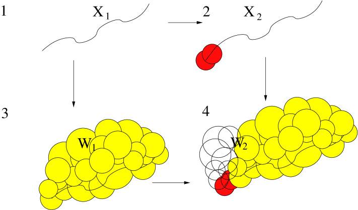
Figure 1: Given a set 1 on which analytic data is to be prescribed, if one is able to analytically extend this set by expanding as a power series in small balls (1 to 2), then this does not affect the ‘evolution’ of the original data. (the constructed data in the yellow region $W_{1}$ of 3 coincides with that in the yellow region of $W_{2}$ in 4).

Because the evolution regions are in general small, the topology of the manifolds formed by each evolution are not expected to enter the problem.

Another complication follows from combining topological considerations with the ‘Non-patching Problem’. Non-patching means that one cannot generally use a sequence of different coordinate systems that agree on their overlaps so as to construct as extensive as possible a region of data. And of course, the simple case of a sphere not being coverable by a single coordinate system, or of the speedy breakdown of normal coordinates in general relativity due to caustic formation, illustrate that one generally needs to use multiple coordinate systems in order to cover whole manifolds. This gives yet another reason why the theorem is about small patches and not whole data hypersurfaces or whole embedding manifolds.

I should also point out that, contrary to what has been hinted at in some of the literature [72], it immediately follows from the material in this section that Campbell’s conjecture has not been developed in such a way as to be able to say anything about the removal of singularities. For, the proofs are all local whereas singularities are global features, and the proofs do not concern the case with boundaries whereas singularities are often boundaries of spacetime. Moreover the approach to singularities can be rough rather than analytic [73].

Now the topology to be employed has been documented, pictures can be drawn of the three data construction methods considered in this paper and their shortcomings when applied to extended regions (Fig 2).

Figure 2: A) Picture of what generally happens in regions on which one is attempting to construct data from ‘data for the data’ prescribed on a partial boundary set $X$, for each of the 3 data construction methods discussed in this paper. The shaded region is the region $W$ for which data is being constructed by the method at each indicated stage. The obstructions indicated are: zeros $z$, points $q$ where quadratic equations cease to have real roots and points $c$ where the eliminated system is not castable into Cauchy–Kowalewskaya form. B) It is not yet clear at this stage how the shape of the region ought to be determined if one only has to contend with a bunch of isolated bad points $b$ of whichever of the above kinds. One may be tempted to form a more extensive ‘tentacled’ region $T$ which nevertheless misses out the bad points. I return to this issue of shape in Sec 7 for the timelike data surface case.

7 Difficulties if the signatures are altered

7.1 The domain of dependence property

In the GR CP, the vast majority of serious results [36, 53, 37, 38, 39, 75, 76, 40, 41, 43, 77] turn out to be entirely dependent on the signatures involved. Not only should spacetime (of whatever dimension) have precisely 1 time coordinate but also the data hypersurface must be spacelike for these methods to apply (for spacetime dimension greater than 2, see Sec 8.5). The difference between space and time is crucial in the p.d.e study of the EFE’s.

For a hyperbolic-type system to be well-posed, in addition to existence, uniqueness and continuous dependence, one requires the domain of dependence property so that the system entails a sensible notion of causality. The (future) domain of dependence ${\cal D}^{+}[A]$ of a set of points $A$ is the set of points such that all past-inextendible causal curves through each point intersect $A$. Thus, if data is given on $A$, it controls the evolution in ${\cal D}^{+}[A]$.

Note that while the domain of dependence property pertains to the hyperbolic-type system itself and not to which boundary conditions it is equipped with, it makes a huge difference to what boundary conditions are sensible for the hyperbolic-type system. If $A$ is a piece of a spatial hypersurface, then ${\cal D}^{+}[A]$ is a reasonably extensive ‘wedge’ or ‘cone’ region. But if $A$ is a piece of a timelike hypersurface, ${\cal D}^{+}[A]$ is not a reasonably extensive region because there are usually causally-connected points arbitrarily close to the timelike hypersurface from which emanate past-directed curves which do not intersect the timelike hypersurface. Thus data on a timelike hypersurface for a hyperbolic-type system do not generally control any evolution region at all. This suggests that conceptualizing in terms of such prescriptions may not make sense physically.

7.2 Conventional mathematical physics is not available

Still, one may have no choice as to what data one can know in a physical situation. The above unfortunate situation of a hyperbolic-type system with data on a timelike surface is known as a sideways Cauchy Problem. Hitherto these did not feature very often in physical situations, giving a further impasse that mathematical physics for them remains greatly undeveloped. Current results are fairly nonstandard, specialized and weak. These are usually (see Sec VI.17 of [62]; [79]) just for the standard wave equation, and depend on the shape of the data surface and often on the availability of global data for it. While Payne’s result [80] is said to be extendible to $\Box\varsigma=F\left(x_{i},t,z,\varsigma,\frac{\partial\varsigma}{\partial z}\right)$, this still falls short of the EFE’s in harmonic gauge by not being for a system, nor for a curved wave operator, nor having an $x_{i}$-dependent $F$.

If one believes in extra time dimensions (see e.g [81]), one also faces a notoriously undeveloped problem [82]: the study of ultrahyperbolic equations (see Sec VI.16 of [62] and [83]).

To appreciate this current lack of mathematical physics development, I pick out below the signature-specific features of proofs of well-posedness for the GR CP. As such proofs are widely acknowledged as essential for guaranteeing that the GR CP rests on solid foundations, their absence for other signatures surely ought to be a serious concern for the proponents of such prescriptions in the context of higher-dimensional applications.

In the study of hyperbolic p.d.e systems, comparison of the characteristic directions and the direction of integration away from a prescribed data surface is heavily entrenched in the works of Hadamard, Kirchhoff, Friedrichs, Lewy and Schauder on which the works of Stellmacher [64], Fourès-Bruhat [36, 37] and Leray [53] are based. These first works relevant to GR involve in various ways the quasilinear hyperbolic form

$${L}^{\mbox{\scriptsize CD\normalsize}}(x,\Psi_{\mbox{\scriptsize A\normalsize}},\nabla_{\mbox{\scriptsize A\normalsize}}\Psi_{\mbox{\scriptsize B\normalsize}})\nabla_{\mbox{\scriptsize C\normalsize}}\nabla_{\mbox{\scriptsize D\normalsize}}\Psi_{\mbox{\scriptsize E\normalsize}}={F}_{\mbox{\scriptsize E\normalsize}}(x,\Psi_{\mbox{\scriptsize A\normalsize}},\nabla_{\mbox{\scriptsize A\normalsize}}\Psi_{\mbox{\scriptsize B\normalsize}})$$ (19)

(where ${L}^{\mbox{\scriptsize CD\normalsize}}$ is a Lorentzian metric and both this and the function ${F}_{\mbox{\scriptsize E\normalsize}}$ are differentiable a number of times and sometimes subjected to boundedness or Lipschitz conditions depending on exactly what one is doing). Then e.g Leray’s theorem [53, 42] holds, guaranteeing all four of the well-posedness criteria. No such result is known to hold if one alters the signatures involved (evolving data on a spacelike surface with respect to a bona fide time).

A common ingredient in these studies are energy norms. (These also generalize to the Sobolev norms used in the more modern style of proof of the four well-posedness criteria for the GR CP [42, 39, 75, 41, 77]). One can see that energy norms are appropriate from simple consideration [42] of e.g the flat spacetime Klein–Gordon equation for a scalar field $\varsigma$. Given data on a bounded region $S_{0}$ of a spacelike hypersurface $\Sigma_{0}$, one can draw the future DOD ${\cal D}^{+}[S_{0}]$ (Fig 3a) which is the region affected solely by this data due to the finite propagation speed of light. One can then consider the values of $\varsigma$ and its first derivatives on $S_{t}={\cal D}^{+}[S_{0}]\cap\Sigma_{t},t>0$. Then using the construction in Fig 3, the divergence theorem and energy-momentum conservation,

$$\int_{S_{0}}{\cal T}_{AC}t^{A}t^{C}+\int_{B}{\cal T}_{AC}l^{A}t^{C}=\int_{S_{t}}{\cal T}_{AC}t^{A}t^{C}\mbox{ },\mbox{\hskip 93.95122pt}$$ (20)

and the second term $\geq 0$ provided that that $t^{A}$ is timelike and that the matter obeys the dominant energy condition:

$$-{{\cal T}^{A}}_{C}u^{C}\mbox{ is a future-directed timelike or null vector }\mbox{ }\forall\mbox{ }\mbox{future-directed timelike }u^{A}.$$ (21)

Then the definition of the energy-momentum tensor gives

$$\int_{S_{t}}\left[(\dot{\varsigma})^{2}+(\partial\varsigma)^{2}+m^{2}\varsigma^{2}\right]\leq\int_{S_{0}}\left[(\dot{\varsigma})^{2}+(\partial\varsigma)^{2}+m^{2}\varsigma^{2}\right]$$ (22)

Because each integrand is the sum of squares (each of which is nonnegative), this means that control over the data on $S_{0}$ gives control of the solution on $S_{t}$. If one alters the signatures so that one starts with a ($n$ - 1)+ 1 spacetime and adds an extra spatial dimension, then there is no analogous notion to energy (or Sobolev) norms. For, first there is generally no sideways notion of domain of dependence to make the construction. Second even if we assume the higher-d dominant energy condition holds, it would not give an inequality because the perpendicular vector $z^{A}$ in now spacelike (Fig 3). Third, we obtain a difference of squares rather than the sums in (22), so the equivalent of the energy method’s use of Sobolev norms is simply of no use to control the ‘evolution’ given the data.

Figure 3: The bucket-shaped construction for the $n$ + 1 energy norm, and its generally meaningless sideways counterpart.

7.3 The ‘Information leak Problem’

The second price to pay if one wishes to have the sideways signature Campbell–Magaard hold over an extended region is that the causal set-up is problematic. The notion that the data on this (generally local) strip controls an adjacent “evolutionary region” is generally invalidated by an ‘Information leak Problem’ (ILP), which I begin to explain in Fig 4, followed by further thought in the text below.

Figure 4: a) $\Pi$ is a $r$ + 1 (i.e timelike) hypersurface containing a data strip $W$ built by the Magaard elimination method from prescribed ‘data for the data’ on a timelike $r$-d set $x_{1}=0$. The region $\Omega$ is that part of the ($r+1$) + 1 spacetime that is supposed to be entirely controlled by $W$ i.e for which Magaard’s CK “evolution” method is valid. Typically $W$ will not cover all of $\Pi$ in the $x_{1}$-direction, so there will be nearby points like $p$ outside $W$. Consider the future null cone with apex $p$. No matter how thin in the $z$-direction one considers $\Omega$ to be, it is generally pierced by causal curves such as $\gamma$ on or in the null cone, by taking $\gamma$ to be at a sufficiently slender angle $\phi$ to $\Pi$. Thus information can leak into $\Omega$ from elsewhere than $W$, which is a contradiction. Therefore, at least in some places, $\Omega$ is arbitrarily thin in the $z$-direction. One can envisage that sometimes there will be enough points like $p$ that there is no region $\Omega$ at all. b) Suppose $X=\{x_{1}=0\}$ is spacelike and is a section of the entire hypersurface $\Pi$, and $W^{\prime}$ is the data strip built from it by the Magaard elimination method. There is now no room for points like $p$! However, typically $W^{\prime}$ will not cover all of $\Pi$ in the $x_{1}$-direction, so there will be nearby points like $q$ in the causal past of $W^{\prime}$ that are not in $W^{\prime}$. No matter how thin one considers $\Omega$ to be, it is generally pierced by causal curves $\gamma^{\prime}$ from $q$ which do not pass through $W^{\prime}$, by taking these to be at a sufficiently slender angle $\phi^{\prime}$. So again, at least in some places, $\Omega$ is arbitrarily thin and sometimes there will be enough points like $q$ that there is no region $\Omega$ at all. Small pieces of timelike hypersurfaces need not hold useful information for hyperbolic-type systems!

The ILP would be avoided whenever the data construction method happens to work globally i.e $W=\Pi$, as then there would be no points in $\Pi$ that are not in $W$. But of course, general global success of the data construction method has not been proven! One might also attempt to argue that analytic continuation (the very property that makes the CM scheme not sensible on causal grounds) could remove the ILP. However, nowhere in the proofs of Campbell’s conjecture has one proven that there exists an analytic $K_{ab}$ outside the region $W$ (and furthermore one whose values are compatible with those in $W$). Thus the data outside $W$ need not be analytic, thus analytic continuation is not generally applicable.

To attain further understanding of the ILP, I note that in case a) the ILP already occurs on the data sheet itself in the limit as the angle becomes zero. I.e in a p.d.e problem with data in this configuration, the data itself suffers from non-arbitrariness of prescription (even if the data is not assumed to be analytic). To make sense of this statement, it is helpful to consider first the simpler case of the sideways CP on a flat ($n$ - 1) + 1 plane for the $n$ + 1 flat space wave equation. What the statement then says is that general strip shapes are of no use to prescribe data on, for the data there also imply the form the data must take in the two cones (drawn as wedges in Fig 5a; see p 759 of [62]). Additionally, one may query whether one can get rid of case b). Now, assuming the sole means of influence is mediation on the null cone, further extension to form the double cone (depicted as a ‘diamond’ $D$ in Fig 5b) successfully bans points like $q$ so that case b) would not occur either. I then draw some null cones in Figs 5c and 5d to convince the reader that there are indeed no points like $p$ or $q$ as regards the sending of null signals if one adopts this ‘diamond’ construction. Moreover, I should point out that the assumption that the mediation is solely on the null cone is false if one has a massive wave equation or if there is a fluid flowing. In fact it is even false for the plain wave equation itself for the dimension of interest (4 + 1) because this assumption is based on everyday (3 + 1) intuitions about Huygens’ principle, but Huygens’ principle is false if the number of spatial dimensions is even. Thus I am not fully overcoming the ILP, but rather adopting careful causal methods to understand it as best as possible.

Figure 5: a), b) Region shapes chosen to avoid the ‘Information Leak Problem’ as best as possible. c) $r$ is not a point like the $p$ of Fig 4a): its cone does not interfere with the evolution region immediately in front of the ‘diamond’ region $D$. d) $s$ is not a point like $q$, at least as regards mediation on the null cone.

With the above insight, I now return to the more complicated case of the 4 + 1 EFE’s and what happens to the data construction part of the CM theorem on a timelike hypersurface. Starting from a set $X$ = {$x_{1}$ = const} on which ‘data for the data’ is prescribed, I choose $x_{1}$ to be a bona fide time $t$ for the 3 + 1 manifold, and I choose to build the data by evolving the ‘data for the data’ both forwards and backwards in $t$. This gives preliminarily data on a ‘doubly thick’ thin strip $W$ bounded on both sides by bad points (Fig 6a), whether due the breakdown of the eliminated system itself or of the CK proof for it. Now, given an event (i.e a point) $m$ that the data set $W$ must include, build the largest ‘diamond’ $D$ (Fig 6b) around $m$ that is free of bad points. The sides of $D$ are 3 + 1 null geodesics, which are known since the 3 + 1 metric is a known, so at least naïvely this construction can be readily made. I then note that, first, this construction rids us of the possibility of constructing data on a ‘tentacled’ set like $T$ in Fig 2B. Second, that keeping only such a $D$ entails losing a great deal of the naïve strip $W$, so this construction is ‘even more local’ than before.

Figure 6: a), b) In place of a vaguely shaped strip $W$ I will now use a ‘diamond’ $D$. c) Moreover the naïve 3 + 1 diamond $D_{4}$ may differ from the 4 + 1 diamond $D_{5}$, and points like $p$ may then reappear if one does not heed this difference.

The paragraph above about the wave equation goes to show that one would not expect this construction generally to rid us of points like $q$. The 4 + 1 EFE’s moreover give extra trouble not experienced in the wave equation example. First, 3 + 1 geodesics are not generally among the 4 + 1 ones. So in a straightforward 4 + 1 EFE model, the 3 + 1 null geodesics used to build the ‘diamond’ are in fact generally not ascribed causal physical significance, while in a general braneworld model the null 3 + 1 geodesics are only partly relevant since causal physical significance of distinct matter types is ascribed both to 3 + 1 geodesics and 4 + 1 geodesics. In either of these situations, if the ‘diamond’ $D_{5}$ made from 4 + 1 geodesics projected onto the 3 + 1 world has pieces lying outside the ‘diamond’ $D_{4}$ made from 3 + 1 geodesics (Fig 6c), then points like $p$ are re-admitted. (The case that $D_{5}$ lies entirely within $D_{4}$ would seem to be less probable than $D_{5}$ protruding somewhere or other.) Furthermore, one can not a priori use $D_{5}$ in place of $D_{4}$ since one does not a priori know what the 4 + 1 geodesics are; their form only becomes apparent once the sideways evolution has been carried out and thus the $n+1$ metric has been determined. Thus using a ‘diamond’ construction to avoid as much of the ‘Information leak Problem’ as possible for the sideways Cauchy problem for the 4 + 1 EFE’s generally entails post-evolutionary tinkering with the set on which the pre-evolutionary data is prescribed.

Second, the ‘diamond’ or ‘double-cone’ depiction betrays naïveness about what generally-relativistic null cones look like in sufficiently large regions. They can be distorted by sufficiently strong gravitation as is well-known from black hole spacetimes. Multiple weak focussing from far-apart astrophysical bodies also has an important effect on the cones as is well-known from the study of microlensing. This makes the ‘cones’ in general [85] infinitely complicated and prone to self-intersections and catastrophes such as cusp formation or refocussing to a point. In Fig 7 I illustrate how each of these effects could render a proposed ‘diamond’ flawed as regards its useability for proving CM in an extended region including a particular $m$.

Figure 7: A) One is trying to form a ‘double cone’ region $W$ enclosing $m$ by starting at two apices. B i) However, life can be cruel and one of these cones could close on itself before $m$ is surrounded by the cone. B ii) Also one of the cones could be bent away from $m$ rather than surround $m$. B iii) Even if these two effects do not quite prevent $m$ from being surrounded by a cone, they could totally or partially prevent that cone from intersecting with the other cone. In all these cases one is failing to construct a $W$ that fulfils its stated purpose of enclosing $m$. B iv) If one apex $a$ happens to have a conjugate point $a^{\prime}$ before the other cone is reached, then the original cone self-intersects. This means that if a region $W$ successfully enclosing $m$ is formed, nevertheless it could well be unsuitable for our purposes though having cusps so that $W$ is no longer of use for a CK-based proof because it is not an analytic shape. B v) Fot various higher-order catastrophes the cone could suffer from, see [86].

A way out of this complication is to resign oneself to having to accept increasingly small regions $W$ for data prescription. In the small, one could hope that the GR null ‘cones’ are well-approximated by the genuine cones of SR. Of course however the smaller the region must be before the prescription makes sense, the more stringent the word ‘local’ is in a theorem about that prescription.

As argued, the ILP can in any case not generally be avoided for the sideways CP case of CM for an extended region. I should stress that the ILP is an inherent Problem; it cannot generally be avoided by replacing Magaard’s proof with one of my proofs of Sec 5; indeed it holds quite generally for sideways Cauchy prescriptions for the $n$ + 1 EFE’s and it ought to be explored in this broader context with particular examples in a subsequent article. Moreover, of course, there is no such Problem for the bona fide CP case of CM. Thus, as in the sideways case this Problem clearly affects how one ought to precisely state whichever variant of Campbell’s theorem (see below), it is in fact not true to say that Campbell’s theorem holds regardless of signature. This can be encapsulated by saying that for the sideways case extending the word ‘local’ away from the neighbourhood notion has a series of extra connotations beyond those given in Sec 6. Namely, to avoid as much of the ILP as possible by respecting causality as best as one can in a sideways problem, that once one has a strip one ought to form a smaller ‘diamond’ out of it, that the ‘diamond’ may require amending once the evolution has been carried out, and that the ‘diamond’ may suffer additional pathologies if the region it encloses is nevertheless large so that it would need replacing with a smaller ‘diamond’. Also, because the ILP is nevertheless not fully avoided so that the possibility is opened that the embedding construction is in conflict with presupposed knowledge [the form of the metric outside the final data region $W=D(=D_{5})$]. One requires a new attitude to get round this, namely that one should re-declare that the metric was known all along only within $D$. Note that while this enables a more carefully phrased version of the theorem to survive for the sideways case, as regards the applications of this suggested in the literature, this interpretation is merely shifting the ‘ILP’ from preventing there being a theorem to tampering with its relevance to the applications proposed in the literature. This is because the original intentions of the applications are surely the wish to embed a 3 + 1 metric well-established to be a good lower-dimensional model for a sizeable patch of the 3 + 1 world (e.g a piece of Friedmann–Robertson–Walker universe large enough for the purposes of doing cosmology), so one may be straying away from having proper physical motivation if one succeeds in embedding only a tiny portion of this 3 + 1 world and subject to pretending not to know what the rest of that world looks like so as to guarantee the consistency of that embedding.

8 Conclusion and discussion of applications

8.1 The case against the Campbell–Magaard theorem

The CM theorem has been invoked as a protective theorem for the relativistic field equations of ‘noncompact Kaluza–Klein theory’ (NKK) by Romero, Tavakol and Zalaletdinov [4], especially by Wesson [5], and in a number of subsequent articles e.g [6, 7, 9, 10, 11] (see Sec 8.3). It and slight generalizations have also been invoked as protective theorems for a number of other prescriptions for the EFE’s, including the construction of brane models (see Sec 8.4). In particular Seahra and Wesson [21] presented the CM theorem in a heuristic manner as a protective theorem to underlay such constructions. While these authors were right to seek general protective theorems, they have unfortunately been let down by the CM theorem being a formal differential geometry result rather than a result that is readily useable in relativity. As I have argued in this paper, from the point of view of the study of prescriptions for relativistic field equations, the CM theorem is weak because it crucially depends on the inappropriate analytic functions, and because the protection it provides is inadequate (it just concerns existence, and with additional conditions, uniqueness, rather than full well-posedness). It is also weak to use the CM theorem for these applications because the interest is then really to have a theorem which holds in extended regions that permit meaningful astrophysical or cosmological processes to be accommodated, but the word “local” in the statement of CM cannot be straightforwardly taken to cover such a notion of extended region (Sec 6–7). This should be contrasted with the strong theorems in the GR CP and IVP literature (c.f [36, 75, 76, 41, 42]): strong theorems are for all regions, at least in many well-defined and substantial cases, like in the conformal IVP method, for adequate function spaces and supported by further well-posedness theorems. If one seeks a theorem to serve as protection in a new application, and one finds a candidate theorem in the literature, it is important to check carefully whether the candidate theorem is adequate (strong enough to provide protection) and appropriate to the context of the application. Heuristic study and presentation does not suffice and can be misleading. For example, the heuristic presentation in [21] fails to convey that the CM theorem ceases to be known to be true if its statement the analytic functions – inappropriate in the context the proposed application’s relativistic field equations – are replaced by any respectable function space.

I also described nonuniqueness difficulties in Sec 4 and non-applicability to singular manifolds in Sec 6.

8.2 There is currently no replacement protective theorem for the proposed applications

In addition to arguing against the CM theorem providing protection for the suggested applications that involve solving relativistic field equations so as to build a higher-d world that surrounds our perceived 3 + 1 spacetime from data prescribed on our apparent world, I also argue that unfortunately there are no known strong theorems that are appropriate for the study of this new and interesting possibility. To this end, I presented some general arguments in Sec 7: about how the proposed applications are causally absurd and amount to sideways Cauchy problems which have not been to date sufficiently studied. I note here that these arguments and also inconvenient locality and some forms of nonuniqueness hold against the completely general counterparts of the current schemes proposed [88] for constructing bulks from data on branes.

It is also important to consider whether other embedding theorems might be candidates for protective theorems. There are embedding theorems known for embedding into flat (Minkowski) spacetime. A difficulty with this is that it may appear to make little sense to trade the 3 + 1 EFE’s for a higher-d world with no field equations at all. Indeed, unlike in the vacuum case where CM was suggested to support NKK theory, there appear to be no proponents of any theories based on straightforward embedding into Minkowski spacetime. Note also that many extra dimensions are needed to ensure general existence, potentially compounding nonuniqueness problems. On the one hand, one has the Schläfli–Janet–Cartan–Eisenhart theorem [89], which has the advantage of requiring only (9 + 1)-d Minkowski spacetime to embed any 3 + 1 spacetime, while having the disadvantages associated with being a local theorem solely about analytic solutions. On the other hand, e.g Clarke’s theorem [90] is global and requires only $C^{3}$ metrics, but this and all other known global embedding theorems [91] involve upper bounds on minimum dimension required that are rather larger than those which arise in string theory. I should note that Katzourakis [92], contemporarily to this article, has proposed a way to sew together the final regions produced by the CM theorem. This may be of considerable interest in further developments of the topics in Sec 8.

Finally, the current absence of protective theorems for the suggested applications in the literature means that these should be treated with caution (see however Sec 8.5 for some suggestions).

8.3 Concerning the foundations of ‘noncompact Kaluza–Klein theory’

Next I consider NKK theory. The field equation for this is ${\cal R}_{AB}=0$. The relevance of CM would then be [5] 1) as a guarantee that each 3 + 1 GR solution can be represented by a 4 + 1 solution of ${\cal R}_{AB}=0$. 2) Wesson then claims that NKK theory based on ${\cal R}_{AB}=0$ is a geometrization of completely general matter, so that it “realizes Einstein’s dream” of ‘transposing the basewood’ of the energy-momentum tensor into the ‘marble’ of geometry.

In answer to 1), I recollect also that before CM resurfaced in the literature, Wesson already postulated ${\cal R}_{AB}=0$ but admitted [12, 13] that it was a choice among the ${\cal G}_{AB}={\cal T}_{AB}$. It has subsequently been argued and asserted [4, 5, 6, 7, 10, 11] both that CM both provides support for and specifically picks out ${\cal R}_{AB}=0$. However, I have pointed out in this article that CM is not suited to provide support. Furthermore, CM is not a valid selection criterion for ${\cal R}_{AB}=0$, because there is an analogous statement for cosmological constants or many kinds of matter in place of the zero left hand side (see e.g [20]). Thus a return to the earlier position that ${\cal R}_{AB}=0$ is a choice would seem necessary.

Note however that 2) may be interpreted as advocating further, distinct support for ${\cal R}_{AB}=0$. I.e that it is the entirely geometrical character of ${\cal R}_{AB}=0$ itself that is special. But I argue below that as a prospective geometrization or Einstein-like unified field theory (UFT), NKK theory is not established to have several useful features that KK theory proper possesses. In KK theory proper, a specific known fundamental matter field, the electromagnetic potential, and its corresponding field equations (Maxwell’s equations) are geometrized (alongside an unobserved scalar with its field equation). My argument is that the slanted words above are surely a significant part of what a geometrization or a UFT should be about. I.e the offering of new insights about known fundamental fields through representing their field equations in a novel geometrical way. In contrast, NKK theory is usually considered only to include a scalar. Although one might [5] include a more general vector field than the electromagnetic potential in addition, the corresponding field equation is clearly not, on inspection, that of any known vector field of nature. Indeed, the 3 + 1 matter in noncompact KK theory is to be interpreted phenomenologically. In all fairness, Wesson is well aware that more degrees of freedom would be required (see [27, 93]) before a full physical picture could emerge from such a scheme. But it should be pointed out that there are two somewhat distinct further contentious issues in addition to the issue of counting degrees of freedom.

A) By including fields more general than the electromagnetic potential, but not having enough degrees of freedom to discern an electromagnetic contribution from whatever else one hopes to include, one appears to be decreasing the value of the theory as a geometrization or UFT by losing insights specific to each fundamental field. For example a great deal of quantum-mechanical success (QED, Weinberg–Salam theory, QCD) stems from quantizing discernible fundamental fields. Completely switching to a NKK view of the world with its capacity only to include phenomenological matter would effectively amount to choosing to ignore these successes. Thus it is not just a case of requiring more degrees of freedom, but also of requiring to supplant the phenomenological interpretation of the matter itself (or, as a long shot, of finding a means of recovering quantum mechanical successes from within NKK).

B) If one attempted to argue (despite the strong caveats above) that the CM theorem is itself meant to have something to do with the geometrization in NKK theory, it should be noted that the CM theorem is a geometrical guarantee that given a 3 + 1 solution, there exists a unique solution of ${\cal R}_{AB}=0$. But such an application has a further undesirable feature: it is at the level of re-representing solutions piecemeal rather than at the level of finding and using a new geometrical representation of field equations, which would be most likely to be what is required to have a useful geometrization or UFT.

8.4 Comments about claimed applications in the study of embeddings and braneworlds

Despite the CM theorem being claimed to be an underlying result in a number of papers, I note that in fact it does not appear to be used directly in any of the constructions of specific examples contained within these. Rather, the messy Magaard part of the prescription is simply ignored and replaced by neater methods which often turn out to be among the cruder simplifications of the conformal IVP method [49, 41, 50]. Unlike what is claimed e.g in [21], without such a specific prescription, all one is applying to modern scenarios is the standard embedding mathematics associated with the split EFE’s, and not an ‘old but little known result’.

Specifically, when it comes down to finding particular examples, the simplifying assumption $K_{ab}=0$ has been used a lot [4, 16, 17, 18, 29, 21]. In the GR IVP, this is the time-symmetric condition and is considered bereft of much generality [68, 45, 46]. In the current application it is rather a ‘space-symmetric’ condition as regards the large extra spatial dimension, but is likewise bereft of much generality.

The somewhat more general assumption $K_{ab}=Ch_{ab}$ (for $C$ constant on the 3 + 1 hypersurface one starts on) is used in [17, 9, 19]. I note that this is a subcase of $K=C$, which is the constant mean curvature condition, well-known in the IVP literature to simplify the system by decoupling (2) from (4) [49, 41]. A subcase of this is the maximal condition [48]: $K=0$, which of course also generalizes the above simplifying assumption $K_{ab}=0$, and which emerges in [29] as the desired condition for that application (establishing existence of embeddings that are also harmonic maps). I suggest that if one is interested in more examples along the lines of the above papers, then a fruitful place to look is the embedding of hypersurfaces or branes of constant mean curvature. For, the above decoupling technique for the constraint system carries through regardless of signature. As the constraint system changes fundamentally in character in switching signature, specific details would have to be worked out afresh for the new timelike hypersurface situation.

In the case of (thin EFE-based) braneworlds, the junction condition

$$K_{ab}=-\frac{1}{2}\left(Y_{ab}-\frac{Y}{3}h_{ab}\right)$$ (23)

arises [24], where $Y_{ab}=S_{ab}-\lambda h_{ab}$ consists of the discontinuous contribution to the on-brane matter energy-momentum $S_{ab}$ and the brane tension $\lambda$. Now, this imposition will usually mean a conflict between what are knowns and unknowns in Magaard’s method and what on-brane matter is of interest to the theorist. So Magaard’s method will often not be suitable. [21] and [22] acknowledge this but still claim support from CM while adopting prescriptions for the constraints other than the one for which Magaard’s proof holds. Both these works also claim that other prescriptions for the constraints can be solved just because they can be declared to contain more degrees of freedom than equations. This is non sequitur. It suffices to note that the system $x+y+z=0;x+y+z=1$ has no solutions even if $x$, $y$ and $z$ are all declared to be free. Thus one needs to specifically check whether a given prescription entails existence.

It should also be noted that imposing (23) reduces the scope of what each ansatz can include. For example, my suggested $K=C$ ansatz implies $Y=C$. Thus this ansatz will preclude many types of matter, although it will permit investigation of embeddings of interesting cases such as vacuum, phenomenological radiation and fundamental electromagnetism.

8.5 Some suggested routes for progress

I finish by suggesting several routes forward from this paper. These are more modest than recent claims that the CM theorem is a completely general result that meaningfully underlays theories such as NKK or bulks constructions for braneworld scenaria. First, as regards Magaard’s method or either of my methods in this paper, it is after all correct to use them free of all the signature problems and proof aspects (analyticity and whatever kind of locality), as alternative techniques for the bona fide GR IVP.

Second, as regards the difficulties uncovered with the general study of braneworlds, there are several ways forward. One should distinguish between two distinct problems to study: on the one hand the bona fide dynamical computation of how a given and consistent initial brane-bulk configuration evolves, and on the other hand direct attempts to make predictions within a 4 + 1 ontology given our observations of the apparent 3 + 1 world. In the former case, one proceeds by constructing appropriate 4 + 0 initial data [96, 84], and then asks what the 4 + 1 GR Cauchy problem has to say about what then happens to the brane(s) and to the immediately-surrounding bulk. Such a study might also be simpler [84] if done for nice smooth thick branes [25] rather than for the more habitually-studied arbitrarily-thin brane models. But if faced with the aspects only resolvable by the latter case, one may have to acknowledge that braneworlds giving rise to p.d.e problems that are not known to be well-posed. This would mean that giving definite answers to what life is like on a brane would be much harder than making comparable statements in ordinary 3 + 1 GR. I do not suggest that one should jump too quickly onto the interpretation and nonstandard analysis of this, but rather to consider whether any optimal reformulations might arise by good use of gauge freedom and/or defining new variables [98].

Third, I note that sufficiently symmetric problems effectively involve a 2-dimensional reduced bulk space. This special case includes as a subcase the embedding of homogeneous cosmologies for which the bulk metric to be a function of a time coordinate $t$ and a bulk coordinate $z$. This subcase involves a reduced 1 + 1 bulk whereupon there is no longer a geometrical distinction between a CP and a sideways CP (Fig 8). Then an analogue notion of domain of dependence, of Leray form, of energy integral etc, make sense in the reduced sideways problem, alongside yet other techniques specific to such ‘two independent variable’ p.d.e’s (see Ch 5 of [62]). So at least for this subcase, protective theorems are available. I will present this in detail elsewhere. Another subcase are embeddings of static spherically symmetric models for which the bulk metric is to be a function of a radial coordinate $r$ and a bulk coordinate $z$. This subcase involves solving entirely spatial (2 + 0) bulk equations so the above comments about solving spacetime equations are no longer applicable; on the other hand this is at the price of no dynamics being included.

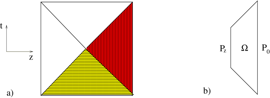
Figure 8: For effective 1 + 1 problems, space and time do not have a distinct formal status. This is because space and time are now equally complicated so one can describe $t$ as $t(x)$ just as well as one can describe $x$ as $x(t)$. a) The vertically striped region is now equivalent under rotation to the horizontally striped region. b) Then it may be interpreted that $\Omega$ is controlled by $P$ and that $\Omega$ constitutes a ‘bucket-shaped’ construction which may be used in a direct analogue of energy norm proofs.

Note that while such studies would be of some use toward bulk construction prescriptions (indeed to date the works [88] are restricted to static models and brane cosmology is restricted to at most homogeneous anisotropic models) it would be strictly limited to highly-symmetric models. Thus such work would not constitute anything like the same level of protection as was claimed from the completely general CM theorem prior to this article.

Acknowledgments

I thank Reza Tavakol, Carlos Romero, Julian Barbour, James Vickers, Nikolaos Katzourakis and especially Malcolm MacCallum for comments and discussions. I thank Peterhouse Cambridge and the Killam Foundation for funding the next stage of my career.

References

- [1]
- [2] J. Campbell, A course of Differential Geometry (Clarendon, Oxford 1926).
- [3] L. Magaard, “Zur einbettung riemannscher Raume in Einstein–Raume und konformeuclidsche Raume” (PhD Thesis, Kiel 1963).
- [4] C. Romero, R. Tavakol and R. Zalaletdinov, Gen. Rel. Grav. 28 365 (1996).
- [5] P.S. Wesson, Space-Time-Matter (World Scientific, Singapore 1999).
- [6] H-Y. Liu and P.S. Wesson, Gen. Rel. Grav. 30 509 (1998); H.L. Carrion, M.J. Reboucas and A.F.F. Teixera, J. Math. Phys. 40 4011 (1999), gr-qc/9904074; A.G. Agnese and M. La Camara, Nuovo Cim. B115 119 (2000), gr-qc/0002028; P.S. Wesson, H-Y. Liu and S.S. Seahra, Astron. Astrophys. 358 425 (2000), gr-qc/0003012; F. Darabi and P.S. Wesson, Phys. Lett. B527 1 (2002), gr-qc/0003045; H-Y. Liu and P.S. Wesson, J. Math. Phys. 42 4963 (2001), gr-qc/0104009; P.S. Wesson and H-Y. Liu, Int. J. Mod. Phys. D10 905 (2001), gr-qc/0104045; P.S. Wesson, J. Math. Phys. 43 2423 (2002), gr-qc/0105059; A.P. Billyard and W.N. Sajko, Gen. Rel. Grav. 33 1929 (2001), gr-qc/0105074; H-Y. Liu and P.S. Wesson, Astrophys. J. 562 1 (2001), gr-qc/0107093; S.S. Seahra and P.S. Wesson, Class. Quant. Grav. 19 1139 (2002), gr-qc/0202010; P.S. Wesson, Class. Quant. Grav. 19 2825 (2002), gr-qc/0204048; H-Y. Liu and Q. Zhang, J. Math. Phys. 43 4904 (2002), gr-qc/0206036; B. Wang, H-Y. Liu and L. Xu, Mod. Phys. Lett. A19 449 (2004), gr-qc/0304093; P.S. Wesson, Gen. Rel. Grav. 35 111 (2003); P.S. Wesson, gr-qc/0309100; J. Ponce de Leon, Gen. Rel. Grav. 36 1335 (2004), gr-qc/0310078; T. Liko, J.M. Overduin and P.S. Wesson, Space Sci. Rev. 110 337-357 (2004), gr-qc/0311054; B. Mashhoon and P.S. Wesson, Class. Quant. Grav. 21 3611 (2004), gr-qc/0401002; J. Ponce de Leon and P.S. Wesson, gr-qc/0402046; J.E. Madriz Aguilar and M. Bellini, hep-th/0406268; P.S. Wesson, gr-qc/0407038; J.E. Madriz Aguilar and M. Bellini, gr-qc/0408054.
- [7] T. Liko, J.M. Overduin and P.S. Wesson, Space Sci. Rev. 110 337 (2004), gr-q/0311054.
- [8] New Scientist 20 November 2004, p. 30.
- [9] E. Anderson and J.E. Lidsey, Class. Quant. Grav. 18 4831 (2001), gr-qc/0106090.
- [10] F. Dahia, E.M. Monte and C. Romero, Mod. Phys. Lett. A18 1773 (2003), gr-qc/0303044.
- [11] J.J. Figueiredo and C. Romero, gr-qc/0405079.
- [12] P.S. Wesson, Gen. Rel. Grav. 16 193 (1984).
- [13] P.S. Wesson, Gen. Rel. Grav. 22 707 (1990).
- [14] P.S. Wesson, Astrophys. J. 394 10 (1992); J. Ponce de Leon and P.S. Wesson, J. Math. Phys. 33 3883 (1992); P.S. Wesson, Gen. Rel. Grav. 16 193 (1994); P.S. Wesson et al, Int. J. Mod. Phys. A11 3247 (1996); J.M. Overduin and P.S. Wesson, Phys. Rept. 283 303 (1997), gr-qc/9805018.
- [15] H-Y. Liu and J.M. Overduin Astrophys. J. 538 386 (2000), gr-qc/0003034; J.M. Overduin, Phys. Rev. D62 102001 (2000), gr-qc/0007047.
- [16] J.E. Lidsey, C. Romero and R. Tavakol, Mod. Phys. Lett. A12 2319 (1997).
- [17] J.E. Lidsey, C. Romero, R. Tavakol and S. Rippl, Class. Quantum Grav. 14 865 (1997), gr-qc/9907040.
- [18] J.E. Lidsey, Phys. Lett. B417 33 (1998); J.E. Lidsey, Phys. Rev. D62 083515 (2000), hep-th/0007014.
- [19] F. Dahia and C. Romero, J. Math. Phys. 43 5804 (2002), gr-qc/0109076.
- [20] E. Anderson, F. Dahia, J.E. Lidsey and C. Romero, J. Math. Phys 44 5108 (2003), gr-qc/0111094.
- [21] S.S. Seahra and P.S. Wesson, Class. Quantum Grav. 20 1321 (2003), gr-qc/0302015.
- [22] F. Dahia and C. Romero, Class. Quantum Grav. 21 927 (2004), gr-qc/0308056.
- [23] L. Randall, R. Sundrum, Phys. Rev. Lett. 83 3370 (1999), hep-ph/9905221; L. Randall, R. Sundrum, Phys. Rev. Lett. 83 4690 (1999), hep-th/9906064.
- [24] T. Shiromizu, K. Maeda, M. Sasaki, Phys. Rev. D62 024012 (2000), gr-qc/9910076; R. Maartens, Living Reviews Relativity 7 (2004), gr-qc/0312059.
- [25] F. Bonjour, C. Charmousis and R. Gregory, Phys. Rev. D62 083504 (2000), gr-qc/0002063; E. Kiritsis, N. Tetradis and T. Tomaras; JHEP 0108 012 (2001), hep-th/0106050; S. Kobayashi, K. Koyama and J. Soda, Phys. Rev. D65 064014 (2002), hep-th/0107025; P. Mounaix and D. Langlois, Phys. Rev. D65 103523 (2003), gr-qc/0202089; C. Barceló and A. Campos Phys. Lett. B563 217 (2003), hep-th/0206217; R. Mansouri, M. Borhani and S. Khakshournia, hep-th/0301228; K. Ghoroku and M. Yahiro, hep-th/0305150; D. Bazeia, C. Furtado and A.R. Gomes, JCAP 0402 002 (2004), hep-th/0308034; S.S. Seahra, Phys. Rev. D68 104027 (2003), hep-th/0309081; D. Bazeia and A.R. Gomes, JHEP 0405 012 (2004) 012, hep-th/040314; J. Vinet and J.M. Cline, hep-th/0406141; R. Koley and S. Kar, hep-th/0407159; J. Vinet, hep-th/0408082.
- [26] K.A. Bronnikov, H. Dehnen and V.N. Melnikov, Phys. Rev. D68 024025 (2003) gr-qc/0304068.
- [27] M.D. Maia, gr-qc/9512002.
- [28] F. Dahia and C. Romero, J. Math. Phys. 43 3097 (2002), gr-qc/0111058.
- [29] S. Chervon, F. Dahia and C. Romero, Phys. Lett. A326 171 (2004), gr-qc/0312022.
- [30] F. Dahia and C. Romero, to appear in Essays in honor to Mario Novello, gr-qc/0305066.
- [31] J.M Sanchez-Ron, in Studies in the History of GR, ed. J. Eisenstaedt and A.J. Kox (Birkhauser, Boston 1992).
- [32] J. Stachel, in Studies in the History of GR, ed. J. Eisenstaedt and A.J. Kox (Birkhauser, Boston 1992).
- [33] H.F. Goenner, in General Relativity and Gravitation ed. A. Held (Plenum, New York 1980).
- [34] G. Darmois, Comptes Rendus 176 646; 731 (1923); G. Darmois, Annales de Physique 1 5 (1924).
- [35] G. Darmois, Mem. Sci. Math. 25 (1927).
- [36] Y. Fourès-Bruhat, Acta Mathematica 88 141 (1952).
- [37] Y. Fourès-Bruhat, J. Rat. Mech. Anal. 5 951 (1956).
- [38] Y. Bruhat, in Gravitation: an introduction to current research, ed. L. Witten (Wiley, New York, 1962).
- [39] S.W. Hawking and G.F.R. Ellis, The Large-Scale Structure of Space-Time (Cambridge University, Cambridge 1973).
- [40] A.E. Fischer and J.E. Marsden, in General Relativity: an Einstein Centenary Survey ed. S.W. Hawking ans W. Israel (Cambridge University, Cambridge 1979).
- [41] Y. Choquet-Bruhat and J.W. York, in General Relativity and Gravitation ed. A. Held, vol. 1 (Plenum, New York, 1980).
- [42] R.M. Wald General Relativity (University of Chicago, Chicago, 1984).
- [43] H. Friedrich and A.D. Rendall, Lect. Notes Phys. 540 127 (2000), gr-qc/0002074.
- [44] A.D. Rendall, Living Rev. Rel. 5 6 (2002), gr-qc/0203012.
- [45] G.B. Cook, Living Rev. Rel. 3 5 (2000), gr-qc/0007085.
- [46] T.W. Baumgarte and S.L. Shapiro, Phys. Rept. 376 41 (2003), gr-qc/0211028.
- [47] 50 years of the Cauchy Problem in General Relativity, in honour of Y. Choquet-Bruhat, ed. P. Chruściel and H. Friedrich.
- [48] A. Lichnerowicz, J. Math. Pures Appl. 23 37 (1944).
- [49] J.W. York, Phys. Rev. Lett. 26 1656 (1971); 28 1082 (1972); J.W. York, J. Math. Phys. 14 456 (1973).
- [50] I collected some of these simplifications for th GR IVP in Appendix C of [71].
- [51] J.E. Campbell, Proceedings of the London Mathematical Society 20 1 (1920); 21 317 (1922); 22 92 (1923).
- [52] See the preface of [2].
- [53] J. Leray, Hyperbolic Differential Equations (The Institute For Advanced Study, Princeton 1952).
- [54] R. Arnowitt, S.Deser and C.W. Misner, in Gravitation: an Introduction to Current Research ed L. Witten (Wiley, New York 1962); P.A.M. Dirac, Lectures on Quantum Mechanics (Yeshiva University, NY, 1964).
- [55] K.F. Gauss, Disquisitiones generales circa superficies curvas, Werke 4 217 (1827); D. Codazzi, Annali Ser. 3 2 269 (1868); It is also worth mentioning the big transition in notation in the study of these [e.g c.f the older G. Darboux, Theorie des Surfaces (Gauthier–Villars, Paris 1894-1896) or L. Bianchi, Lezoni di geometria differenziale (Spoerri, Pisa 1902-1903) against the newer L.P. Eisenhart Riemannian Geometry (Princeton University, Princeton 1926)]. Campbell’s approach [99] to differential geometry was based on studying these older treatises. Although he would have had much of the right sort of understanding from these texts, he was unaware that what he was dealing with in his book was the same very same situation but in the new (but not as yet widely known) notation, so his understanding was squandered.
- [56] D. Hilbert, Königliche Gesellscaft der Wissenschaften zu Göttingen Mathematisch-Physikalische Klasse Nachrichten 55 (1917); some of these results were also obtained in E. Vessiot, Acad. Sci. (Paris) Comptes Rendus 166 349 (1918).
- [57] T. Levi-Cività, Acad. dei Lencei Rendicanti 26 381 (1917).
- [58] G.D. Birkhoff and R.E. Langer, Relativity and Modern Physics (Harvard University, 1923).
- [59] K. Lanczos, Phys Z. 23 537 (1923). Note that Lanczos was unaware of much of the rest of the work in this section and re-derived much of it at a somewhat later date.
- [60] The literature of the development of the Cauchy–Kowalewskaya theorem is carefully listed in the first chapter of [61].
- [61] J. Hadamard, Lectures on Cauchy’s problem in linear partial differential equations (Yale University, New Haven and Oxford University, Oxford 1923).
- [62] R. Courant and D. Hilbert, Methods of Mathematical Physics Volume II (Wiley Classics Edition, New York 1989).
- [63] E. Cartan, Bull. Soc. Math. France 59 88 (1931).
- [64] K. Stellmacher, Math. Ann. 115 136 (1938).
- [65] L. Smarr and J.W. York, Phys. Rev. D17 1945 (1978).
- [66] See T. de Donder, in Mem. Sci Math. 8 (1925) and references therein.
- [67] K. Lanczos, Ann. Phys. 13 621 (1922).
- [68] Sources of gravitational radiation, ed. L. Smarr (Cambridge University, Cambridge 1979); Frontiers in Numerical Relativity ed. C.R. Evans, L.S. Finn and D.W. Hobill (Cambridge University, Cambridge 1989).
- [69] B.S. DeWitt, Phys. Rev. 160 1113 (1967).
- [70] B. Greene, lectures given at TASI96, hep-th/9702155; L. Susskind, hep-th/0302219; M.R. Douglas, JHEP 0305 046 (2003), hep-th/0303194.
- [71] E. Anderson, “Geometrodynamics: spacetime or space?” Ph.D Thesis, University of London (2004).
- [72] H-Y. Liu and P.S. Wesson, Astrophys.J. 562 1-6 (2001), gr-qc/0107093; S.S. Seahra and P.S. Wesson, Class. Quant. Grav. 19 1139 (2002), gr-qc/0202010.
- [73] C.J.S. Clarke, The Analysis of Space-Time Singularities (Cambridge University Press, Cambridge 1993).
- [74] R.L. Bryant, S.S. Chern, R.B. Gardner, H.L. Goldschmidt and P.A. Griffiths, Exterior differential systems (Springer-Verlag, New York, 1999).
- [75] T.J.R. Hughes, T. Kato and J.E. Marsden, Arch. Rat. Mech. Anal. 63 273 (1976).
- [76] Y. Choquet-Bruhat, in Differential Geometry and Relativity , ed. M. Cahen and M. Flato (D. Reidel, Dordrecht 1976).
- [77] S. Klainerman and I. Rodnianski, math.AP/0109173.
- [78] See especially A.N. Tikhonov and V.V. Arsenin Solutions of Ill Posed Problems (Wiley, New York 1977).
- [79] F. John, Commun. Pure Appl. Math. 13 551 (1960); H.A. Levine and L.E. Payne, Office of Naval Research Report (1985); K.A. Ames and V. Isakov, J. Math. Anal. Appl. 156 597 (1991); Lop Fat Ho, C.R. Acad. Sci. Paris Ser. I Math. 302 443 (1986); V. Isakov, Comm. Pure Appl. Math 39 747 (1986); Comm. Partial Differential Equations 14 465 (1989); K.A. Ames and B. Straughan, Non-standard and Improperly Posed Problems (Academic, San Diego 1997).
- [80] L.E. Payne, Applicable Analysis 19 63 (1985).
- [81] See, for example, A.D. Sakharov, Zh. Eksp. Teor. Fiz. 87 375 (1984); C. Vafa, Nu. Phys. B469 403 (1996); C.M. Hull, J. High Energy Phys. 7 21 (1998); C.M. Hull and R.R. Khuri, Nu. Phys. B536 219 (1998); C.M. Hull, in Proceedings of Mathematical Sciences beyond the Second Millennium, hep-th/9911080; M. Chaichian and A.B. Kobakhidze, Phys. Lett. B488 117 (2000), hep-th/0003269.
- [82] M. Tegmark, Class. Quantum. Grav. 14 L69 (1997), gr-qc/9702052; S.F. Hewson, hep-th/9908209.
- [83] F. John, Duke Math. J. 4 300 (1938); M.M. Lavrent’ev, V.G. Romanov and S.P Sisatskii, available in English translation as Ill-Posed Problems of Mathematical Physics and Analysis, Translations of Mathematical Monographs 64 (American Mathematical Society, Providence, Rhode Island 1986).
- [84] E. Anderson and R. Tavakol, gr-qc/0309063.
- [85] R. Tavakol and G.F.R. Ellis, Phys. Lett. B469 37 (1999), hep-th/9908093.
- [86] J.M. Stewart, Advanced General Relativity (Cambridge University, Cambridge 1991).
- [87] H. Stephani, D. Kramer, M.A.H. MacCallum, C. Hoenselaers and E. Herlt, Exact Solutions to Einstein’s Field Equations Second Edition (Cambridge University, Cambridge 2003).
- [88] A. Chamblin, H.S. Reall, H. Shinkai and T. Shiromizu, Phys. Rev. D63 064015 (2001), hep-th/0008177; T. Wiseman, Phys. Rev. D65 124007 (2002), hep-th/0111057; M. Visser and D.L. Wiltshire, Phys. Rev. D67 104004 (2003), hep-th/0212333.
- [89] This work follows a conjecture by L. Schläfli, Ann. di Mat. 5 170 (1871). It was proven for positive-definite metrics in M. Janet, Ann. Soc. Polon. Math. 5 38 (1926); E. Cartan, Ann. Soc. Polon. Math. 6 1 (1927). It was generalized to the indefinite case in L.P. Eisenhart, Riemannian Geometry (Princeton University, Princeton 1949 edition).
- [90] C.J.S. Clarke, Proc. Roy. Soc. Lond. A314 17 (1970).
- [91] J. Nash, J. Ann. Math. 63 20 (1956); R.E. Greene, Memoirs Amer. Math. Soc. 97 1 (1970); M. Gunther, Math. Nachr. 144 165 (1989).
- [92] N.I. Katzourakis, math-ph/0407067; math.DG/0411630.
- [93] A.A. Coley, Astrophys. J. 427 585 (1994).
- [94] E. Witten, Nu. Phys. B186 412 (1981).
- [95] E. Anderson and R. Tavakol, in preparation.
- [96] K. Nakao, K. Nakamura and T. Mishima, Phys. Lett. B564 , 143 (2003), gr-qc/0112067; K. Nakamura, K. Nakao and T. Mishima, Progress of Theoretical Physics Supplement 148 Brane World: New Perspective in Cosmology , gr-qc/0302058; T. Shiromizu and M. Shibata, Phys. Rev. D62 127502 (2000), hep-th/0007203; E. Anderson, gr-qc/0402010, to appear in proceedings of Rio de Janeiro 2003 Marcel Grossman meeting.
- [97] A. Chamblin and G.W. Gibbons, Phys. Rev. Lett. 84 1090 (2000), hep-th/9909130; M. Sasaki, T. Shiromizu and K-i. Maeda, Phys. Rev. D62 024008 (2000), hep-th/9912233.
- [98] E. Anderson and R. Tavakol Class. Quant. Grav. 20 L267 (2003), gr-qc/0305013 discusses some reformulations of the sideways problem for the EFE’s. For an idea of the scope and usefulness of GR CP reformulations, see e.g [43] and [46].
- [99] J.E. Campbell’s obituary, in Proceedings of the London Mathematical Society 23 1xx (1924).