Signaling, Entanglement, and Quantum Evolution Beyond Cauchy Horizons

Abstract

Consider a bipartite entangled system half of which falls through the event horizon of an evaporating black hole, while the other half remains coherently accessible to experiments in the exterior region. Beyond complete evaporation, the evolution of the quantum state past the Cauchy horizon cannot remain unitary, raising the questions: How can this evolution be described as a quantum map, and how is causality preserved? What are the possible effects of such nonstandard quantum evolution maps on the behavior of the entangled laboratory partner? More generally, the laws of quantum evolution under extreme conditions in remote regions (not just in evaporating black-hole interiors, but possibly near other naked singularities and regions of extreme spacetime structure) remain untested by observation, and might conceivably be non-unitary or even nonlinear, raising the same questions about the evolution of entangled states. The answers to these questions are subtle, and are linked in unexpected ways to the fundamental laws of quantum mechanics. We show that terrestrial experiments can be designed to probe and constrain exactly how the laws of quantum evolution might be altered, either by black-hole evaporation, or by other extreme processes in remote regions possibly governed by unknown physics.

1. Overview

Standard proofs that non-local Bell correlations bellcorr between parts of an entangled system cannot be used to acausally signal (transfer information) rely on quantum evolution being everywhere unitary. However, as Hawking hawkingnonunit first pointed out when he gave examples of non-unitary but causal maps for evaporating black holes, unitarity, a sufficient but not a necessary condition for causality, may break down in the late stages of black-hole evaporation. In this paper we ask: When entangled systems partly cross the event horizons of evaporating black holes (or Cauchy horizons of other, more general naked singularities) and partly remain coherently accessible to experiments outside, what constraints on their non-unitary, and possibly nonlinear quantum evolution would ensure causality? and: Can signaling (acausal) evolution be detected at large distances if it indeed does take place under the extreme conditions near naked singularities and evaporating black-hole interiors?

It turns out, as we will show below, that linearity (along with probability conservation and locality) is sufficient to preserve causality; acausal signaling is possible only with nonlinear maps. Nonlinear generalizations of quantum mechanics and their implications for measurement theory and causality have been discussed by many authors nlrefs ; it is not our goal in this paper to contribute to these formal developments. We adopt the conservative position that at most a minimal generalization of quantum theory—namely one that allows for the possibility of nonlinear quantum maps while keeping the rest of the formalism intact—is necessary to understand the implications of non-standard quantum dynamics for entangled states. There is, of course, no experimental evidence for quantum nonlinearity under local laboratory conditions weinberg ; however, whether linearity continues to hold under extreme conditions such as those inside evaporating black-holes is a question yet to be decided by experiment. We will discuss a simple terrestrial experiment which can probe this question.

Our goal is to show two things: (i) Although any nonlinearity in quantum mechanics under ordinary laboratory conditions is essentially ruled-out by local experiments, late stages of black-hole evaporation, and, more generally, naked singularities, are environments where conditions are extreme enough (and the local physics is sufficiently uncertain) to raise the possibility of quantum nonlinearity. And (ii) one can probe quantum physics in these remote extreme regions of spacetime by local terrestrial experiments, such as by the experiment we propose in detail below. The main argument of this paper consists of explaining why (a) the proposed experiment is a novel test of certain generic violations of the linearity of quantum mechanics at large distances, (b) that such violations at-a-distance, though unlikely, are nevertheless not ruled out by existing local experiments, and (c) that therefore the proposed experiment is a compelling test, since the laws of quantum evolution under extreme conditions in remote regions (such as in black-hole interiors, near naked singularities, and other regions where the laws remain untested by observation, for example, beyond our cosmological event horizon) might be nonlinear.

The experiment we outline in detail in this paper does not require extremely high energies, sensitivity, or other ultra-improved technologies to perform: The “proof of concept” for our proposed experiment has already been successfully demonstrated by Mandel et. al. mandeletal more than a decade ago. Our proposed modification of the Mandel experiment can be performed today, with a small investment of research effort, by any of the dozens of quantum optics laboratories around the world.

Throughout the paper, our focus will be on complete black-hole evaporation as the most likely possible source of a signal, and the most plausible target, for our experiment. In fact, in an attempt to restore the unitarity of the evaporation process, Horowitz and Maldacena HM recently proposed a boundary-condition constraint for the final quantum state of an evaporating black hole at its singularity. Gottesman and Preskill GP have argued that the proposed constraint must lead to nonlinear evolution of the initial (collapsing) quantum state. Here we will show that this evolution is a signaling quantum map, detectable outside the event horizon with the entangled probe we propose, and making the Horowitz-Maldacena proposal subject to terrestrial tests. Independently of this specific example, our ultimate goal is to convince the reader that the trans-horizon Bell-correlation experiment we are proposing is worth doing. The black-hole emphasis of our argument is grounded in the view that black-hole evaporation is the most likely known candidate for new physics that involves a breakdown in the linearity of quantum mechanics. Naturally, one could also argue for “unknown physics” elsewhere in our future lightcone as a potential target for the experiment; we foresee, however, that many readers may find this argument less persuasive.

2. Black-hole evaporation and non-standard quantum mechanics

Why expect the experimentally well-established law of unitary evolution to break down during black-hole evaporation? Consider, for definiteness, a pure quantum-field state which gravitationally collapses to form an evaporating Schwarzschild black hole (Fig. 1). Initially given by $|\Psi_{0}\rangle$ on the (partial) Cauchy surface $\Sigma_{0}$ in Fig. 1, the state evolves unitarily (at least in semiclassical gravity) during and after gravitational collapse: at any intermediate time slice

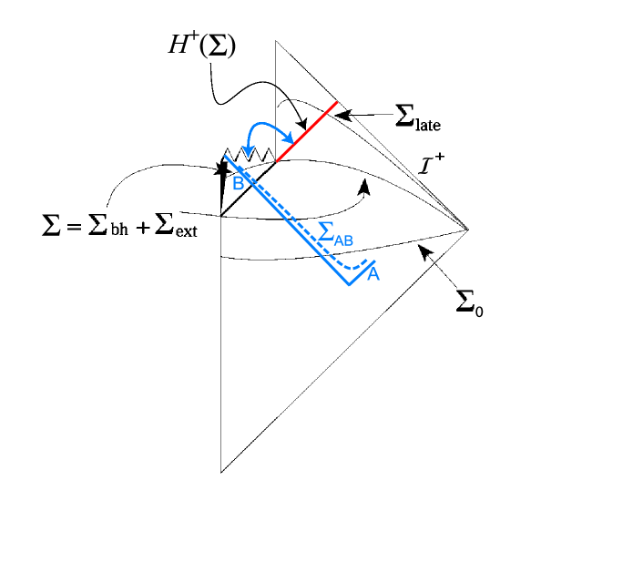
Figure 1: Conformal diagram illustrating the causal structure of a spacetime with an evaporating black hole (vertical lines on the left depict the axes of rotational symmetry). [The causal geometry illustrated by the superimposed blue drawing refers to the paragraph immediately preceding Sect. 4 below.] The spacelike hypersurface $\Sigma_{0}$ passes through the collapsing star before the black hole has formed, $\Sigma$ is a surface through the black hole just before it evaporates, and $\Sigma_{\rm late}$ is a surface at late times, after complete evaporation. The red line illustrates the Cauchy horizon $H^{+}(\Sigma)$ for $\Sigma$ or $\Sigma_{0}$; it is the future null cone of the “point” (really a singularity) of complete evaporation. Because evaporation is largely thermal, quantum evolution through $H^{+}(\Sigma)$ from the time slice $\Sigma_{0}$ to the slice $\Sigma_{\rm late}$ cannot be described as a unitary map.

$\Sigma$, it can be written as $|\Psi_{\Sigma}\rangle=U_{\Sigma\,\Sigma_{0}}|\Psi_{0}\rangle$, where $U_{\Sigma\,\Sigma_{0}}$ is the unitary time evolution operator acting on the Fock space of field states. An external observer in the asymptotically flat region outside the event horizon has no causal communication with the interior $\Sigma_{\rm bh}$; she would describe the state of the quantum field by the reduced density matrix

$$\rho_{\rm ext}={\rm Tr}_{\Sigma_{\rm bh}}\,|\Psi_{\Sigma}\rangle\,\langle\Psi_{\Sigma}|\;$$ (1)

obtained by tracing over the interior field degrees of freedom inside the horizon. As the black hole settles down to a stationary state on the time slice $\Sigma$, the mixed state $\rho_{\rm ext}$ can be shown (via non-trivial calculation bhentropy ) to approach precisely a thermal state $\rho_{H}$ at the Hawking temperature $T_{H}=\mathchar 1406\relax c^{3}/(8\pi k_{B}GM)$, where $M$ is the hole’s mass. As long as the back action of the Hawking radiation on spacetime is negligible (an eternal black hole), matter remains in the pure state $|\Psi_{\Sigma}\rangle$, which unitarily evolves to become entangled with its collapsed half inside the emerging event horizon. But what happens at late times, after this back action eventually destroys the black hole completely? In semiclassical gravity, it is impossible to escape the conclusion that the state $\rho_{\rm late}$ of the field on the late time slice $\Sigma_{\rm late}$ (Fig. 1) is mixed: $\rho_{\rm late}\approx\rho_{H}$. The resulting evolution $|\Psi_{0}\rangle\longmapsto\rho_{\rm late}$ cannot be unitary, as it maps pure states into mixed states. This inevitable breakdown of unitarity can only be avoided by postulating a remnant that persists at late times, continuing to carry the correlations “lost” in the state $\rho_{\rm late}$ by remaining entangled with the outgoing Hawking radiation.

The lesson we draw is: compared to the conditions encountered in local laboratory physics, conditions in the interiors of evaporating black holes are so extreme that the ordinary laws of quantum evolution may be profoundly altered ftnote1 . What kinds of non-unitary quantum dynamics might govern entangled multi-partite systems as their subsystems cross the Cauchy horizons of evaporating black holes? We argue that this dynamics must be probability-preserving, it can be (generally) nonlinear, and it must be local. The class of non-unitary maps (“superscattering operators”) discussed by Hawking hawkingnonunit is obtained via the additional constraint of linearity. We will show that linearity (along with probability conservation and locality) is sufficient to preserve causality ftnote2 ; acausal signaling is possible only with nonlinear maps. There is, of course, no experimental evidence for quantum nonlinearity under local laboratory conditions weinberg ; however, whether linearity continues to hold under the extreme conditions of evaporating black-hole interiors is a question yet to be decided by experiment. Remarkably, a simple terrestrial experiment can be designed to probe this question as we now discuss.

3. The trans-horizon Bell-correlation experiment

Consider the optical setup schematically illustrated in Fig. 2, a straightforward modification of a well-known Bell-correlation experiment by Mandel et. al. mandeletal . The pump beam (typically from the output of a uv-argon laser) is split into two beams which interact with two separate nonlinear crystals to produce correlated photons in two pairs of idler and signal beams, labeled $u$, $x$, and $d$, $e$, respectively. The key feature in the design of the experiment is the alignment of the first signal beam $x$ with the second signal beam $e$, which makes photon number-states in the beams (modes) $x$ and $e$ indistinguishable (in practice, the alignment needs to be accurate only to within the transverse laser coherence length). In the actual experiment the first signal beam $x$ may pass through the second nonlinear crystal as a consequence of its alignment with $e$, but its probability of further down-conversion, proportional to $|Vf_{1}f_{2}|^{2}$, is negligible since $|f_{i}|\ll 1$ and $|Vf_{i}|\ll 1$, $i=1,\;2$, where $V$ is the dimensionless amplitude of each of the two pump-beam pulses (photon number $\propto|V|^{2}$). We shall assume that both nonlinear crystals produce down-converted photons in a fixed (linear) polarization state. The quantum state output by this configuration belongs to the Hilbert space ${\cal H}\equiv{\cal H}_{u}\otimes{\cal H}_{d}\otimes{\cal H}_{e}$, where the “up” and “down” idler-beam Hilbert spaces are generated by the orthonormal basis states

$${\cal H}_{u}\equiv<\{|0\rangle_{u},\;|1\rangle_{u}\}>\;,\;\;\;\;{\cal H}_{d}\equiv<\{|0\rangle_{d},\;|1\rangle_{d}\}>\;,$$ (2)

and the “escaping” signal-beam Hilbert space is generated by the basis states

$${\cal H}_{e}\equiv<\{|0\rangle_{e},\;|1\rangle_{e},\;|-1\rangle_{e}\}>\;,$$ (3)

where $|0\rangle$ denotes the vacuum, $|1\rangle$ denotes the single-photon state in the original (linear) polarization mode produced by the down-conversion, and $|-1\rangle$ denotes the single-photon state in the orthogonal polarization mode, which is mixed into ${\cal H}_{e}$ by the polarization rotator (with complex coefficients $a$, $b$) placed along the signal beam $x$ (Fig. 2). The output state can be written as

$$|\psi\rangle = [\;|0\rangle_{u}|0\rangle_{d}|0\rangle_{e}$$ (4)

$$+ Vf_{1}e^{i\phi}\,|1\rangle_{u}|0\rangle_{d}\,(\;a\,|1\rangle_{e}\,+\,b\,|-1\rangle_{e}\;)$$

$$+ Vf_{2}\,|0\rangle_{u}|1\rangle_{d}|1\rangle_{e}\;]\,/\,N\;\;,$$

where $|a|^{2}+|b|^{2}=1$, and $N$ is the normalization factor

$$N\equiv\sqrt{1+|V|^{2}(|f_{1}|^{2}+|f_{2}|^{2})}\;.$$ (5)

Notice that the contributions from the signal beam $x$ and from the signal beam $e$ are coherently superposed in the output state $|\psi\rangle$ along the ${\cal H}_{e}$-direction in ${\cal H}$; this is the key consequence of aligning the two signal beams.

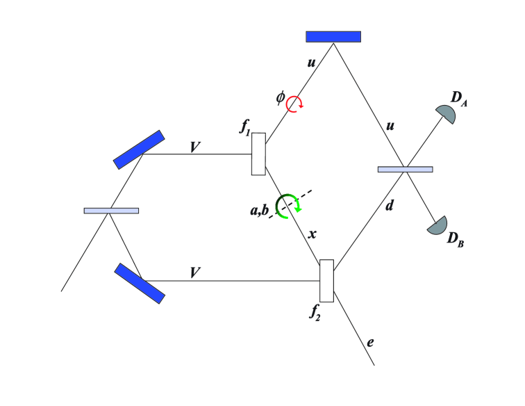
Figure 2: The Zou-Wang-Mandel interferometer mandeletal for the trans-horizon Bell-correlation experiment. Gray rectangles are 50:50 beam splitters, white rectangles are the two nonlinear parametric down-converting crystals with efficiencies $f_{1}$, $f_{2}$; blue rectangles are mirrors. A phase delay is placed on the idler beam labeled $u$, and an adjustable-angle polarization rotator is placed on the signal beam $x$ which is aligned with the second signal beam labeled $e$. Since both pump beams are blocked past the nonlinear crystals, the output state lies in the Hilbert space ${\cal H}_{u}\otimes{\cal H}_{d}\otimes{\cal H}_{e}$ of the signal and idler beams; it is monitored by the single-photon detectors $D_{A}$ and $D_{B}$.

The experiment consists of monitoring the entangled output $|\psi\rangle$ at the two single-photon detectors $D_{A}$ and $D_{B}$. For the purposes of our essentially conceptual discussion in this paper, experimental inaccuracies and noise (detector inefficiencies, dark-count rates, $\ldots$) are not relevant, and we will defer their discussion to a forthcoming paper moretocome . Thus, measurement by the perfect detector $D_{A}$ is equivalent to the projection $P_{A}=P_{\alpha}\otimes\mathbb{I}_{e}$, where $\alpha\in{\cal H}_{u}\otimes{\cal H}_{d}$ is the vector $\alpha=(|0\rangle_{u}|1\rangle_{d}+i|1\rangle_{u}|0\rangle_{d})/{\sqrt{2}}$, and a measurement (click) at $D_{B}$ is equivalent to the projection $P_{B}=P_{\beta}\otimes\mathbb{I}_{e}$, where $\beta=(|1\rangle_{u}|0\rangle_{d}+i|0\rangle_{u}|1\rangle_{d})/{\sqrt{2}}$. Calculation [using $p_{A,\;B}={\rm Tr}(P_{A,\;B}|\psi\rangle\langle\psi|)=\|P_{A,\;B}|\psi\rangle\|^{2}$] shows that the probabilities $p_{A}$ and $p_{B}$ of clicks at detectors $D_{A}$ and $D_{B}$, respectively, are given by

$$p_{A} = \frac{|V|^{2}}{2\,N^{2}}\left[\,|f_{1}|^{2}+|f_{2}|^{2}\,+\,2\,\Re\,(\,i\overline{f_{1}}f_{2}\bar{a}e^{-i\phi}\,)\,\right]\;,$$

$$p_{B} = \frac{|V|^{2}}{2\,N^{2}}\left[\,|f_{1}|^{2}+|f_{2}|^{2}\,-\,2\,\Re\,(\,i\overline{f_{1}}f_{2}\bar{a}e^{-i\phi}\,)\,\right]\;.$$ (6)

The important feature in Eqs. (6) is the interference term in brackets following the real-part sign $\Re$. Notice that the interference is oscillatory in the controlled phase delay $\phi$ and depends sensitively on the polarization angles $(a,b)$.

But how does the interference depend on the evolution of the probe beam $e$ which escapes to infinity? Let $\rho_{ud}\equiv{\rm Tr}_{e}|\psi\rangle\langle\psi|$ be the output state projected on the “laboratory” Hilbert space ${\cal H}_{u}\otimes{\cal H}_{d}$. It is straightforward to show that the detection probabilities $p_{A,\;B}$ can be alternatively computed via the expressions $p_{A,\;B}={\rm Tr}_{ud}(P_{\alpha,\;\beta}\,\rho_{ud})$. This result is, of course, valid much more generally: the expectation value of any observable $O=O_{ud}\otimes\mathbb{I}_{e}$ (i.e. one local to the Hilbert space ${\cal H}_{u}\otimes{\cal H}_{d}$) depends only on the reduced state projected on ${\cal H}_{u}\otimes{\cal H}_{d}\;$:

$${\rm Tr}\,[\,(O_{ud}\otimes\mathbb{I}_{e})\,|\psi\rangle\langle\psi|\,]={\rm Tr}_{ud}\,[\,O_{ud}\,{\rm Tr}_{e}|\psi\rangle\langle\psi|\,]\;.$$ (7)

Now suppose that the output state $|\psi\rangle$ undergoes a local quantum evolution (local in the sense that ${\cal E}={\cal E}_{ud}\otimes{\cal E}_{e}$)

$${\cal E}={\cal E}_{ud}\otimes{\cal E}_{e}\;:\;|\psi\rangle\langle\psi|\mapsto({\boldsymbol{1}}_{ud}\otimes{\cal E}_{e})(|\psi\rangle\langle\psi|)\;,$$ (8)

where ${\cal E}_{e}$ is an arbitrary, completely-positive, linear quantum map on ${\cal H}_{e}$-states which is probability preserving, with Kraus representation:

$${\cal E}_{e}:\rho\mapsto\sum_{j}E_{j}\rho{E_{j}}^{\dagger}\;,\;\;\;\;\;\sum_{j}{E_{j}}^{\dagger}E_{j}=\mathbb{I}_{e}\;,$$ (9)

where $E_{j}$ are otherwise arbitrary linear operators on ${\cal H}_{e}$. For any state $\rho$ on ${\cal H}$ [including the output state $\rho=|\psi\rangle\langle\psi|$ of Eq. (4)], by expanding $\rho$ in the form $\rho=\sum_{\mu}c_{\mu}\,{\rho_{ud}}^{(\mu)}\otimes{\sigma_{e}}^{(\mu)}$, $c_{\mu}\in\mathbb{R}$, it is straightforward to prove the identity

$${\rm Tr}_{e}\,[\,({\boldsymbol{1}}_{ud}\otimes{\cal E}_{e})\rho\,]={\rm Tr}_{e}\rho$$ (10)

for any linear map ${\cal E}_{e}$ of the form Eq. (9). In view of Eq. (7), Eq. (10) is the expression of causality (no-signaling; compare Eq. (15) below): As long as the evolution of the probe beam $e$ remains linear and probability-conserving, the interference pattern of the laboratory beams does not depend on what happens to $e$. The detection probabilities $p_{A}$ and $p_{B}$ are given by Eqs. (6) whether $e$ evolves unitarily, is absorbed in a beam block, or otherwise gets entangled with the rest of the universe.

By contrast, suppose that the beam $e$ undergoes a nonlinear, probability-conserving evolution. As an example, consider the evolution proposed in HM for evaporating black holes, whose action on any state $\rho\in{\cal H}$ is given by (see Sect. 5 below for a detailed discussion of this map class)

$${\cal E}\;:\;\rho\longmapsto\frac{{\boldsymbol{1}}_{ud}\otimes{\cal T}_{e}\;(\rho)}{{\rm Tr}[{\boldsymbol{1}}_{ud}\otimes{\cal T}_{e}\;(\rho)]}\;,$$ (11)

where ${\cal T}_{e}$ denotes the linear transformation (not a quantum map) ${\cal T}_{e}:\rho_{e}\mapsto T_{e}\rho_{e}{T_{e}}^{\dagger}$ on states $\rho_{e}$ of ${\cal H}_{e}$, and $T_{e}:{\cal H}_{e}\rightarrow{\cal H}_{e}$ is an arbitrary nonsingular linear transformation. For simplicity, let us choose $T_{e}$ in the form

$$T_{e}=\begin{pmatrix}1&0&0\cr 0&1&0\cr 0&-1&1\end{pmatrix}$$ (12)

in the $\{|0\rangle_{e},\;|1\rangle_{e},\;|-1\rangle_{e}\}$ basis of ${\cal H}_{e}$. After the incoming state $\rho=|\psi\rangle\langle\psi|$ is transformed into ${\rho}^{\ast}\equiv{\cal E}(\rho)$ according to the nonlinear evolution ${\cal E}$ given by Eqs. (11)–(12), the probabilities of detection at the local detectors can be re-calculated using the equations ${p^{\ast}}_{A,\;B}={\rm Tr}(P_{A,\;B}\,{\rho^{\ast}})$. The result for the interference signal $p_{A}-p_{B}$ is:

$${p^{\ast}}_{A}-{p^{\ast}}_{B}=\frac{2\,|V|^{2}}{{N^{\ast}}^{2}}\;\Re\left[\,i\overline{f_{1}}f_{2}\,(\bar{a}-\bar{b})\,e^{-i\phi}\,\right]\;,$$ (13)

where ${N^{\ast}}^{2}=1+|V|^{2}[\,|f_{2}|^{2}+|f_{1}|^{2}(|a-b|^{2}+|b|^{2})\,]$ is the new normalization factor. Observing a signal like Eq. (13) would represent a clean detection of the nonlinear map $\cal E$ [Eqs. (11)–(12)] by our interferometer, since, e.g., the new null and maximum of the interference with respect to the polarization-rotator angle $\theta\equiv\arctan|b/a|$ are both shifted by $45^{\circ}$ compared to Eqs. (6). In general, the interference signal $p_{A}-p_{B}$ as a function of $\phi$ and $\theta$, the fundamental observable in our proposed experiment, constitutes a rich 2D data set sensitive to almost any nonlinear evolution map affecting the probe beam $e$.

It is important to note that quantum evolution in the presence of signaling maps is incompatible with standard Cauchy evolution (in globally hyperbolic spacetimes, or within the domain of dependence of a partial Cauchy surface when global hyperbolicity fails). In fact, the phenomenon of signaling is equivalent to the well-known ambiguity that arises when one attempts to carry out time evolution from one partial Cauchy surface (i.e. a spacelike surface no causal curve intersects more than once) to another using the usual existence and uniqueness properties of the standard Cauchy problem Jacobson . Instead, one makes consistent predictions in the presence of signaling based on principles similar to the concept of “self-consistency” which provides for consistent predictions in the presence of closed timelike curves CTC . More specifically, the principle of self consistency implies the following algorithm for the consistent evolution of distributed quantum states in the presence of signaling maps: Suppose $P_{B}$ is a spacetime point where nonlinear (signaling) quantum evolution takes place, $AB$ is an entangled system whose wavefunction is localized around worldlines of $A$ and $B$, and the worldline of $B$ passes through the point $P_{B}$. Then, for self consistency, the effect of the nonlinear evolution at $P_{B}$ must extend everywhere in spacetime outside the past null cone of $P_{B}$. In predicting the evolution of the joint quantum state of $AB$, one would use the standard unitary evolution from one partial Cauchy surface to the next, and, as soon as there exists at least one partial Cauchy surface passing through $A$ and $P_{B}$ [i.e. as soon as $A$ enters the complement of $I^{-}(P_{B})$, the chronological past of $P_{B}$], apply the nonlinear evolution map to the entire state of $AB$. Of course this leads to a “teleological” influence of $P_{B}$ on the entire state, but this property is the characteristic feature of signaling maps, and it is also because of this feature that signaling maps can be used to transmit information acausally.

To apply the evolution principle discussed above to the problem corresponding to our trans-horizon Bell-correlation experiment, let $A\equiv\{u,d\}$ and $B\equiv\{e\}$ for the output state Eq. (4) as the probe beam $e$ is directed into the event horizon of a black hole. Suppose the evaporation of the hole leads to a quantum map ${\cal E}_{AB}$ with a signaling nonlinear component. Would the nonlinearity cause a detectable shift in the interference patterns of $u$ and $d$? As discussed in the above paragraph, and in accordance with standard quantum field theory, the evolution of $|\psi\rangle$ is described by ${\cal E}_{AB}$ when and only when the subsystems $A$ and $B$ are contained in a partial Cauchy surface $\Sigma_{AB}$. The blue diagram in Fig. 1 depicts such a surface $\Sigma_{AB}$ for the causal geometry of the proposed experiment. If the ultimate causal structure of the evaporating quantum black hole remains the same as given by the classical metric (Fig. 1), the singularity is a final boundary, $e$ will propagate unitarily before it disappears into the singularity, and no signal will be produced (effectively unitary ${\cal E}_{AB}$). If, on the other hand, $e$ re-emerges as Hawking radiation following evaporation [i.e. if the singularity is effectively a part of $H^{+}(\Sigma)$ in the quantum spacetime], then a detectable signal will result. Conversely, the likely null outcome of the experiment can be used to place precise upper limits on the strength of any signaling nonlinear component in the effective quantum map ${\cal E}_{AB}$ of evaporating black holes (see Sect. 6 below for more discussion on this and other feasibility questions for our proposed experiment).

4. General theory of nonlinear quantum evolution maps

If black-hole evaporation compels us to treat linearity as a property to be tested by experiment rather than as a universal axiom of quantum mechanics, what properties must hold for the most general class of quantum maps governing quantum evolution everywhere? We now turn briefly to the mathematical description of this generalized class of maps. Full details will be found in the forthcoming moretocome .

A black-hole event horizon divides spacetime naturally into two distinct regions: the external, asymptotically-flat region, $A$, and the interior region beyond the event horizon, $B$, where the causal future of $B$ does not intersect $A$. The same causal separation is natural for the more general problem where $B$ represents a distant region with a naked singularity or other extreme structure (e.g. beyond our cosmological event horizon), and $A$ represents the local spacetime neighborhood. Consider now a general quantum evolution map, defined as a map from the space of all states (density matrices) of the joint Hilbert space of $A$ and $B$ (simply $AB$) into the (linear) space of symmetric operators on the same Hilbert space. There are four key properties such an evolution map may satisfy:

• Locality: The action of the map at $A$ does not depend on the state of the system as seen at $B$, and vice versa; i.e., the form of the map’s action in one region does not depend on what the state of the system is in the other region.

• Probability conservation: The evolution sends density matrices of unit trace (normalized with unit probability) to density matrices of unit trace.

• Causality (no-signaling condition): The evolution map cannot be used to signal between $A$ and $B$ when classical communication between $A$ and $B$ is not allowed.

• Linearity: The evolution map is the restriction to states (i.e. to density matrices) of a linear transformation on the linear space of all symmetric operators in the joint Hilbert space of $AB$. (States are the positive symmetric operators of trace 1; a nonlinear subset of the space of all symmetric operators.)

Note that standard, local unitary quantum maps satisfy all four properties. We contend that while the first two conditions, namely locality and probability conservation, are indispensable for any physical evolution map, the last two conditions are not. We view locality as indispensable because relaxing it would amount to assuming communication between the physical “agents” implementing the evolution maps at $A$ and $B$, an assumption which makes acausal signaling possible even with standard unitary evolution maps, and which contradicts the presumed causal separation between the regions $A$ and $B$. Probability conservation is indispensable because its violation would be easily detectable in almost every experiment which sends physical signals from the external region $A$ into the region $B$; since no local experiment has ever detected such violations, they are ruled out on observational grounds. As for causality, we take the position that causality is a higher level notion, which should be derived as a theorem from the other more primitive laws of quantum mechanics; when it cannot be so derived, ruling out violations of causality becomes an experimental question. The same conclusion applies (with even more force) to linearity.

Given a causally separated bi-partite quantum system $AB$ with (finite-dimensional) Hilbert space ${\cal H}\equiv{\cal H}_{A}\otimes{\cal H}_{B}$, let $W({\cal H})$ be the real vector space of symmetric operators on $\cal H$, and $S({\cal H})\subset W({\cal H})$ the set of all states (positive, symmetric operators of unit trace). We propose that the set of physical quantum maps $\mathfrak{M}({\cal H})$ should consist of all smooth maps ${\cal E}_{AB}:W({\cal H})\rightarrow W({\cal H})$ which map $S({\cal H})$ into $S({\cal H})$ (conserve probability) and which satisfy an appropriate condition for locality. What form should this locality condition take for a general nonlinear map? The most general definition of locality for a linear bi-partite quantum map ${\cal E}_{AB}$ stipulates

$${\cal E}_{AB}={\rm Tr}_{RS}\,\left({\cal E}_{AR}\otimes{\cal E}_{BS}\right)\;,$$ (14)

where $R$ and $S$ are auxiliary systems co-located with $A$ and $B$, respectively, the joint system $RS$ is allowed to have prior-established entanglement (see Eqs. (15)–(18) in preskill ), and ${\cal E}_{AR}$, ${\cal E}_{BS}$ are arbitrary linear (positive and complete) quantum maps acting on the Hilbert spaces ${\cal H}_{AR}$ and ${\cal H}_{BS}$, respectively. The condition Eq. (14) is equivalent to the statement

$${\cal E}_{AB}=\sum_{\alpha}d_{\alpha}\;{\cal E}_{A\alpha}\otimes{\cal E}_{B\alpha}\;,$$ (15)

where the coefficients $d_{\alpha}$ are real numbers ($\sum_{\alpha}d_{\alpha}=1$), and ${\cal E}_{A\alpha}$ and ${\cal E}_{B\alpha}$ are linear quantum evolution maps on ${\cal H}_{A}$ and ${\cal H}_{B}$, respectively. For nonlinear maps, however, the tensor product operation is not well defined, and has no canonical generalization. Consequently, for a general (possibly nonlinear) map we adopt the more stringent (restrictive) locality condition

$${\cal E}_{AB}(\rho\otimes\sigma)={\cal E}_{A}(\rho)\otimes{\cal E}_{B}(\sigma)\;$$ (16)

for all $\rho\in S({\cal H}_{A})$ and $\sigma\in S({\cal H}_{B})$, where ${\cal E}_{A}$ and ${\cal E}_{B}$ are fixed quantum maps in $\mathfrak{M}({\cal H}_{A})$ and $\mathfrak{M}({\cal H}_{B})$ (called the local components of ${\cal E}_{AB}$) that depend only on ${\cal E}_{AB}$. When ${\cal E}_{AB}$ is a linear map, the locality condition Eq. (16) implies that ${\cal E}_{AB}$ must be in the form of a tensor product of linear maps ${\cal E}_{AB}={\cal E}_{A}\otimes{\cal E}_{B}$, where the linear maps ${\cal E}_{A}$ and ${\cal E}_{B}$ are the local components of ${\cal E}_{AB}$. Clearly, all linear maps local according to Eq. (16) are local according to the definition Eqs. (14)–(15), but not vice versa.

The condition for a map ${\cal E}_{AB}\in\mathfrak{M}$ to be signaling (non-causal) is precisely that for some $\rho_{AB}\in S({\cal H})$

$${\rm Tr}_{B}\,[\,{\cal E}_{AB}(\rho_{AB})\,]\neq{\cal E}_{A}\,[\,{\rm Tr}_{B}(\rho_{AB})\,]\;,$$ (17)

where ${\cal E}_{A}$ is the local $A$-component of ${\cal E}_{AB}$. It is easy to prove using Eq. (16) [or, more generally, Eq. (15)] that all local linear ${\cal E}_{AB}$ are causal [non-signaling; cf. Eq. (10)]: Consider any decomposition $\rho_{AB}=\sum_{i}\,c_{i}\,\rho_{Ai}\otimes\sigma_{Bi}$, where $\rho_{Ai}$ and $\sigma_{Bi}$ are normalized states. Since any local linear ${\cal E}_{AB}$ is of the form ${\cal E}_{AB}={\cal E}_{A}\otimes{\cal E}_{B}$,

$${\rm Tr}_{B}\,[\,{\cal E}_{AB}(\rho_{AB})\,] = \sum_{i}\,c_{i}\,{\rm Tr}_{B}[{\cal E}_{AB}(\rho_{Ai}\otimes\sigma_{Bi})]$$ (18)

$$= \sum_{i}\,c_{i}\,{\rm Tr}_{B}[{\cal E}_{A}(\rho_{Ai})\otimes{\cal E}_{B}(\sigma_{Bi})]=\sum_{i}\,c_{i}\,{\cal E}_{A}(\rho_{Ai})$$

$$= {\cal E}_{A}\left(\sum_{i}\,c_{i}\,\rho_{Ai}\right)={\cal E}_{A}\,[\,{\rm Tr}_{B}(\rho_{AB})\,]\;.$$

Note also that locality [Eq. (16)] explains why phase-coherent entanglement of $AB$ is essential to detect any non-causal influence of ${\cal E}_{AB}$ at $A$ when, for example, $B$ is inside the event horizon and $A$ is in the exterior region of a black hole: Any system (e.g., starlight) entangled with the external world will give rise to a decohered input state having the product form $\rho_{AB}=\rho_{A}\otimes\sigma_{B}$, and evolution of such product states cannot satisfy the signaling condition Eq. (17) because of the locality constraint Eq. (16). Experiments must carefully preserve phase-coherence of entanglement (as proposed in Fig. 2) to be able to detect signaling. We will now give a more detailed explanation of this point.

A significant component of our main argument, namely, a push for performing the trans-horizon Bell-correlation experiment, is that nonlinear maps of the kind this experiment is sensitive to would not have any observable effects that would have been visible in other experiments. There are, naturally, many other systems, such as stars, that produce multi-partite entangled quantum states, where part of the system (in the case of a star, the emitted light) might travel to distant regions which may possibly involve nonlinear quantum evolution maps. In order to make the argument that nonlinear quantum mechanics “at large distances” is not already ruled out by existing experiments, we need to show why such states are not effective probes for the putative nonlinearities. The crucial property of entangled states produced by systems such as stars is that they have completely random relative phases. For example, assuming, for conceptual simplicity, two-dimensional Hilbert spaces ${\cal H}_{A}$, corresponding to the emitters, and ${\cal H}_{B}$, corresponding to the emitted light, the “starlight states” are of the form:

$$|\psi\rangle=\frac{1}{2}(|00\rangle+|01\rangle e^{i\phi_{1}}+|10\rangle e^{i\phi_{2}}+|11\rangle e^{i\phi_{3}})$$ (19)

where $|00\rangle$ etc. denotes $|0\rangle_{A}\otimes|0\rangle_{B}$ etc. Therefore, effectively, the input state (in ${\cal H}_{A}\otimes{\cal H}_{B}$) is given by the average:

$$\frac{1}{(2\pi)^{3}}\int_{0}^{2\pi}\int_{0}^{2\pi}\int_{0}^{2\pi}d\phi_{1}\,d\phi_{2}\,d\phi_{3}\;|\psi\rangle\langle\psi|=\frac{1}{4}\;{\boldsymbol{1}}_{A}\otimes{\boldsymbol{1}}_{B}\;.$$ (20)

An alternative derivation of the same conclusion Eq. (20) may be given as follows: The systems $A$ (emitters) and $B$ (starlight) are entangled with a third system, a reservoir representing the “environment.” In the larger Hilbert space of the full system including the environment, starlight states correspond to states of the form

$$|\psi\rangle=\frac{1}{2}(|00\rangle|e_{0}\rangle+|01\rangle|e_{1}\rangle+|10\rangle|e_{2}\rangle+|11\rangle|e_{3}\rangle)$$ (21)

where the $|e_{i}\rangle$ denote orthonormal states of the environment. In other words, the “probe beam” is decoherent with the environment. However, it’s not just the probe beam which is entangled with the environment, but the entire state of the “apparatus,” which in this example corresponds to not only the starlight ($B$), but also whatever other system (the sources $A$) in the star that is producing the starlight. (In our proposed Bell-correlation experiment of Fig. 2, the apparatus $AB$ is a three-partite system; so this bi-partite example is a bit simplified, but the main conclusion remains the same). Again, when traced over the environment, the input state becomes

$${\rm Tr}_{\rm Env}\;|\psi\rangle\langle\psi|=\frac{1}{4}\;{\boldsymbol{1}}_{A}\otimes{\boldsymbol{1}}_{B}\;;$$ (22)

which is as before the maximally mixed state (a maximally mixed state is always in product form).

In the above very simple example, we assumed that there is no preferred orthonormal basis state in ${\cal H}_{A}\otimes{\cal H}_{B}$ for a quantum state $|\psi\rangle$ produced by a random process. In general, there may exist “superselection sectors” determined by conserved quantities (such as energy or charge), and basis states in different sectors (e.g. at different energy levels) may have different weights. For example, a thermal state has this property. For “thermal” starlight, the system state would have to be, instead of Eq. (21), an input state $|\psi\rangle$ which when traced over the environment takes the form

$${\rm Tr}_{\rm Env}\;|\psi\rangle\langle\psi|=\frac{1}{Z}\sum_{j,\;k}e^{-\beta({E}_{jA}+{E}_{kB})}\;\frac{{\boldsymbol{1}}_{jA}}{d_{jA}}\otimes\frac{{\boldsymbol{1}}_{kB}}{d_{kB}}\;$$ (23)

where $Z\equiv\sum_{j,\,k}e^{-\beta({E}_{jA}+{E}_{kB})}$, and ${\boldsymbol{1}}_{jA}$, ${\boldsymbol{1}}_{kB}$ denote the identity operators in the respective energy eigenspaces (of dimensions $d_{jA}$ and $d_{kB}$, and eigenvalues ${E}_{jA}$ and ${E}_{kB}$) of ${\cal H}_{A}$ and ${\cal H}_{B}$, respectively. In this more general case the input is not a maximally mixed state, but it is still a product state, e.g. in Eq. (23) the product of two separate thermal states for $A$ and for $B$.

To recap: the key observation is that entangled states produced by random processes have random relative phases, and when parts of these states fall into a region with a nonlinear evolution map, effectively the input to the map is reduced to a product state, whose evolution is guaranteed to be causal by the locality condition Eq. (16). Put differently, a distant region with a nonlinear evolution map might cause random interference fringes throughout the observable universe to shift; but random fringes disappear when averaged over the varying relative phases, therefore any shift in these fringes also vanishes when averaged, leaving no observable effect of the map in the external universe. In order to see any effect of the nonlinear maps possibly lurking in distant extreme regions of spacetime, it is necessary to design an experiment which can send probe states out to infinity that are entangled with laboratory states with known, coherently controlled phases.

If we denote the class of (local, completely positive) linear maps by $\mathfrak{L}\subset\mathfrak{M}({\cal H})$, the complement (nonlinear maps) by $\mathfrak{NL}=\mathfrak{M}\setminus\mathfrak{L}$, and the class of signaling maps by $\mathfrak{S}$, we have just shown that $\mathfrak{S}\cap\mathfrak{L}=\{\}$. In moretocome , we will give a complete algebraic characterization of nonlinear maps satisfying the locality condition Eq. (16), and show that it is straightforward to produce both signaling and non-signaling examples for maps in $\mathfrak{NL}$ gisinetal ; that is, $\mathfrak{S}$ is a non-empty proper subset of $\mathfrak{NL}$. The evolution map $\cal E$ defined by Eqs. (11)–(12) is one example of a class of local nonlinear maps—proposed by Horowitz and Maldacena in HM to describe quantum evolution through evaporating black holes—that are signaling (i.e., belong to $\mathfrak{S}$). A detailed analysis of the Horowitz-Maldacena class of maps, along with a discussion of the motivation for them, is what we turn to in the next Section.

5. Nonlinear quantum maps associated with evaporating black holes

We begin with a brief review of the final-state boundary condition for evaporating black holes as proposed in HM and further elucidated in GP . In the semiclassical approximation, the overall Hilbert space for the evaporation process can be treated as a decomposition

$${\cal H}={\cal H}_{M}\otimes{\cal H}_{F}={\cal H}_{M}\otimes{\cal H}_{\rm in}\otimes{\cal H}_{\rm out}\;,$$ (24)

where ${\cal H}_{M}$ denotes the Hilbert space of the quantum field that constitutes the collapsing body, and ${\cal H}_{F}$ is the Hilbert space in which the quantum-field fluctuations around the background spacetime determined by the ${\cal H}_{M}$ quantum state live. The separation of ${\cal H}$ into ${\cal H}_{M}$ and ${\cal H}_{F}$ reflects the semiclassical nature of the treatment in a fundamental way. Moreover, the fluctuation Hilbert space ${\cal H}_{F}$ can be further decomposed as ${\cal H}_{F}={\cal H}_{\rm in}\otimes{\cal H}_{\rm out}$, where ${\cal H}_{\rm in}$ and ${\cal H}_{\rm out}$ denote the Hilbert spaces of fluctuation modes confined inside and outside the event horizon, respectively. Before evaporation, the quantum state $|\;\rangle\in{\cal H}$ of the complete system can be written as a product

$$|\;\rangle=|\psi_{0}\rangle_{M}\otimes|0_{U}\rangle\;,$$ (25)

where $|\psi_{0}\rangle_{M}\in{\cal H}_{M}$ is the initial wave function of the collapsing matter, and the Unruh vacuum $|0_{U}\rangle\in{\cal H}_{F}={\cal H}_{\rm in}\otimes{\cal H}_{\rm out}$ is the maximally entangled state

$$|0_{U}\rangle=\frac{1}{\sqrt{N}}\sum_{k=1}^{N}|k_{\rm in}\rangle\otimes|k_{\rm out}\rangle\;.$$ (26)

Here $N$ is the common dimension (the number of degrees of freedom necessary to completely describe the internal state of the black hole) of all three Hilbert spaces ${\cal H}_{M}$, ${\cal H}_{\rm in}$, and ${\cal H}_{\rm out}$, and $\{|k_{\rm in}\rangle\}$ and $\{|k_{\rm out}\rangle\}$, $k=1,2,\cdots,N$, are fixed orthonormal bases for ${\cal H}_{\rm in}$ and ${\cal H}_{\rm out}$, respectively. After the hole evaporates completely, the “final” Hilbert space is simply ${\cal H}_{\rm out}$, and, as we argued in Sec. 1 above, the usual semiclassical arguments inevitably imply a mixed state $\rho_{\rm out}$ as the endpoint of complete evaporation (see Fig. 1 and the associated discussion), revealing that the transition $|\psi_{0}\rangle_{M}\mapsto\rho_{\rm out}$ is manifestly non-unitary.

The Horowitz-Maldacena proposal (HM) imposes a boundary condition on the final quantum state at the black-hole singularity by demanding that it be equal to

$$|\Phi\rangle\equiv U^{\dagger}\left[\frac{1}{\sqrt{N}}\sum_{j=1}^{N}|j_{M}\rangle\otimes|j_{\rm in}\rangle\right]\in{\cal H}_{M}\otimes{\cal H}_{\rm in}$$ (27)

where $\{|j_{M}\rangle\}$ is an orthonormal basis for ${\cal H}_{M}$, and $U:{\cal H}_{M}\otimes{\cal H}_{\rm in}\rightarrow{\cal H}_{M}\otimes{\cal H}_{\rm in}$ is a unitary transformation. More precisely, HM states the following:

There exists a unitary map $U:{\cal H}_{M}\otimes{\cal H}_{\rm in}\rightarrow{\cal H}_{M}\otimes{\cal H}_{\rm in}$ such that with $|\Phi\rangle\in{\cal H}$ defined as in Eq. (27), the state $|\;\rangle$ [Eqs. (25)–(26)] evolves after complete evaporation as

$$|\;\rangle\longmapsto\alpha\,P_{|\Phi\rangle\otimes{\cal H}_{\rm out}}\;|\;\rangle\;,$$ (28)

where $\alpha\in\mbox{\bbold R}$ is a renormalization constant, and $P_{|\Phi\rangle\otimes{\cal H}_{\rm out}}$ denotes the projection onto the linear subspace $|\Phi\rangle\otimes{\cal H}_{\rm out}\equiv\{|\Phi\rangle\otimes|v\rangle:\;|v\rangle\in{\cal H}_{\rm out}\}$ of $\cal H$.

The unitary operator $U$ describes the non-local evolution of the black-hole quantum state near the singularity, as well as its evolution in the semiclassical regime before the singularity; one would expect a full quantum theory of gravity to be able to completely specify this operator. To restore unitarity to the transition map ${\cal H}_{M}\rightarrow{\cal H}_{\rm out}$, Horowitz and Maldacena HM further demand that $U$ be in the form of a product corresponding to the absence of entangling interactions between ${\cal H}_{M}$ and ${\cal H}_{\rm in}$:

$$U=S_{1}\otimes S_{2}\;,$$ (29)

where $S_{1}:{\cal H}_{M}\rightarrow{\cal H}_{M}$ and $S_{2}:{\cal H}_{\rm in}\rightarrow{\cal H}_{\rm in}$ are unitary maps. To find the effective evolution map ${\cal H}_{M}\rightarrow{\cal H}_{\rm out}$ resulting from HM and the assumption Eq. (29), start from the equality

$$\alpha\,P_{|\Phi\rangle\otimes{\cal H}_{\rm out}}\;(\,|\psi_{0}\rangle_{M}\otimes|0_{U}\rangle\,)=|\Phi\rangle\otimes|X_{\rm out}\rangle\;,$$ (30)

where $|X_{\rm out}\rangle$ is the state in ${\cal H}_{\rm out}$ into which the initial state $|\psi_{0}\rangle_{M}$ evolves after the evaporation. Contracting both sides of Eq. (30) with $\langle\Phi|$ substituted from Eq. (27)

$$|X_{\rm out}\rangle = \frac{\alpha}{N}\sum_{j=1}^{N}\langle j_{M}|\otimes\langle j_{\rm in}|(S_{1}\otimes S_{2})|\psi_{0}\rangle_{M}\otimes\sum_{k=1}^{N}|k_{\rm in}\rangle\otimes|k_{\rm out}\rangle$$ (31)

$$= \frac{\alpha}{N}\sum_{j=1}^{N}\sum_{k=1}^{N}\langle j_{M}|S_{1}|\psi_{0}\rangle_{M}\,\langle j_{\rm in}|S_{2}|k_{\rm in}\rangle\;|k_{\rm out}\rangle\;.$$

In terms of the basis components $X_{{\rm out}\;j}\equiv\langle j_{\rm out}|X_{\rm out}\rangle$, $\psi_{0\;k}\equiv\langle k_{M}|\psi_{0}\rangle_{M}$, $S_{1\;jk}\equiv\langle j_{M}|S_{1}|k_{M}\rangle$, and $S_{2\;jk}\equiv\langle j_{\rm in}|S_{2}|k_{\rm in}\rangle$, Eq. (31) can be rewritten in the matrix form

$$X_{{\rm out}\;k}=\frac{\alpha}{N}\sum_{l=1}^{N}({S_{2}}^{T}S_{1})_{\,kl}\;\psi_{0\;l}\;\;,$$ (32)

where $S^{T}$ denotes matrix transpose of $S$. Since the transpose of a unitary matrix is still unitary, Eq. (32) shows that (i) the renormalization constant $\alpha=N$, and (ii) the transformation $|\psi_{0}\rangle_{M}\mapsto|X_{\rm out}\rangle$ is unitary.

However, as pointed out by Gottesman and Preskill GP , entangling interactions between ${\cal H}_{M}$ and ${\cal H}_{\rm in}$ are unavoidable in any reasonably generic gravitational collapse scenario. Consequently, we cannot expect the unitary operator $U$ to have the product form Eq. (29) in general. For a general unitary map $U:{\cal H}_{M}\otimes{\cal H}_{\rm in}\rightarrow{\cal H}_{M}\otimes{\cal H}_{\rm in}$, the vector $|\Phi\rangle$ defined by Eq. (27) is an arbitrary element in ${\cal H}_{M}\otimes{\cal H}_{\rm in}$, and Eq. (31) leads to the more general linear expression

$$X_{{\rm out}\;k}={\alpha}\sum_{l=1}^{N}T_{\,kl}\;\psi_{0\;l}\;\;$$ (33)

instead of Eq. (32). Here $T$ denotes the matrix

$$T_{kl}\equiv\frac{1}{\sqrt{N}}\langle\,\Phi\;|l_{M}\rangle\!\otimes\!|k_{\rm in}\rangle$$ (34)

which is unconstrained except for $\sum_{kl}|T_{kl}|^{2}=1/N$. Only when $U$ has the product form Eq. (29) $T$ equals ($1/N$ times) a unitary matrix [Eq. (32)]. Note that the constant $\alpha$ is to be determined from the condition that $|X_{\rm out}\rangle$ remains normalized. After this renormalization, we can express the transformation ${\cal H}_{M}\rightarrow{\cal H}_{\rm out}$ described by Eq. (33) more succinctly in the form

$$X_{{\rm out}\;k}=\frac{1}{(\,\sum_{i}|\!\sum_{j}T_{\,ij}\;\psi_{0\;j}|^{2}\,)^{\frac{1}{2}}}\sum_{l=1}^{N}T_{\,kl}\;\psi_{0\;l}\;\;$$ (35)

where now $T$ is a completely unconstrained, arbitrary matrix ftnote3 . While it maps pure states to pure states, the transformation ${\cal H}_{M}\rightarrow{\cal H}_{\rm out}$ specified by Eq. (35) is not only nonunitary, but it is in fact nonlinear; linearity is recovered (along with unitarity) only when $T$ is proportional to a unitary matrix.

In the preceding Sects. 1–4, we argued that nonlinear quantum evolution inside an evaporating black hole might have observable consequences outside the event horizon when an entangled system (whose coherence is carefully monitored) partially falls into the hole. In Sect. 3 we proposed a specific experiment that should be able to detect the presence of such signaling nonlinear maps via terrestrial quantum interferometry. We will now show that the HM-class of nonlinear maps defined in Eq. (35) in fact belong to this signaling class quite generally. Therefore, the HM boundary-condition proposal can in principle be tested by terrestrial experiments.

Let us assume a causal configuration as depicted in Fig. 1, where a bipartite system $AB$ evolves to send its $B$-half into a black-hole event horizon along a null geodesic, while the $A$-half remains coherently monitored outside the horizon. We can then further decompose the “collapsing” Hilbert space ${\cal H}_{M}$ in the form ${\cal H}_{M}={\cal H}_{A}\otimes{\cal H}_{B}$, where ${\cal H}_{B}$ now corresponds to all matter that falls into the black hole, including the “probe beam” $e$ of our trans-horizon Bell-correlation experiment (cf. Fig. 2 and the discussion following it in Sect. 3), and ${\cal H}_{A}$ corresponds to all matter that remains outside the horizon, including the interferometer beams which are monitored in the laboratory. We also identify the outgoing Hilbert space ${\cal H}_{\rm out}$ with ${\cal H}_{M}$, which amounts to specifying a unitary map $U_{M}:{\cal H}_{M}\rightarrow{\cal H}_{\rm out}$ connecting orthonormal basis sets in the two spaces. With this identification, the “evaporation” map ${\cal H}_{M}\rightarrow{\cal H}_{\rm out}$ can be treated simply as a map sending ${\cal H}_{M}$ onto ${\cal H}_{M}$. Reinterpreted thus, the action of a general quantum map in the class defined by Eq. (35) can be written as

$$\rho_{AB}\longmapsto\frac{T\,\rho_{AB}\,T^{\dagger}}{{\rm Tr}(T\,\rho_{AB}\,T^{\dagger})}\;$$ (36)

on any state $\rho_{AB}$ in ${\cal H}_{M}={\cal H}_{A}\otimes{\cal H}_{B}$, where $T:{\cal H}_{A}\otimes{\cal H}_{B}\rightarrow{\cal H}_{A}\otimes{\cal H}_{B}$ is a (nonsingular) general linear transformation ftnote3 . To satisfy the locality condition as formulated in Eq. (16), the map $T$ must have the product form

$$T=T_{A}\otimes T_{B}\;,$$ (37)

where $T_{A}:{\cal H}_{A}\rightarrow{\cal H}_{A}$ and $T_{B}:{\cal H}_{B}\rightarrow{\cal H}_{B}$ are general linear maps. Since subsystem $A$ remains outside the event horizon, the evolution map $T_{A}$ must remain unitary, and we can assume (for simplicity and without loss of generality) that $T_{A}=\mathbb{I}_{A}$. Then the quantum evolution map Eq. (36) acting on the Hilbert space ${\cal H}_{M}={\cal H}_{A}\otimes{\cal H}_{B}$ takes the more transparent form

$${\cal E}_{AB}\;:\;\rho_{AB}\longmapsto\frac{{\boldsymbol{1}}_{A}\otimes{\cal T}_{B}\;(\rho_{AB})}{{\rm Tr}[{\boldsymbol{1}}_{A}\otimes{\cal T}_{B}\;(\rho_{AB})]}\;,$$ (38)

where ${\boldsymbol{1}}_{A}={\cal E}_{A}$ denotes the identity map on states of ${\cal H}_{A}$, and ${\cal T}_{B}$ denotes the linear transformation (not a quantum map)

$${\cal T}_{B}\;:\;\rho_{B}\longmapsto T_{B}\,\rho_{B}\,{T_{B}}^{\dagger}\;$$ (39)

on states of ${\cal H}_{B}$. When $\rho_{AB}$ is a product state $\rho_{AB}=\rho_{A}\otimes\rho_{B}$, the action of ${\cal E}_{AB}$ has the manifestly local form

$${\cal E}_{AB}(\rho_{AB})={\cal E}_{A}(\rho_{A})\otimes{\cal E}_{B}(\rho_{B})\;,$$ (40)

where ${\cal E}_{A}={\boldsymbol{1}}_{A}$, and ${\cal E}_{B}$ is the nonlinear quantum map

$${\cal E}_{B}\;:\;\rho_{B}\longmapsto\frac{{\cal T}_{B}(\rho_{B})}{{\rm Tr}_{B}[{\cal T}_{B}(\rho_{B})]}=\frac{T_{B}\rho_{B}{T_{B}}^{\dagger}}{{\rm Tr}_{B}(T_{B}\rho_{B}{T_{B}}^{\dagger})}\;$$ (41)

mapping ${\cal H}_{B}$-states onto ${\cal H}_{B}$-states (compare Eq. (40) with Eq. (16) above in Sect. 4). By contrast, when $\rho_{AB}$ is entangled the action of ${\cal E}_{AB}$ does not have the simple product form of Eq. (40).

In Sect. 4 above, we identified the criterion for a quantum map ${\cal E}_{AB}$ to be signaling [see Eq. (17) and the associated discussion] as simply the condition that

$${\rm Tr}_{B}\,[\,{\cal E}_{AB}(\rho_{AB})\,]\neq{\cal E}_{A}\,[\,{\rm Tr}_{B}(\rho_{AB})\,]\;$$ (42)

for some (necessarily entangled) state $\rho_{AB}$. Now consider a class of entangled states $\rho_{AB}$ in the form of a convex linear combination

$$\rho_{AB}=\lambda_{1}\,\rho_{A}\otimes\rho_{B}+\lambda_{2}\,\sigma_{A}\otimes\sigma_{B}\;,$$ (43)

where $\rho_{A},\;\sigma_{A}$ , and $\rho_{B},\;\sigma_{B}$ are (normalized) states in ${\cal H}_{A}$ and ${\cal H}_{B}$, respectively, and $\lambda_{1}>0,\;\lambda_{2}>0,\;\lambda_{1}+\lambda_{2}=1$ are real coefficients. Introduce the real numbers

$$n_{1} \equiv {\rm Tr}_{B}[{\cal T}_{B}(\rho_{B})]={\rm Tr}_{B}(T_{B}\rho_{B}{T_{B}}^{\dagger})\;,$$

$$n_{2} \equiv {\rm Tr}_{B}[{\cal T}_{B}(\sigma_{B})]={\rm Tr}_{B}(T_{B}\sigma_{B}{T_{B}}^{\dagger})\;.$$ (44)

The right-hand-side of Eq. (42) is simply ${\rm Tr}_{B}(\rho_{AB})$ (recall that ${\cal E}_{A}={\boldsymbol{1}}_{A}$):

$${\cal E}_{A}\,[\,{\rm Tr}_{B}(\rho_{AB})]=\lambda_{1}\rho_{A}+\lambda_{2}\sigma_{A}\;,$$ (45)

while the left-hand-side is

$${\rm Tr}_{B}\,[\,{\cal E}_{AB}(\rho_{AB})\,]=\frac{\lambda_{1}\,n_{1}\,\rho_{A}\;+\;\lambda_{2}\,n_{2}\,\sigma_{A}}{\lambda_{1}\,n_{1}+\lambda_{2}\,n_{2}}\;.$$ (46)

But

$$\lambda_{1}\rho_{A}+\lambda_{2}\sigma_{A}\;\neq\;\frac{\lambda_{1}\,n_{1}\,\rho_{A}\;+\;\lambda_{2}\,n_{2}\,\sigma_{A}}{\lambda_{1}\,n_{1}+\lambda_{2}\,n_{2}}$$ (47)

unless at least one of the conditions: (i) $n_{1}=n_{2}$, or (ii) $\rho_{A}=\sigma_{A}$ holds. The condition (i) does not hold in general unless the linear operator $T_{B}$ is unitary (or a scalar multiple of a unitary operator), and condition (ii) does not hold in general unless $\rho_{AB}$ is a product state. Therefore the nonlinear quantum map ${\cal E}_{AB}$ defined by Eqs. (38)–(39) is in general in the signaling class. A specific example of a map in this class, and the signal that it produces in the Zou-Wang-Mandel interferometer of our proposed experiment, were described in Sect. 3 above [cf. Eqs. (11)–(13)].

6. Experimental prospects for the detection of distant nonlinearities via terrestrial probes

We have shown that the quantum maps which likely characterize quantum evolution through evaporating black holes according to the Horowitz-Maldacena HM boundary-condition proposal are a signaling class. It is clear that the HM-class of maps are in principle detectable with the apparatus of our proposed Bell-correlation experiment, namely the Zou-Wang-Mandel (ZWM) interferometer depicted in Fig. 2 [for the specific example of Eqs. (11)–(13), the detection signal is a $45^{\circ}$ shift in the detector’s interference fringes]. What are the practical prospects for actually detecting the presence of signaling nonlinear maps inside black-holes, assuming such maps do indeed exist? The set of phenomena which may impede detection efficiency in the trans-horizon Bell-correlation experiment can be naturally divided into two types according to whether they take place inside or outside the event horizon.

Inside the event horizon, the precise nature of the signal produced in the ZWM interferometer when the probe beam is sent into an evaporating hole will depend on the nature of the unitary operator $U$ characterizing the HM boundary condition, Eq. (27). If, as predicted HM ; GP , the operator $U$ involves nonlocal phases which oscillate chaotically at Planckian frequencies near the singularity, then each ZWM photon entering the hole is likely to experience a different nonlinear evolution map ${\cal E}_{AB}$, and the observed signal will be an average over such maps. Preliminary calculations show that this averaging will affect the local interference pattern back in the laboratory by erasing relative phases and thus drastically reducing fringe visibility. The ultimate result of the fluctuations is a complete erasure of the interference pattern [Eqs. (6)]. While this erasure gives rise to a qualitatively different signal than Eq. (13), the absence or reduction of interference still constitutes a strong detection signal in the ZWM setup; in other words, signal strength, i.e. the capability of the ZWM instrument to terrestrially detect nonlinear maps, is not diminished. In the ZWM interferometer, “no detection” corresponds to the presence of the specific interference pattern Eqs. (6); any deviation from this two-dimensional data set (i.e. the quantity $p_{A}-p_{B}$ as a function of the angles $\phi$ and $\theta=\arccos|a|$) would register as a detection of nonlinear quantum evolution along the probe beam, since no other physical phenomena can give rise to such deviations. This robustness of the detection signal in the presence of a rapidly fluctuating nonlinear map is a distinguishing feature of the ZWM instrument, and places it in contrast with other possible experimental designs to search for nonlinear quantum evolution at large distances. Clearly, the ZWM interferometer is not the only instrument capable of probing distant nonlinearities in quantum mechanics; any entangled system can in principle be used as such a probe. However, the second-order interference [i.e. the specific interference pattern Eqs. (6) between the $u$–$d$ beams which is maintained after tracing over the probe beam’s Hilbert space ${\cal H}_{e}$] makes the ZWM interferometer more sensitive to violations of linearity along the probe beam than other, more obvious experiments one can design. For example, when relative phases are carefully controlled, an EPR pair of polarization-entangled photons can be used as a simple detector by monitoring the polarization statistics of the local, “laboratory” photon while the other, “probe” photon escapes to infinity. Indeed, it can be shown moretocome that precisely because of the expected fluctuating geometry inside the event horizon, such a detector cannot detect HM-maps of the type Eqs. (38)–(39), in contrast with the ZWM detector which can. A detailed quantitative analysis of the interferometric response to fluctuating nonlinear maps will be given in the forthcoming paper moretocome .

Outside the event horizon, environmental decoherence of the probe beam at large distances places other fundamental limits on the visibility of any deviations from the standard “unitary” interference signal Eqs. (6) in our proposed experiment. Additional limits arise from the diffraction of the probe beam at large distances, which will let only a small fraction of the beam’s “footprint” to impact a black hole. There are also obvious difficulties with targeting specific black-hole candidates which might limit the ultimate experiment to a global search across the sky. A detailed analysis of these limits will be given in moretocome . At the very least, an easier to obtain, but perhaps less interesting, result of the experiment would be to place novel limits on possible nonlinearities nlrefs ; weinberg in the quantum evolution of the probe beam $e$ as it propagates through free space.

Acknowledgements

The research described in this paper was carried out at the Jet Propulsion Laboratory under a contract with the National Aeronautics and Space Administration (NASA), and was supported by grants from NASA and the Defense Advanced Research Projects Agency. We would like to thank our colleagues in the Quantum Computing Technologies group at JPL, in particular Jonathan Dowling and Chris Adami, for stimulating discussions.

References

- (1) J. S. Bell, Physics 1, 195 (1964).
- (2) S. Hawking, Phys. Rev. D14, 2460 (1976).
- (3) R. Haag, Commun. Math. Phys. 60, 1 (1978); N. Gisin, Phys. Lett. A143, 1 (1990); J. Polchinski, Phys. Rev. Lett. 66, 397 (1991); G. A. Goldin and G. Svetlichny, J. Math. Phys. 35, 3322 (1994); H. D. Doebner and G. A. Goldin, Phys. Rev. A54, 3764 (1996); M. Czachor, Phys. Rev. A57, 4122 (1998) and A58, 128 (1998); B. Mielnik, Phys. Lett. A289, 1 (2001).
- (4) S. Weinberg, Phys. Rev. Lett. 62(5), 485 (1989); Ann. Phys. 194, 336 (1989).
- (5) Z. Ou, L. Wang, X. Zou, L. Mandel, Phys. Rev. A41, 1597 (1990); X. Zou, L. Wang, L, Mandel, Phys. Rev. Lett. 67(3), 318 (1991); Phys Rev. A44(7), 4614 (1991).
- (6) G. T. Horowitz and J. Maldacena, hep-th/0310281.
- (7) D. Gottesman and J. Preskill, hep-th/0311269.
- (8) B. S. DeWitt, Phys. Rep. 19 C, 297 (1975); G. W. Gibbons and M. J. Perry, Phys. Rev. Lett. 36, 985 (1976); W. G. Unruh and N. Weiss, Phys. Rev. D29, 1656 (1984). See also T. Jacobson, gr-qc/9404039, gr-qc/0308048, and the references therein.
- (9) We do not agree with the arguments that evaporation non-unitarity should be necessarily detectable in low-energy experiments (see, eg., T. Banks, M. E. Peskin, and L. Susskind, Nucl. Phys. B244 , 125 (1984)) because the low-energy coupling to virtual black-hole processes such arguments rely on is exceedingly speculative.
- (10) For maps sending pure states to pure states, linearity (plus probability conservation) is equivalent to unitarity.
- (11) G. Hockney and U. Yurtsever, in preparation.
- (12) T. Jacobson, in Abstracts of Contributed Papers: 12th International Conference on General Relativity and Gravitation, (1989); and in Conceptual Problems of Quantum Gravity, ed. A. Ashtekar and J. Stachel (Birkhäuser, 1991), pp. 212-216.
- (13) J. Friedman et. al., Phys. Rev. D42, 1915 (1990).
- (14) D. Beckman, D. Gottesman, M. Nielsen, and J. Preskill, Phys. Rev. A64, 052309 (2001)].
- (15) C. Simon, V. Buz̆ek, and N. Gisin, Phys. Rev. Lett. 87, 170405 (2001); 90, 208902 (2003).
- (16) The only constraint on the linear operator entering the construction Eq. (35) or Eq. (36) is that must not have zero as an eigenvalue (e.g., projection-like operators are excluded), since with a singular this construction fails to give a well-defined quantum map.