On the stability of general relativistic geometric thin disks

Abstract

The stability of general relativistic thin disks is investigated under a general first order perturbation of the energy momentum tensor. In particular, we consider temporal, radial and azimuthal “test matter” perturbations of the quantities involved on the plane $z=0$. We study the thin disks generated by applying the “displace, cut and reflect” method, usually known as the image method, to the Schwarzschild metric in isotropic coordinates and to the Chazy-Curzon metric and the Zipoy-Voorhees metric ($\gamma$-metric) in Weyl coordinates. In the case of the isotropic Schwarzschild thin disk, where a radial pressure is present to support the gravitational attraction, the disk is stable and the perturbation favors the formation of rings. Also, we found the expected result that the thin disk models generated by the Chazy-Curzon and Zipoy-Voorhees metric with only azimuthal pressure are not stable under a general first order perturbation.

PACS: 04.40.Dg, 98.62.Hr, 04.20.Jb

I Introduction

In the last decades, analytical axially symmetric disk solutions have appeared in both Newtonian and General Relativistic formulations. In the context of General Relativity, several exact solutions were found, among them the static disks without radial pressure studied by Bonnor and Sackfield bon:sac and Morgan and Morgan mor:mor1 . Disks with radial pressure and with radial tension have been considered by Morgan and Morgan mor:mor2 and Gonzáles and Letelier gon:let1 , respectively. Also, stationary disk models including electric fields led:zof , magnetic fields let , and both electric and magnetic fields kat:bic have been studied. Self similar static disks were considered by Lynden-Bell and Pineault lyn:pin and Lemos lem . Furthermore, the superposition of black holes with static disks were analyzed by Lemos and Letelier lem:let1 ; lem:let2 ; lem:let3 and Klein kle . Bičák and Ledvinka bic:led found relativistic counter-rotating thin disks as sources of Kerr type metrics, and Bičák, Lynden-Bell and Katz bic:lyn obtained static disks as sources of known vacuum spacetimes from the Chazy-Curzon metric cha ; cur and Zipoy-Voorhees metric zip ; voo , also Bičák, Lynden-Bell and Pichon bic:lyn2 found an infinite number of new static solutions. Recently, exact solutions for thin disks with single and composite halos of matter vog:let , thin disks made of charged dust vog:let2 , thin disks made of charged perfect fluid vog:let3 , and thick disks gon:let2 were obtained. For a survey on relativistic gravitating disks, see sem .

It is well known that the formation of stellar systems lays in its stability. The study of stability, analytically or numerically, is vital to the acceptance and applicability of the different models found in the literature to describe stellar structures found in Nature. On the other hand, the study of different types of perturbations, when applied to stellar structures, usually give an insight on the formation of bars, rings or different stellar patterns. Also, a perturbation may cause the collapse of an stable object with the posterior appearance of a different kind of structure.

In Newtonian theory, perturbations have been made extensively through the years in analytical calculations and numerical experiments. An analytical treatment of the stability of thin disks can be found in Refs. bin:tre ; fri:pol and references therein. In General Relativity, the stability analysis is usually done studying the particle motion along geodesics and not perturbing the energy momentum tensor of the fluid and its conservation equations. The stability of particle motion along geodesics have been studied transforming the Rayleigh criteria of stability ray ; lan:lif into a General Relativistic formulation, see let2 and reference therein. By using this criterion, the stability of orbits around black holes surrounded by disks, rings and multipolar fields were analyzed in let2 . Also, it was employed in vog:let to test stability in the isotropic Schwarzschild thin disk, and thin disks of single and composite halos generated from the Buchdahl solution buc and Narlikar, Patwardhan and Vaidya solution nar:pat by using the displace, cut and reflect method. For the stability of circular orbits in stationary axisymmetric spacetimes see Ref. bar ; abr:pra . The stability of circular orbits of the Lemos-Letelier solution lem:let2 for the superposition of a black hole and a flat ring, as well as other aspects of this solution, are considered in detail in sem:zac ; sem:zac2 ; sem2 . Bičák, Lynden-Bell and Katz bic:lyn analyzed the stability of the Chazy-Curzon and Zipoy-Voorhees thin disks without radial pressure or tension studying their velocity curves and specific angular momentum, finding that they are not stable for highly relativistic disks. A general stability study of a relativistic fluid, with both bulk and dynamical viscosity, perturbing its energy momentum tensor was done by Seguin seg . However, he consider the coefficients of the perturbed variables as constants, i.e., local perturbations. Fact that in general is too restrictive.

The purpose of this work is to study numerically the stability of several analytical thin disk solutions in the context of General Relativity. The stability is studied performing a general first order perturbation in the temporal, radial and azimuthal components of the quantities involved in the energy momentum tensor of the fluid and analyzing the corresponding perturbed conservation equations of motion. The perturbations considered do not modified the background metric obtained from the solution of Einstein equations, i.e.they are treated as “test matter”.

The article is organized as follows. In Section II-A we present the perturbed conservation equations for the general case, when the energy momentum tensor is diagonal with the energy density and the three pressures or tensions all different from zero. Later, in Section II-B, we specialize these perturbed equations for the thin disk case where we have a distributed energy momentum tensor with support on the plane $z=0$. In Section III, we analyze the perturbed conservation equations to study the stability of the isotropic Schwarzschild thin disk, which contains radial and azimuthal pressures. In Section IV, we analyze the perturbed conservation equations to study the stability of the Chazy-Curzon and Zipoy-Voorhees thin disks with only azimuthal pressure. It is worth to mention that different Chazy-Curzon and Zipoy-Voorhees thin disks models with radial tensions or pressures can be built by using a different set of coordinates, but these models do not usually satisfy all the physical requirements, see gon:let1 . Finally, in Section V, we summarize and discuss the presented results.

II Perturbed equations

II.1 General case

Let us consider the general static, axially symmetric metric

$$ds^{2}=-e^{2\Psi_{1}}dt^{2}+e^{2\Psi_{2}}r^{2}d\varphi^{2}+e^{2\Psi_{3}}(dr^{2}+dz^{2}),$$ (1)

where $\Psi_{1}$, $\Psi_{2}$ and $\Psi_{3}$ are functions of the variables $(r,z)$. (Our conventions are: $G=c=1$. Metric signature +2. Partial and covariant derivatives with respect to the coordinate $x^{\mu}$ denoted by $,\mu$ and $;\mu$, respectively.)

The energy momentum tensor of the fluid $T^{\mu\nu}$ satisfies Einstein field equations $G_{\mu\nu}=\kappa T_{\mu\nu}$, and, when written in its rest frame, is diagonal with components ($-\rho,p_{r},p_{\varphi},p_{z}$), where $\rho$ is the energy density and ($p_{r},p_{\varphi},p_{z}$) are the radial, azimuthal and axial pressures or tensions respectively. With these definitions, the energy momentum tensor can be written as

$$T^{\mu\nu}=\rho U^{\mu}U^{\nu}+p_{r}X^{\mu}X^{\nu}+p_{\varphi}Y^{\mu}Y^{\nu}+p_{z}Z^{\mu}Z^{\nu},$$ (2)

where $U^{\mu}$, $X^{\mu}$, $Y^{\mu}$ and $Z^{\mu}$ are the 4-vectors of the orthonormal tetrad

$$U^{\mu}=e^{-\Psi_{1}}(1,0,0,0),$$

$$X^{\mu}=e^{-\Psi_{3}}(0,1,0,0),$$

$$Y^{\mu}=\frac{e^{-\Psi_{2}}}{r}(0,0,1,0),$$

$$Z^{\mu}=e^{-\Psi_{3}}(0,0,0,1),$$ (3)

which satisfy,

$$-U^{\mu}U_{\mu}=X^{\mu}X_{\mu}=Y^{\mu}Y_{\mu}=Z^{\mu}Z_{\mu}=1,$$

$$U^{\mu}X_{\mu}=U^{\mu}Y_{\mu}=U^{\mu}Z_{\mu}=0$$

$$X^{\mu}Y_{\mu}=X^{\mu}Z_{\mu}=Y^{\mu}Z_{\mu}=0.$$ (4)

The quantity $U^{\mu}$ is the time-like four-velocity of the fluid and the quantities $X^{\mu}$, $Y^{\mu}$ and $Z^{\mu}$ are the space-like principal directions of the fluid.

In the axially symmetric case, all the quantities involved in the energy momentum tensor are functions of the coordinates ($r,z$) only, and so are the coefficients of the perturbed conservation equations. With this in mind, we construct the general perturbation $A^{\mu}_{P}$ of a quantity $A^{\mu}$ in the form

$$A^{\mu}_{P}(t,r,\varphi,z)=A^{\mu}(r,z)+\delta A^{\mu}(t,r,\varphi,z),$$ (5)

where $A^{\mu}(r,z)$ is the unperturbed quantity and $\delta A^{\mu}(t,r,\varphi,z)$ is the perturbation. Applying the perturbation (5) in (2) we obtain that

$$T^{\mu\nu}_{P}(t,r,\varphi,z)=T^{\mu\nu}(r,z)+\delta T^{\mu\nu}(t,r,\varphi,z).$$ (6)

Henceforth, we assume that the perturbed energy momentum tensor does not modify the background metric found by solving the Einstein field equations $G_{\mu\nu}=\kappa T_{\mu\nu}$, i.e. the perturbation $\delta T^{\mu\nu}$ acts as a test fluid. With this assumption, the perturbed energy momentum equations for the problem can be written as

$$(\delta T^{\mu\nu})_{;\nu}=0.$$ (7)

Writing in explicit form the four equations from (7) and discarding terms of order greater or equal to $(\delta)^{2}$, we obtain the perturbed conservation equations for the system

$\mu=t$

$$\delta U^{t}_{,t}(\rho U^{t})+\delta U^{\alpha}_{,\alpha}(\rho U^{t})+\delta X^{t}_{,r}(p_{r}X^{r})+\delta Y^{t}_{,\varphi}(p_{\varphi}Y^{\varphi})+\delta Z^{t}_{,z}(p_{z}Z^{z})+\delta\rho_{,t}(U^{t}U^{t})$$

$$+\delta U^{r}{\rm F}(t,r,\rho U^{t})+\delta U^{z}{\rm F}(t,z,\rho U^{t})+\delta X^{t}{\rm F}(t,r,p_{r}X^{r})+\delta Z^{t}{\rm F}(t,z,p_{z}Z^{z})=0,$$ (8)

$\mu=r$

$$\delta U^{r}_{,t}(\rho U^{t})+\delta X^{r}_{,r}(p_{r}X^{r})+\delta X^{\alpha}_{,\alpha}(p_{r}X^{r})+\delta Y^{r}_{,\varphi}(p_{\varphi}Y^{\varphi})+\delta Z^{r}_{,z}(p_{z}Z^{z})+\delta p_{r,r}(X^{r}X^{r})+2\delta U^{t}(\rho U^{t}\Gamma^{r}_{tt})$$

$$+2\delta X^{r}{\rm G}(r,r,p_{r}X^{r})+\delta X^{z}{\rm F}(r,z,p_{r}X^{r})+2\delta Y^{\varphi}(p_{\varphi}Y^{\varphi}\Gamma^{r}_{\varphi\varphi})+\delta Z^{r}{\rm F}(r,z,p_{z}Z^{z})+2\delta Z^{z}(p_{z}Z^{z}\Gamma^{r}_{zz})$$

$$+\delta\rho(U^{t}U^{t}\Gamma^{r}_{tt})+\delta p_{r}{\rm G}(r,r,X^{r}X^{r})+\delta p_{\varphi}(Y^{\varphi}Y^{\varphi}\Gamma^{r}_{\varphi\varphi})+\delta p_{z}(Z^{z}Z^{z}\Gamma^{r}_{zz})=0,$$ (9)

$\mu=\varphi$

$$\delta U^{\varphi}_{,t}(\rho U^{t})+\delta X^{\varphi}_{,r}(p_{r}X^{r})+\delta Y^{\varphi}_{,\varphi}(p_{\varphi}Y^{\varphi})+\delta Y^{\alpha}_{,\alpha}(p_{\varphi}Y^{\varphi})+\delta Z^{\varphi}_{,z}(p_{z}Z^{z})+\delta p_{\varphi,\varphi}(Y^{\varphi}Y^{\varphi})$$

$$+\delta X^{\varphi}{\rm F}(\varphi,r,p_{r}X^{r})+\delta Y^{r}{\rm F}(\varphi,r,p_{\varphi}Y^{\varphi})+\delta Y^{z}{\rm F}(\varphi,z,p_{\varphi}Y^{\varphi})+\delta Z^{\varphi}{\rm F}(\varphi,z,p_{z}Z^{z})=0,$$ (10)

$\mu=z$

$$\delta U^{z}_{,t}(\rho U^{t})+\delta X^{z}_{,r}(p_{r}X^{r})+\delta Y^{z}_{,\varphi}(p_{\varphi}Y^{\varphi})+\delta Z^{z}_{,z}(p_{z}Z^{z})+\delta Z^{\alpha}_{,\alpha}(p_{z}Z^{z})+\delta p_{z,z}(Z^{z}Z^{z})+2\delta U^{t}(\rho U^{t}\Gamma^{z}_{tt})$$

$$+2\delta X^{r}(p_{r}X^{r}\Gamma^{z}_{rr})+\delta X^{z}{\rm F}(z,r,p_{r}X^{r})+2\delta Y^{\varphi}(p_{\varphi}Y^{\varphi}\Gamma^{z}_{\varphi\varphi})+\delta Z^{r}{\rm F}(z,r,p_{z}Z^{z})+2\delta Z^{z}{\rm G}(z,z,p_{z}Z^{z})$$

$$+\delta\rho(U^{t}U^{t}\Gamma^{z}_{tt})+\delta p_{r}(X^{r}X^{r}\Gamma^{z}_{rr})+\delta p_{\varphi}(Y^{\varphi}Y^{\varphi}\Gamma^{z}_{\varphi\varphi})+\delta p_{z}{\rm G}(z,z,Z^{z}Z^{z})=0,$$ (11)

where

$${\rm F}(I,J,K)=K_{,J}+K(2\Gamma^{I}_{IJ}+\Gamma^{\alpha}_{\alpha J}),$$ (12)

$${\rm G}(I,J,K)=K_{,J}+K(\Gamma^{I}_{IJ}+\Gamma^{\alpha}_{\alpha J}),$$ (13)

and $\Gamma^{\alpha}_{\beta\gamma}$ are the Christoffel symbols.

We want the perturbed tetrad to remain orthonormal. Therefore, to guarantee the orthonormal conditions (4) we obtain the following relations,

$$\delta U^{t}=\delta X^{r}=\delta Y^{\varphi}=\delta Z^{z}=0,$$

$$\delta X^{t}=\xi_{1}\delta U^{r},\hskip 30.72902pt\xi_{1}=-X_{r}/U_{t},$$

$$\delta Y^{t}=\xi_{2}\delta U^{\varphi},\hskip 30.15985pt\xi_{2}=-Y_{\varphi}/U_{t},$$

$$\delta Z^{t}=\xi_{3}\delta U^{z},\hskip 31.2982pt\xi_{3}=-Z_{z}/U_{t},$$

$$\delta X^{\varphi}=\xi_{4}\delta Y^{r},\hskip 27.88358pt\xi_{4}=-X_{r}/Y_{\varphi},$$

$$\delta X^{z}=\xi_{5}\delta Z^{r},\hskip 29.59067pt\xi_{5}=-X_{r}/Z_{z},$$

$$\delta Y^{z}=\xi_{6}\delta Z^{\varphi},\hskip 29.30629pt\xi_{6}=-Y_{\varphi}/Z_{z}.$$ (14)

It is clear from Eqs. (14) that in order to have a consistent perturbation model, the tetrad ought to be perturbed. In our case, we are interested in perturbations in the velocity components and for that reason the $t$ component of the tetrad must be perturbed.

II.2 Thin disk case

Thin disks are characterized by a distribution valued energy momentum tensor that is a delta function with support on the plane $z=0$. In this case, the axial pressure $p_{z}$ is equal to zero and the energy density, radial and azimuthal pressures or tensions are only functions of the radial coordinate $r$. So, the energy momentum tensor can be cast into the form

$$T^{\mu\nu}=(\sigma U^{\mu}U^{\nu}+p_{r}X^{\mu}X^{\nu}+p_{\varphi}Y^{\mu}Y^{\nu})\delta(z).$$ (15)

where $\sigma$ is the surface energy density and ($U^{\mu},X^{\mu},Y^{\mu}$) are the components of the tetrad previously defined. Note that when we define the energy momentum tensor as above, the fluid quantities ($\sigma,p_{r},p_{\varphi}$) are not the “true” fluid quantities ($\tilde{\sigma},\tilde{p_{r}},\tilde{p_{\varphi}}$). These two sets of quantities are related by

$$\tilde{\sigma}=\sqrt{g_{zz}}\sigma,\hskip 8.5359pt\tilde{p_{r}}=\sqrt{g_{zz}}p_{r},\hskip 8.5359pt\tilde{p_{\varphi}}=\sqrt{g_{zz}}p_{\varphi}.$$ (16)

Using the perturbed conservation equations (7) and the distributed energy momentum tensor (15) we find that

$$(\delta T^{\mu\nu})_{;\nu}\delta(z)+\delta T^{\mu\nu}[\delta(z)]_{,\nu}=0.$$ (17)

In this work, the thin disk metrics considered are found by applying the well known displace, cut and reflect method bic:lyn ; vog:let . For that reason, the metric components depend on the radial coordinate $r$ and the absolute value of $z$. If we define the derivative of the absolute value of $z$ in $z=0$ equal to zero ($|z|_{,z=0}=0$), and perform in (17) the integration on the coordinate $z$ ($\int\sqrt{g_{zz}}{\rm d}z$), we obtain that the second term is equal to zero and the perturbed conservation equations for thin disks can be written as

$$(\delta T^{\mu\nu})_{;\nu}|_{z=0}=0.$$ (18)

In general, we are interested in perturbations of the four-velocity and the thermodynamic quantities on the disk. Thus, we set the perturbations on the $Z^{\mu}$ tetrad vector equal to zero. Also, the perturbation $\delta X^{\varphi}$ is not related to the perturbation in the radial or azimuthal velocities and we can set it equal to zero. Note that perturbations in the tetrad are independent of the perturbations in the fluid quantities and the assumptions made above do not change the equation of state of the fluid. So, we have

$$\delta Z^{t}=\delta Z^{r}=\delta Z^{\varphi}=\delta X^{\varphi}=0,$$ (19)

which implies from (14) that

$$\delta U^{z}=\delta X^{z}=\delta Y^{z}=\delta Y^{r}=0,$$ (20)

and the perturbed tetrad is still orthonormal.

Due to the form of the perturbed energy momentum equation for thin disks (15), the connection coefficients are only functions of the radial coordinate. Therefore, all the coefficients on the perturbed conservation equations depend only on $r$ and we construct a general perturbation of the form

$$\delta A^{\mu}(t,r,\varphi)=\delta A^{\mu}(r)e^{i(k_{\varphi}\varphi-wt)}.$$ (21)

Hereafter $\delta A^{\mu}\equiv\delta A^{\mu}(r)$. With the perturbation (21) and conditions (14) and (19), the perturbed conservation equations (18) can be written in explicit form as

$\mu=t$

$$\delta U^{r}_{,r}(\sigma U^{t}+\xi_{1}p_{r}X^{r})+\delta U^{r}[{\rm F}(t,r,\sigma U^{t})+\xi_{1,r}p_{r}X^{r}+\xi_{1}{\rm F}(t,r,p_{r}X^{r})]$$

$$+\delta U^{\varphi}[ik_{\varphi}(\sigma U^{t}+\xi_{2}p_{\varphi}Y^{\varphi})]+\delta\sigma(-iwU^{t}U^{t})=0,$$ (22)

$\mu=r$

$$\delta p_{r,r}(X^{r}X^{r})+\delta U^{r}[-iw(\sigma U^{t}+\xi_{1}p_{r}X^{r})]+\delta\sigma(U^{t}U^{t}\Gamma^{r}_{tt})$$

$$+\delta p_{r}{\rm G}(r,r,X^{r}X^{r})+\delta p_{\varphi}(Y^{\varphi}Y^{\varphi}\Gamma^{r}_{\varphi\varphi})=0,$$ (23)

$\mu=\varphi$

$$\delta U^{\varphi}[-w(\sigma U^{t}+\xi_{2}p_{\varphi}Y^{\varphi})]+\delta p_{\varphi}(k_{\varphi}Y^{\varphi}Y^{\varphi})=0.$$ (24)

where we set $\delta p_{z}=0$ in order to maintain the state equation of the fluid on the disk. The above equations are the basic equations for thin disks stability and will be studied in the next sections. The general equations (8)-(11) are presented for completeness and for future works on the stability of thick disks and other static axially symmetric structures.

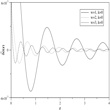
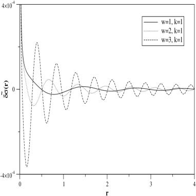
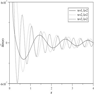
Figure 1: Profiles of the energy density perturbation amplitudes of the isotropic Schwarzschild thin disk with parameters (a=0.5,m=0.4). The first three different $w$ modes for the first three wave number $k$ are plotted, we see that increasing the $w$ mode the number of oscillations within the disk increases while increasing the wave number $k$ the amplitude decreases.

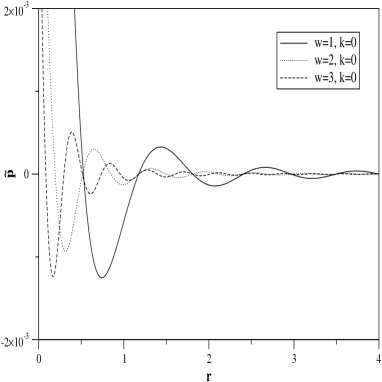
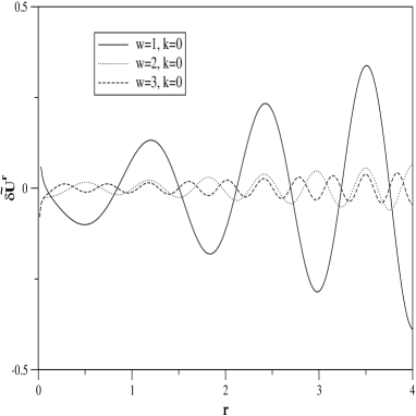
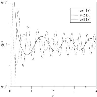
Figure 2: Profiles of the true pressure perturbation, physical radial velocity and physical azimuthal velocity amplitudes of the isotropic Schwarzschild thin disk with parameters (a=0.5,m=0.4). We see that the qualitative aspects of the pressure perturbation are the same of the energy density perturbation. The amplitude of the radial velocity increases when we get near the edge of the disk, in that circumstances we must compared these velocity values to the particle escape velocity to make the perturbation consistent with the model. The azimuthal velocity amplitude is almost constant far from the center of the disk.

III Thin disks with radial and azimuthal pressures

We start analyzing the isotropic Schwarzschild thin disk. This disk is found by setting the metric functions ($\Psi_{1},\Psi_{2},\Psi_{3}$) in (1) as

$$\Psi_{1}=\ln\left[\frac{2R-m}{2R+m}\right],$$

$$\Psi_{2}=\Psi_{3}=\ln\left[1+\frac{m}{2R}\right]^{2},$$ (25)

where $m$ is a positive constant and $R^{2}=r^{2}+(|z|+a)^{2}$, and applying the displace, cut and reflect method to the resulting isotropic Schwarzschild metric. With this operation, we find a thin disk with surface energy density and equal pressures given by vog:let ,

$$\sigma=\frac{16maR_{0}^{2}}{\pi(m+2R_{0})^{5}},$$ (26)

$$p=p_{r}=p_{\varphi}=-\frac{8m^{2}aR_{0}^{2}}{\pi(m+2R_{0})^{5}(m-2R_{0})},$$ (27)

where $R_{0}$ means to evaluate $R$ at $z=0$. Recall that we are not using the true fluid quantities, the quantities (26) and (27) are related to the ones cited in vog:let by Eqs. (16). From here and through the rest of the manuscript, all the calculations are made in the variables ($\sigma,p_{r},p_{\varphi}$) and the final results presented in the figures expressed in terms of the true physical variables.

We want our perturbations to be in accordance with the equation of state of the fluid, i.e. $p=p(r)$ and $\sigma=\sigma(r)$. Thus, $\delta p_{r}$ and $\delta\sigma$ satisfy

$$\delta p=\delta p_{r}=\delta p_{\varphi}=p_{,r}{\rm d}r,$$ (28)

$$\delta\sigma=\sigma_{,r}{\rm d}r,$$ (29)

from which we find the useful relation

$$\delta p=\left(\frac{p_{,r}}{\sigma_{,r}}\right)\delta\sigma.$$ (30)

Substituting $\delta U^{r}$ and $\delta U^{\varphi}$ in Eq. (22) from Eqs. (23) and (24), and using relation (30), we find a second order differential equation for the energy density perturbation $\delta\sigma$ of the form

$$A_{S}\delta\sigma_{,rr}+B_{S}\delta\sigma_{,r}+C_{S}\delta\sigma=0,$$ (31)

where ($A_{S},B_{S},C_{S}$) are functions of ($r,a,m,w,k_{\varphi}$), see Appendix A.

Note that the exact thin disk metrics we are considering are infinite in the radial direction. So, in order to study the stability of the disks we need a criterion to make a cut-off in the radial coordinate to create a finite disk. From vog:let we see that the energy density of the disks decreases rapidly enough in principle to define a cut-off radius. The cut-off radius $R_{cut}$ of the disk is set by the following criterion: the matter within the thin disk formed by the cut-off radius is more than 90% of the total energy density of the infinite disk. The other 10% of the energy density is distributed along the plane $z=0$ from outside the disk to infinity. This allow us, if necessary, to treat the outer 10% of the energy density disk as a perturbation in the outmost boundary condition. Moreover, the values of the parameters ($a,m$) of the finite disk we create must satisfy the dominant energy condition. For the infinite disk, this condition imposes that $\tilde{\sigma}+\tilde{p_{r}}+\tilde{p_{\varphi}}>0$ for all $r$. This inequality is valid in all the disk if $m<a$, the lower the value of $a$ for a given $m$ the faster the surface energy density decreases. Furthermore, this condition also implies that no tachyonic matter is present in the disk and that $p_{r}$ and $p_{\varphi}$ are in fact pressures and not tensions.

The second order equation (31) is solved with two boundary conditions, one in $r\approx 0$ and the other in the cut-off radius set by the criterion established above. At $r\approx 0$ we set the perturbation to be $\approx 10\%$ of the unperturbed energy density value and at the edge of the disk $\delta\sigma|_{r=R_{cut}}=0$. The last condition is imposed because we want the perturbation to vanish when $r$ tends to the outer radius.

Now, we consider the isotropic Schwarzschild thin disk with parameters ($a=0.5,m=0.4$). With these parameters, the outer radius of the disk is set to $r=4$ (approximately 90% of the energy density is inside the disk). In Fig. 1 we show the amplitude profiles of the true energy density perturbation $\tilde{\delta\sigma}$ for different modes of the perturbation (21). We see from Fig. 1 that the energy density perturbation profiles are stable and have an oscillatory character. When we increase the parameter $w$ the number of oscillations within the disk increases and when we increase the wave number $k$ the amplitude of the oscillations decreases. Note that the amplitudes of the modes decay quickly when we increase the value of the wave number. From Fig. 1 we see that there is a factor of approximately $10^{-3}$ between the modes $(w=1,k=0)$ and $(w=1,k=2)$.

In Fig. 2, we present the amplitude profiles of the true pressure perturbation and the physical radial velocity perturbation ($\tilde{\delta U^{r}}=\delta U^{r}\sqrt{g_{rr}}$) for the first three $w$ modes with $k=0$, and the amplitude profile of the physical azimuthal velocity perturbation ($\tilde{\delta U^{\varphi}}=\delta U^{\varphi}\sqrt{g_{\varphi\varphi}}$) for the first three $w$ modes with $k=1$. The modes of the azimuthal velocity perturbation with $k=0$ are equal to zero. We see from Fig. 2 that the pressure perturbation has the same qualitative aspects of the density perturbation. The azimuthal velocity perturbation amplitude shows an oscillatory behavior but the difference between it and the radial velocity perturbation is that after the first oscillations the maximum value of the amplitude remains almost constant for the rest of the disk. Note that the amplitude of the radial velocity perturbation increases with the radial coordinate. To discuss about this fact, we have to take into account that we are using in our numerical calculations a finite disk instead of the infinite disk exact solution. In the infinite disk there is no place for stars to escape from it but in the finite disk this could happen. For our disk to be consistent, the values of the radial velocity perturbation within the disk can not be greater than the particle escape velocity. In first approximation, the escape velocity of our disk is calculated using Newtonian mechanics. In the Newtonian limit of General Relativity, we have the well known relation $g_{00}=\eta_{00}+2\Phi$ and the particle escape velocity $V_{e}=\sqrt{2|\Phi|}$ can be written as

$$V_{e}=\left(1-\frac{(1-\frac{m}{2R})^{2}}{(1+\frac{m}{2R})^{2}}\right)^{1/2}.$$ (32)

For ($a=0.5,m=0.4,r=4$) the escape velocity is $\approx 0.42$ and we see from the radial velocity perturbation profile of Fig. 2 that the particles within the disk do not escape. In the case when the outer radius is equal to 5 (approximately 92% of the energy density) and the same parameters and perturbations are set, the escape velocity is $\approx 0.38$ and some modes of the radial velocity perturbation violates the consistency of the disk and can not exist. In other words, these modes describe a disk of a certain cut-off radius with no particles inside.

The case studied in this section corresponds to an extreme disk because the radial velocity of the particles at the cut-off radius are near the particle escape velocity. This example was chosen by didactic reasons to show the problems that may appear in finding a consistent finite disk model, but in most of the cases these problems do not appear. Recall that the perturbation made to the energy density was 10% of its unperturbed initial density. If we limited our perturbation to lower values, the radial velocity perturbation through the disk is below the escape velocity. Furthermore, we can define the cut-off radius of the disk when the energy density within the disk is lower than 90%. With lower values for the center perturbation and percentage of energy density within the disk, all modes tested were stable. The phenomenon of particles escaping from the disk is more suitable to occur in the mode with $(k=0,w=1)$. We see from Fig. 1 and Fig. 2 that increasing the number of the wave vector $k$ the amplitude of the variables considered decreases. All these considerations suggest that the isotropic Schwarzschild thin disk is stable under a general first order perturbation of the form (21) and favors the formation of rings.

When we performed the radial cut in the infinite disk in order to create the finite disk, we laid outside a fraction of the total energy density distributed up to infinity. We can model the presence of this exterior energy density, if necessary, by perturbing the outer boundary condition, i.e., setting in the outer radius the condition $\delta\sigma|_{r=R_{cut}}=\epsilon$ where $\epsilon\ll\delta\sigma|_{r=0}$. The numerical experiments realized show that this outer perturbation does not modify the qualitative aspects of our solutions. However, depending on the value of the perturbation, the quantitative aspects do change, but the disk remains stable.

IV Thin disks with only azimuthal pressure

IV.1 Chazy-Curzon thin disk

The Chazy-Curzon thin disk in Weyl coordinates bic:lyn has only azimuthal pressure, the absence of a radial pressure turns this solution rather unphysical. Even though, one can argue that the stability of the system can be achieved if we have two circular streams of particles moving in opposite directions, i.e. the counter-rotating hypothesis. Furthermore, the dragging of inertial frame of a rotating disk does not generate a Weyl type metric but the counter-rotating hypothesis solve this problem. Recently, evidence of disks made of streams of rotating and counter-rotating matter has been found ber . Also, a detailed study of the counter-rotating model for generic finite axially symmetric thin disk without radial pressure can be found in Ref. gon:esp .

The Chazy-Curzon metric is obtained from (1) with

$$\Phi=-\frac{m}{R},$$

$$\Lambda=-\frac{m^{2}r^{2}}{2R^{4}},$$ (33)

where $R^{2}=r^{2}+(|z|+a)^{2}$, and

$$\Psi_{1}=-\Psi_{2}=\Phi,$$

$$\Psi_{3}=\Lambda-\Phi.$$ (34)

The surface energy density and azimuthal pressure of the the Chazy-Curzon thin disk, after applying the image method to the metric (1) with the above definitions, are given by bic:lyn ,

$$\sigma=\frac{ma}{2\pi R_{0}^{3}}\left[1-\frac{m}{R_{0}}\left(1-\frac{a^{2}}{R_{0}^{2}}\right)\right]e^{2(\Phi_{0}-\Lambda_{0})},$$ (35)

$$p_{\varphi}=\frac{m^{2}a}{2\pi R_{0}^{4}}\left(1-\frac{a^{2}}{R_{0}^{2}}\right)e^{2(\Phi_{0}-\Lambda_{0})},$$ (36)

where $R_{0}$, $\Phi_{0}$ and $\Lambda_{0}$ are the respective functions evaluated at $z=0$. Since the Chazy-Curzon disk has no radial pressure, we have $p_{r}=\delta p_{r}=0$ in the perturbed equations. Substituting $\delta U^{r}$ and $\delta U^{\varphi}$ from Eqs. (23) and (24) into Eq. (22) and using a relation similar to (30) involving the fluid variables (35) and (36), we obtain a first order differential equation in $r$ for the perturbation $\delta\sigma$ of the form

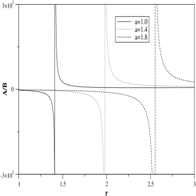
Figure 3: Profiles of the $A/B$ function present in the solution of the energy density perturbation for the thin Chazy-Curzon disk. The profiles show a singularity (instability) that depends on the cut parameter $a$. For $a=(1;\;1.4;\;1.8)$ and $m=1$, the singularities are approximately at $(1.414;\;1.980;\;2.546)$ respectively.

$$A\delta\sigma_{,r}+B\delta\sigma=0,$$ (37)

where ($A,B$) are functions of ($r,a,m,w,k_{\varphi}$), see Appendix B. The above equation has for solution

$$\delta\sigma=e^{\int(A/B){\rm d}r}.$$ (38)

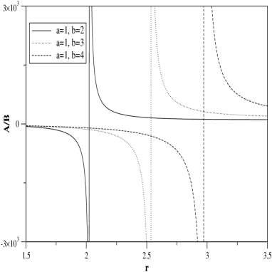
Figure 4: Profiles of the $A/B$ function present in the solution of the energy density perturbation for the thin Zipoy-Voorhees disk. As the Chazy-Curzon case, the profiles show a singularity (instability) that depends on the cut parameters $(a,b)$. For $b=(2;\;3;\;4)$, $a=1$ and $m=1$, the singularities are approximately at $(2.193;\;2.523;\;2.978)$ respectively.

In the integral argument, the values of ($a,m$) must satisfy the dominant energy condition $\tilde{\sigma}+\tilde{p_{\varphi}}>0$ for all $r$ if we want a fluid made of matter with the usual gravitational attractive property. This inequality is satisfied if $m/a\leq 3\sqrt{3}/4\approx 1.30$. In the case of the Chazy-Curzon disk, the dominant energy condition implies that the velocity of the counter-rotating streams does not exceed the velocity of light. We show in Fig. 3 the profile of the integral argument $A/B$ present in the solution (38) for different value of the parameter $a$. The singular points do not depend on the values of the parameters ($m,w,k_{\varphi}$) but on the value of the cut parameter $a$. The numerical experiments realized for the true surface energy density $\tilde{\delta\sigma}$ show instabilities at the same values of the singularities present in the function $A/B$. As far as we can test, the Chazy-Curzon disk does not allow any stable mode under perturbations of the form (21). Stability can be achieved if we let $p_{r}=0$ and $\delta p_{r}\neq 0$, but in this case is being changed the state equation of the fluid on the disk.

IV.2 Zipoy-Voorhees thin disk

In this section we study the stability of the Zipoy-Voorhees thin disks. These disks are obtained from the Zipoy-Voorhees metric, also known as the $\gamma$-metric. This metric represents, in Weyl coordinates, a uniform rod of length $b-a$ at a distance $a$ below the $z=0$ plane along the negative $z$ axis. The Zipoy-Voorhees metric is obtained from (1) with

$$\Phi=\frac{m}{b-a}\ln\left[\frac{R_{a}+|z|+a}{R_{b}+|z|+b}\right],$$

$$\Lambda=\frac{2m^{2}}{(b-a)^{2}}\ln\left[\frac{(R_{a}+R_{b})^{2}-(b-a)^{2}}{4R_{a}R_{b}}\right],$$ (39)

where $R_{a}^{2}=r^{2}+(|z|+a)^{2}$ and $R_{b}^{2}=r^{2}+(|z|+b)^{2}$, and

$$\Psi_{1}=-\Psi_{2}=\Phi,$$

$$\Psi_{3}=\Lambda-\Phi.$$ (40)

When $(b-a)=m$, the above solution leads to the Schwarzschild metric and when $(b-a)\rightarrow 0$, to the Chazy-Curzon solution. The thin disk formed by applying the displace, cut and reflect method has the surface energy density and the azimuthal pressure given by bic:lyn ,

$$\sigma=\frac{m}{2\pi(b-a)}\left(\frac{1}{R_{a0}}-\frac{1}{R_{b0}}\right)$$ (41)

$$\hskip 42.67912pt\left[1-\frac{m}{b-a}\left(\frac{b}{R_{b0}}-\frac{a}{R_{a0}}\right)\right]e^{2(\Phi_{0}-\Lambda_{0})},$$

$$p_{\varphi}=\frac{m^{2}}{2\pi(b-a)^{2}}\left(\frac{1}{R_{a0}}-\frac{1}{R_{b0}}\right)$$ (42)

$$\hskip 42.67912pt\left(\frac{b}{R_{b0}}-\frac{a}{R_{a0}}\right)e^{2(\Phi_{0}-\Lambda_{0})},$$

where $b\geq a$ and $R_{a0}$, $R_{b0}$, $\Phi_{0}$ and $\Lambda_{0}$ are the respective quantities evaluated at $z=0$. Like the Chazy-Curzon metric, these disks do not have radial pressure and, in order to generate a Weyl type metric, the counter-rotating hypothesis is applied.

Following the same steps as in the Chazy-Curzon metric, we arrive to a first order differential equation that yields a solution of the form (38). In this case, the values of the parameters ($a,b,m$) must satisfy the dominant energy condition $\tilde{\sigma}+\tilde{p_{\varphi}}>0$. To achieve this condition we must have bic:lyn ,

$$\frac{m}{b-a}\leq\frac{1}{2}\left(\frac{R_{b0}R_{a0}}{bR_{a0}-aR_{b0}}\right),$$ (43)

when

$$r^{2}=b^{2}\left(\frac{a}{b}\right)^{2/3}\left[1+\left(\frac{a}{b}\right)^{2/3}\right].$$ (44)

In Fig. 4 we plot the profiles of the integral argument $A/B$ for the Zipoy-Voorhees disk for different values of the parameter $b$. As the Chazy-Curzon disks, the singular points that appear in the profiles do not depend on the values of ($m,w,k_{\varphi}$) but on the value of the cut parameters $(a,b)$. Also, numerical experiments show that the true surface energy density is not stable at the same values of the singularities present in the function $A/B$. Moreover, under perturbation of the form (21), the Zipoy-Voorhees disk does not have any stable mode. A different treatment of the stability of the Chazy-Curzon and Zipoy-Voorhees thin disks bic:lyn , made by analyzing their velocity curves and specific angular momentum, shows that they are not stable for highly relativistic disks.

V Conclusions

We study the stability of several thin disk models in the context of General Relativity using a general first order perturbation. The stability analysis performed in this work is better than the stability analysis of particle motion along geodesics because we take into account the collective behavior of the particles. However, this analysis can be said to be incomplete because the energy momentum perturbation is treated like a test fluid and does not alter the background metric. The complete analysis of the thin disks stability needs to take into account the perturbation of the metric. This is a second degree of approximation to the stability problem in which the emission of gravitational radiation is considered.

We show that the Chazy-Curzon and Zipoy-Voorhees thin disks are not stable under perturbations of the form (21). This is due to the fact that there is no radial pressure to support the gravitational attraction of the disk. This appears to be in contradiction with the experimental evidence of stellar systems made of streams of rotating and counter-rotating matter ber , but the counter-rotating hypothesis assumes the existence of two pressureless streams of matter in circular opposite orbits which do not interact, see appendix of Ref. let2 , and this is not the case.

In the case of the isotropic Schwarzschild thin disk, where we have radial and azimuthal pressures, we formed a finite disk by making a cut-off radius and allowing a percentage of the unperturbed energy density within the disk. The finiteness of our new disk allows the particles to escape from it, so we have to compare the particles escape velocity with the velocity perturbation profiles if we want to have a self-consistent finite thin disk model or if we want to discard some perturbation modes. If we lower the value of the initial perturbation and/or the percentage of the total energy density inside the disk, all the modes are stable. The fluid variables, in the isotropic Schwarzschild thin disk, present an oscillatory character with the amplitudes vanishing when $r$ approaches the outmost radius. In the case of the azimuthal perturbation, the amplitude is almost constant within the disk. In general, when we increase the parameter $w$ the number of oscillations increases inside the disk and the amplitudes decrease. When we increase the wave number $k$ the values of the amplitudes decrease abruptly. We note that the perturbation (21) made in the isotropic Schwarzschild thin disk favors the formation of rings. As expected, the presence of a radial pressure is fundamental to the stability of thin disks.

APPENDIX A: COEFFICIENTS OF THE ISOTROPIC SCHWARZSCHILD THIN DISK SECOND ORDER PERTURBATION EQUATION

The general form of the functions $(A_{S},B_{S},C_{S})$ appearing in the second order equation (31) are given by

$$A_{S}=A_{1}\alpha_{1},$$

$$B_{S}=A_{1}(\alpha_{1,r}+\alpha_{2})+A_{2}\alpha_{1},$$

$$C_{S}=A_{1}\alpha_{2,r}+A_{2}\alpha_{2}+A_{3}\alpha_{3}+A_{4},$$ (45)

where $\alpha_{1}$, $\alpha_{2}$ and $\alpha_{3}$ are

$$\alpha_{1}=-\frac{f_{,r}B_{1}+f(B_{4}+B_{5})+B_{3}}{B_{2}},$$

$$\alpha_{2}=-\frac{fB_{1}}{B_{2}},$$

$$\alpha_{3}=-\frac{fC_{2}}{C_{1}},$$ (46)

and $f=(p_{,r}/\sigma_{,r})$. In Eqs. (45) and (46), we denote the coefficients of Eq. (22) by $A_{i}$, the coefficients of Eq. (23) by $B_{i}$ and the coefficients of Eq. (24) by $C_{i}$, e.g., the first term in (22) has the coefficient $A_{1}$ multiplied by the factor $\delta U^{r}_{,r}$, the second term has the coefficient $A_{2}$ multiplied by the factor $\delta U^{r}$, etc.

The explicit form of the above equations are obtained substituting the fluid variables ($p,\sigma$) of the isotropic Schwarzschild thin disk.

APPENDIX B: ARGUMENT $(A/B)$ OF THE INTEGRAL (38)

The general form of the argument $(A/B)$ of the integral Eq. (38) are given by

$$A=\sigma U^{t}\alpha_{1,r}+{\rm F}(t,r,\sigma U^{t})\alpha_{1}$$

$$\hskip 22.76228pt-k_{\varphi}(\sigma U^{t}+\xi_{2}p_{\varphi}Y^{\varphi})\alpha_{2}+wU^{t}U^{t},$$

$$B=\sigma U^{t}\alpha_{1},$$ (47)

where the functions $\alpha_{1}$ and $\alpha_{2}$ are

$$\alpha_{1}=\frac{U^{t}U^{t}\Gamma^{r}_{tt}+Y^{\varphi}Y^{\varphi}\Gamma^{r}_{\varphi\varphi}(p_{\varphi,r}/\sigma_{,r})}{w\sigma U^{t}}$$ (48)

$$\alpha_{2}=\frac{k_{\varphi}Y^{\varphi}Y^{\varphi}}{w(\sigma U^{t}+\xi_{2}p_{\varphi}Y^{\varphi})}.$$ (49)

The explicit form of the above equations are obtained substituting the particular fluid variables ($p_{\varphi},\sigma$) of the Chazy-Curzon or Zipoy-Voorhees thin disks.

References

- (1) W.A. Bonnor and A. Sackfield, Commun. Math. Phys. 8, 338 (1968).
- (2) T. Morgan and L. Morgan, Phys. Rev. 183, 1097 (1969).
- (3) L. Morgan and T. Morgan, Phys Rev. D 2, 2756 (1970).
- (4) G. González and P.S. Letelier, Class. Quantum Grav. 16, 479 (1999).
- (5) T. Ledvinka, M. Zofka, and J. Bičák, in Proceedings of the 8th Marcel Grossman Meeting in General Relativity, edited by T. Piran (World Scientific, Singapore, 1999), pp. 339-341.
- (6) P.S. Letelier, Phys. Rev. D 60, 104042 (1999).
- (7) J. Katz, J. Bičák and D. Lynden-Bell, Class. Quantum Grav. 16, 4023 (1999).
- (8) D. Lynden-Bell and S. Pineault, Mon. Not. R. Astron. Soc. 185, 679 (1978).
- (9) J.P.S. Lemos, Class. Quantum Grav. 6, 1219 (1989).
- (10) J.P.S. Lemos and P.S. Letelier, Class. Quantum Grav. 10, L75 (1993).
- (11) J.P.S. Lemos and P.S. Letelier, Phys. Rev. D 49, 5135 (1994).
- (12) J.P.S. Lemos and P.S. Letelier, Int. J. Mod. Phys. D 5, 53 (1996).
- (13) C. Klein, Class. Quantum Grav. 14, 2267 (1997).
- (14) J. Bičák and T. Ledvinka, Phys. Rev. Lett. 71, 1669 (1993).
- (15) J. Bičák, D. Lynden-Bell and J. Katz, Phys. Rev. D 47, 4334 (1993).
- (16) M. Chazy, Bull. Soc. Math. France 52, 17 (1924).
- (17) H. Curzon, Proc. London Math. Soc. 23, 477 (1924).
- (18) D.M. Zipoy, J. Math. Phys. 7, 1137 (1966).
- (19) B.H. Voorhees, Phys. Rev. D 2, 2119 (1970).
- (20) J. Bičák, D. Lynden-Bell and C. Pichon, Mon. Not. R. Astron. Soc. 265, 126 (1993).
- (21) D. Vogt and P.S. Letelier, Phys. Rev. D 68, 084010 (2003).
- (22) D. Vogt and P.S. Letelier, Class. Quantum Grav. 21, 3369 (2004)
- (23) D. Vogt and P.S. Letelier, Exact Relativistic Static Charged Perfect Fluid Disks, Phys. Rev. D (in press).
- (24) G.A. González and P.S. Letelier, Phys. Rev. D 69, 044013 (2004).
- (25) O. Semerák, in Gravitation: Following the Prague Inspiration, to Celebrate the 60th Birthday of Jiri Bičák, edited by O. Semerák, J. Podolsky, and M. Zofka (World Scientific, Singapure, 2002), p. 111, available at http://xxx.lanl.gov/abs/gr-qc/0204025.
- (26) J. Binney and S. Tremaine, Galactic Dynamics, (Princeton University Press, New Jersey, 1987).
- (27) A.M. Fridman and V.L. Polyachenko, Physics of Gravitating Systems I : Equilibrium and Stability, (Springer-Verlag, New York, 1984).
- (28) Lord Rayleigh, Proc. R. Soc. London A93, 148 (1916).
- (29) L.D. Landau and E.M. Lifshitz, Fluid Mechanics, 2nd ed. (Pergamon Press, Oxford, 1987), Sec. 27.
- (30) P.S. Letelier, Phys. Rev. D 68, 104002 (2003).
- (31) H.A. Buchdahl, Astrophys. J. 140, 1512 (1964).
- (32) V.V. Narlikar, G.K. Patwardhan and P.C. Vaidya, Proc. Natl. Inst. Sci. India 9, 229 (1943).
- (33) J.M. Bardeen, Astrophys. J. 161, 103 (1970).
- (34) M.A. Abramowicz and A.R. Prasanna, Mon. Not. R. Astron. Soc. 245, 720 (1990).
- (35) O. Semerák and M. Žáček, Publ. Astron. Soc. Japan 52, 1067 (2000).
- (36) O. Semerák and M. Žáček, Class. Quantum Grav. 17, 1613 (2000).
- (37) O. Semerák, Class. Quantum Grav. 20, 1613 (2003).
- (38) F.H. Seguin, Astrophys. J. 197, 745 (1975).
- (39) F. Bertotal et al., Astrophys. J. Lett. 458, L67 (1996).
- (40) G.A. González and O.A. Espitia, Phys. Rev. D 68, 104028 (2003).