Exact Relativistic Static Charged Perfect Fluid Disks

Abstract

Using the well-known “displace, cut and reflect” method used to generate disks from given solutions of Einstein field equations, we construct static charged disks made of perfect fluid based on the Reissner-Nordström solution in isotropic coordinates. We also derive a simple stability condition for charged and non charged perfect fluid disks. As expected, we find that the presence of charge increases the regions of instability of the disks.

I Introduction

Axisymmetric solutions of Einstein field equations corresponding to disklike configurations of matter have been extensively studied. These solutions can be static or stationary and with or without radial pressure. Solutions for static thin disks without radial pressure were first studied by Bonnor and Sackfield Bonnor1 , and Morgan and Morgan Morgan1 , and with radial pressure by Morgan and Morgan Morgan2 . Other classes of static thin disk solutions have been obtained Lynden1 –Bicak2 , while stationary thin disks were studied in Bicak3 –Gonzalez1 . Also thin disks with radial tension Gonzalez2 , magnetic fields Letelier1 and both electric and magnetic fields Katz1 have been studied. An exact solution to the problem of a rigidly rotating disk of dust in terms of ultraelliptic functions was reported in Neugebauer , while models of static relativistic counterrotating dust disks were recently presented in Gonzalez3 . Structures of nonaxisymmetric matter distributions of static charged dust were also recently studied Vogt2 . The non-linear superposition of a disk and a black hole was first considered by Lemos and Letelier Lemos2 . Models of thin disks and thin disks with halos made of perfect fluids were considered in Vogt . The generalization of the “displace, cut and reflect” method (Sec. II) to construct thick static disks was considered by González and Letelier Gonzalez4 . For a recent review on relativistic accretion disks see Karas .

Gravitationally bound stellar objects are likely to be positively charged due to the fact that the electrons are lighter than the protons so the formers can more easily scape from the stellar object. One should expect to have an equilibrium situation when the electrostatic energy of the electron ($eV$) is of the order of its thermal energy ($kT$) Bally , then the scape would stop. Similar considerations can be found in Ref. Shvartsman .

The aim of this paper is to present a charged version of perfect fluid disks that were studied in Vogt . They are constructed with the well known “displace, cut and reflect” method applied to the Reissner-Nordström metric in isotropic coordinates. The stability of these new model of charged disks will also be considered. We present and extension of the Rayleigh criteria of stability Rayleigh for the case of relativistic disks made of a charged perfect fluid. We find a simple condition to have gravitationally bounded disks.

The paper is divided as follows. Sec. II discusses the formalism which can be used to construct disks given a solution of Einstein-Maxwell equations, and the main physical variables of the disk. In Sec. III Rayleigh inspired criteria of stability criteria for the stability of charged and noncharged perfect fluid disks is established. The properties and stability of the charged disks are discussed in Sec. IV. Finally, in Sec. V, we discuss our results and make some considerations about the construction of charged perfect fluid disks with halos. The “displace, cut and reflect” method is reviewed in an Appendix.

II Einstein-Maxwell Equations and Disks

The isotropic metric representing a static spherically symmetric space-time can be expressed as

$$\mathrm{d}s^{2}=e^{\nu(r)}\mathrm{d}t^{2}-e^{\lambda(r)}(\mathrm{d}r^{2}+r^{2}d\Omega^{2}),$$ (1)

where $d\Omega^{2}=\mathrm{d}\theta^{2}+\sin^{2}\theta\mathrm{d}\varphi^{2}$. The same metric in cylindrical coordinates $(t,R,z,\varphi)$ reads:

$$\mathrm{d}s^{2}=e^{\nu(R,z)}\mathrm{d}t^{2}-e^{\lambda(R,z)}\left(\mathrm{d}R^{2}+\mathrm{d}z^{2}+R^{2}\mathrm{d}\varphi^{2}\right)\mbox{.}$$ (2)

The Einstein-Maxwell system of equations is given by

$$G_{\mu\nu} =8\pi T_{\mu\nu}\mbox{,}$$ (3)

$$T_{\mu\nu} =\frac{1}{4\pi}\left(F_{\mu}{}^{\sigma}F_{\nu\sigma}+\frac{1}{4}g_{\mu\nu}F_{\rho\sigma}F^{\rho\sigma}\right)\mbox{,}$$ (4)

$$F^{\mu\nu}{}_{;\mu} =0\mbox{,}$$ (5)

$$F_{\mu\nu} =A_{\nu,\mu}-A_{\mu,\nu}\mbox{,}$$ (6)

where all symbols have their usual meaning. We use geometric units with $G=c=1$.

The method used to generate the metric of the disk and its material content is the well known “displace, cut and reflect” method (see the Appendix) that was first used by Kuzmin Kuzmin and Toomre Toomre to construct Newtonian models of disks, and later extended to general relativity (see, for example Bicak1 ; Gonzalez1 ). Given a solution of the Einstein-Maxwell equation, this procedure is mathematically equivalent to apply the transformation $z\rightarrow|z|+a$, with $a$ constant, on that solution. In the Einstein tensor we have first and second derivatives of $z$. Remembering that $\partial_{z}|z|=2\vartheta(z)-1$ and $\partial_{zz}|z|=2\delta(z)$, where $\vartheta(z)$ and $\delta(z)$ are, respectively, the Heaviside function and the Dirac distribution, Einstein-Maxwell equations give us

$$G_{\mu\nu} =8\pi(T_{\mu\nu}^{\mathrm{elm.}}+Q_{\mu\nu}\delta(z))\mbox{,}$$ (7)

$$F^{\mu\nu}{}_{;\mu} =4\pi J^{\nu}\delta(z)\mbox{,}$$ (8)

where $T_{\mu\nu}^{\mathrm{elm.}}$ is the electromagnetic tensor Eq. (4), $Q_{\mu\nu}$ is the energy-momentum tensor on the plane $z=0$ and $J^{\nu}$ is the current density on the plane $z=0$. For the metric (2), the non-zero components of $Q_{\mu\nu}$ are

$$Q^{t}_{t} =\frac{1}{16\pi}\left[-b^{zz}+g^{zz}(b^{R}_{R}+b^{z}_{z}+b^{\varphi}_{\varphi})\right]\mbox{,}$$ (9)

$$Q^{R}_{R} =Q^{\varphi}_{\varphi}=\frac{1}{16\pi}\left[-b^{zz}+g^{zz}(b^{t}_{t}+b^{R}_{R}+b^{z}_{z})\right]\mbox{,}$$ (10)

where $b_{\mu\nu}$ denote the jump of the first derivatives of the metric tensor on the plane $z=0$,

$$b_{\mu\nu}=g_{\mu\nu,z}|_{z=0^{+}}-g_{\mu\nu,z}|_{z=0^{-}}\mbox{,}$$ (11)

and the other quantities are evaluated at $z=0^{+}$. The electromagnetic potential for an electric field is

$$A_{\mu}=(\phi,0,0,0)\mbox{.}$$ (12)

Using Eq. (12) and Eq. (8), the only non-zero component of the current density on the plane $z=0$ is

$$J^{t}=\frac{1}{4\pi}g^{zz}g^{tt}a_{t}\mbox{,}$$ (13)

where $a_{\mu}$ denote the jump of the first derivatives of the electromagnetic potential on the plane $z=0$,

$$a_{\mu}=A_{\mu,z}|_{z=0^{+}}-A_{\mu,z}|_{z=0^{-}}\mbox{,}$$ (14)

and the other quantities are evaluated at $z=0^{+}$. The “physical measure” of length in the direction $\partial_{z}$ for metric (2) is $\sqrt{-g_{zz}}$, then the invariant distribution is $\delta(z)/\sqrt{-g_{zz}}$. Thus the “true” surface energy density $\sigma$ and the azimuthal and radial pressures or tensions $(P)$ are:

$$\sigma=\sqrt{-g_{zz}}Q^{t}_{t}\text{,}\quad P=-\sqrt{-g_{zz}}Q^{R}_{R}=-\sqrt{-g_{zz}}Q^{\varphi}_{\varphi}\mbox{.}$$ (15)

Since $J^{\mu}=\rho U^{\mu}$, where $U^{\mu}=\delta^{\mu}_{t}/\sqrt{g_{tt}}$, the “true” surface charge density $\rho$ is

$$\rho=\sqrt{-g_{zz}g_{tt}}J^{t}\mbox{.}$$ (16)

III Stability Conditions for Perfect Fluid Disks

One way to explain stability of static disks without radial pressure is to assume that the particles on the disk plane move under the action of their own gravitational field in such a way that as many particles move clockwise as counterclockwise (counterrotating model). With this assumption, stability of the matter on the disk can be associated with stability of circular orbits along geodesics (see Letelier2 for a detailed explanation). The usual stability criteria for circular orbits is adapted from the Rayleigh criteria of stability for a rotating fluid Rayleigh . One finds that stability against small radial perturbations is achieved when

$$h\frac{dh}{dr}>0\mbox{,}$$ (17)

where $h$ is the specific angular momentum of the circular orbit.

In the case of perfect fluid disks the situation is somewhat different, since radial pressure can equilibrate the inward gravitational force and no counterrotating hypothesis is needed. Using $T^{\mu\nu}{}_{;\nu}=0$ where $T^{\mu\nu}$ is the sum of the energy-momentum tensor for a perfect fluid and Eq. (4), the equilibrium condition in the radial direction on the plane $z=0$ is given by

$$\frac{1}{2}(P+\sigma)(e^{\nu})_{,R}=-\rho e^{\nu/2}\phi_{,R}-e^{\nu}P_{,R}\mbox{.}$$ (18)

The left side of Eq. (18) can be interpreted as the gravitational force which equilibrates the pressure and electric forces that appear on the right side. Now suppose an element of fluid at radius $R$ is displaced to $R+\Delta R$ keeeping $P$, $\sigma$ and $\rho$ constant. The right side of Eq. (18) becomes

$$-e^{\nu(R+\Delta R)/2}\phi_{,R}(R+\Delta R)\rho(R)-e^{\nu(R+\Delta R)}P_{,R}(R)\mbox{.}$$ (19)

These “forces” should be compared with the right side of Eq. (18) at radius $R+\Delta R$:

$$-e^{\nu(R+\Delta R)/2}\phi_{,R}(R+\Delta R)\rho(R+\Delta R)$$

$$-e^{\nu(R+\Delta R)}P_{,R}(R+\Delta R)\mbox{.}$$ (20)

To have stability expression (19) must be less then expression (III). Expanding $\rho(R+\Delta R)$ and $P_{,R}(R+\Delta R)$ around $R$, we get

$$e^{\nu/2}\phi_{,R}\rho_{,R}+e^{\nu}P_{,RR}<0\mbox{.}$$ (21)

For an uncharged fluid, condition (21) reduces to $P_{,RR}<0$.

Note that this criterium of stability refers only to radial perturbations of the pressure and charge. It really gives us a condition to have gravitationally bounded systems. In other words the disks do not explode, but they can collapse. In the general case, the study stability of gravitating systems reduces to the much harder problem of the study of the eigenvalue problem for a nontrivial elliptic operator Friedman .

IV Charged Perfect Fluid Disks

We apply now the results of the previous sections to construct charged disks.The Reissner-Nordström solution in Schwarzschild coordinates is given by

$$\mathrm{d}s^{2}=\left(1-\frac{2m}{r}+\frac{Q^{2}}{r^{2}}\right)\mathrm{d}t^{2}-\frac{\mathrm{d}r^{2}}{\left(1-\frac{2m}{r}+\frac{Q^{2}}{r^{2}}\right)}-r^{2}d\Omega^{2}\mbox{,}$$ (22)

where $m$ and $Q$ are, respectively, the mass and charge of the black hole, and $m>Q$. The electromagnetic potential associated to solution (22) is

$$A_{\mu}=\left(\frac{Q}{r},0,0,0\right)\mbox{.}$$ (23)

With the radial coordinate transformation

$$r=r^{\prime}\left(1+\frac{m+Q}{2r^{\prime}}\right)\left(1+\frac{m-Q}{2r^{\prime}}\right)\mbox{,}$$ (24)

metric (22) and Eq. (23) can be expressed in isotropic coordinates $(t,r^{\prime},\theta,\varphi)$ as

$$\mathrm{d}s^{2}=\frac{\left[1-\frac{(m^{2}-Q^{2})}{4r^{\prime 2}}\right]^{2}}{\left[1+\frac{(m+Q)}{2r^{\prime}}\right]^{2}\left[1+\frac{(m-Q)}{2r^{\prime}}\right]^{2}}\mathrm{d}t^{2}-\left[1+\frac{(m+Q)}{2r^{\prime}}\right]^{2}\left[1+\frac{(m-Q)}{2r^{\prime}}\right]^{2}(\mathrm{d}r^{\prime 2}+r^{\prime 2}\mathrm{d}\theta^{2}+r^{\prime 2}\sin^{2}\theta\mathrm{d}\varphi^{2})\mbox{,}$$ (25)

$$A_{\mu}=\left(\frac{Q}{r^{\prime}\left(1+\frac{m+Q}{2r^{\prime}}\right)\left(1+\frac{m-Q}{2r^{\prime}}\right)},0,0,0\right)\mbox{.}$$ (26)

Transforming Eq. (25)-(26) to cylindrical coordinates, and using Eq. (15) and (16), we obtain a disk with surface energy density $\sigma=\bar{\sigma}/m$, equal radial and azimuthal pressures (or tensions) $P=\bar{P}/m$ and surface charge density $\rho=\bar{\rho}/m$ where

$$\bar{\sigma} =\frac{4\tilde{a}}{\pi}\frac{2\sqrt{\tilde{R}^{2}+\tilde{a}^{2}}+1-\tilde{Q}^{2}}{[(1+2\sqrt{\tilde{R}^{2}+\tilde{a}^{2}})^{2}-\tilde{Q}^{2}]^{2}}\mbox{,}$$ (27)

$$\bar{P} =-\frac{2\tilde{a}}{\pi}\frac{1-\tilde{Q}^{2}}{[(1+2\sqrt{\tilde{R}^{2}+\tilde{a}^{2}})^{2}-\tilde{Q}^{2}][1-\tilde{Q}^{2}-4(\tilde{R}^{2}+\tilde{a}^{2})]}\mbox{,}$$ (28)

$$\bar{\rho} =\frac{8\tilde{Q}\tilde{a}\sqrt{\tilde{R}^{2}+\tilde{a}^{2}}}{\pi\left[4\sqrt{\tilde{R}^{2}+\tilde{a}^{2}}(1+\sqrt{\tilde{R}^{2}+\tilde{a}^{2}})+1-\tilde{Q}^{2}\right]^{2}}\mbox{,}$$ (29)

with $\tilde{R}=R/m$, $\tilde{a}=a/m$ and $\tilde{Q}=Q/m$.

Eq. (27) shows that the disk’s surface density is always positive (weak energy condition) for $\tilde{Q}<1$. Positive values (pression) for the stresses in azimuthal and radial directions are obtained if $\tilde{a}>\sqrt{1-\tilde{Q}^{2}}/2$. The velocity of sound propagation $V$, defined as $V^{2}=\frac{dP}{d\sigma}$, is calculated using Eq. (27) and Eq. (28):

$$V^{2}=\frac{(1-\tilde{Q}^{2})[(1+2\sqrt{\tilde{R}^{2}+\tilde{a}^{2}})^{2}-\tilde{Q}^{2}][(1+2\sqrt{\tilde{R}^{2}+\tilde{a}^{2}})^{2}(1-4\sqrt{\tilde{R}^{2}+\tilde{a}^{2}})-\tilde{Q}^{2}]}{[1-\tilde{Q}^{2}-4(\tilde{R}^{2}+\tilde{a}^{2})]^{2}[-3(1+2\sqrt{\tilde{R}^{2}+\tilde{a}^{2}})^{2}+\tilde{Q}^{2}(3+8\sqrt{\tilde{R}^{2}+\tilde{a}^{2}})]}\mbox{.}$$ (30)

Fig. 1 shows the curves of $V^{2}=1$ (solid curve) and of $\tilde{a}=\sqrt{1-\tilde{Q}^{2}}/2$ (dotted curve) where $\bar{P}$ changes sign as functions of the parameters $\tilde{a}=a/m$ and $\tilde{Q}=Q/m$. Above the dotted curve, stresses are positive (pressure) for all $\tilde{R}$ and above the solid curve, condition $V^{2}<1$ is also satisfied for all $\tilde{R}$. Thus, choosing values for $\tilde{a}$ and $\tilde{Q}$ that lie above the solid curve ensures that the entire disk will have pressures and sublumial sound velocities. We also note that with increasing charge the range of the cut parameter $a$ that generates disks for which the conditions stated above are satisfied is enlarged.

Figure 1: Curve $V^{2}=1$ (solid curve) as a function of the parameters $\tilde{a}=a/m$ and $\tilde{Q}=Q/m$ for the charged disk of perfect fluid. Also $\tilde{a}=\sqrt{1-\tilde{Q}^{2}}/2$ (dotted curve).

Fig. 2 (a)–(d) shows, respectively, the surface energy density $\bar{\sigma}$, pressures $\bar{P}$, sound velocity $V$ and charge density $\bar{\rho}$ with $\tilde{a}=1$, $\tilde{Q}=0$, $0.3$, $0.6$ and $0.9$ as functions of $\tilde{R}$. As charge increases, the disks become less relativistic for the same cut parameter; energy density and pressures are lowered and charge density becomes more concentrated near the disk center.

Figure 2: (a) The surface energy density $\bar{\sigma}$, Eq. (27), (b) the pressure $\bar{P}$, Eq. (28), (c) the sound velocity $V$ Eq. (30) and (d) the charge density $\bar{\rho}$, Eq. (29) for the disk with $\tilde{a}=1$, $\tilde{Q}=0$, $0.3$, $0.6$ and $0.9$ as functions of $\tilde{R}$.

Fig. 3(a) is a graph of curves where Eq. 21 changes sign. The curves have been plotted only for ranges of parameter $\tilde{a}$ where $V^{2}<1$ (Fig. 1). At the left of each curve, stability condition (21) is satisfied. Thus the disks are stable only in a small region near their centers. We also note that the charge decreases the radii of stability. The left side of Eq. 21 is plotted in Fig. 3(b) for the same parameters as in Fig. 2.

Figure 3: (a) Curves where Eq. (21) defining stability changes sign as functions of radius $\tilde{R}$, cut parameter $\tilde{a}$ and charge $\tilde{Q}$. Disks are stable at the left of each curve. (b) Curves of the left side of Eq. (21) for the same parameters as in Fig. 2.

V Discussion

We applied the “displace, cut and reflect” method on the Reissner-Nordström solution in isotropic coordinates and generated static charged disks made of perfect fluid. We also derived a simple criteria for the stability for charged and uncharged perfect fluid disks that is an extension of the Rayleigh criteria of stability for rotating fluids. The addition of charge decreases the energy density and pressures near the disk’s centers, while charge density in enhanced there. Furthermore, presence of charge decreases the stable regions of the disks, that are reduced to small regions near the center even in the absence of charge. This is a rather different result from that of our previous stability analysis of the uncharged perfect fluid disk Vogt based on the stability study of circular orbits of test particles, where we found that the disks were completely stable for $\tilde{a}\gtrapprox 1.016$. It is worthwhile to note that the criteria used to study stability of disks made of counterrotating matter is based on a particle consideration, whereas the stability criteria derived for perfect fluid disks is based on collective phenomena. Therefore, the stability criteria derived in this paper seems to us to be more appropriate for the study of perfect fluid disks.

In principle it is possible to add charged halos to the disks presented in this work by applying the “displace, cut and reflect” method to a static charged sphere of perfect fluid in isotropic coordinates (see the Appendix). The halos could have charge of the same sign or opposite sign of the disk’s charge such that the entire object could be neutral or have an arbitrary charge. Although there exist many exact solutions for charged fluid spheres in Schwarzschild coordinates (see, for example, Ivanov ), we have not found in the literature similar solutions in isotropic coordinates. This may be due to the fact that in these coordinates the Einstein-Maxwell equations for a charged perfect fluid are reduced to a system of highly nonlinear coupled second order differential equations for both metric functions $\nu(r)$ and $\lambda(r)$ and for the electrostatic potential $\phi(r)$, so the task of finding exact solutions is more involved than in canonical spherical coordinates. We believe that this search for exact solutions in isotropic coordinates is worthwile.

*

Appendix A

In this appendix we give an overview of the “displace, cut and reflect” method used to generate the metric and its material and electric content from a known solution of the Einstein-Maxwell field equations. The method can be divided in the following steps that are illustrated in Fig. 4: First, in a space wherein we have a compact source of gravitational field, we choose a surface (in our case, the plane $z=0$) that divides the space in two pieces: one with no singularities or sources and the other with the sources. Then we disregard the part of the space with singularities and use the surface to make an inversion of the nonsingular part of the space. This results in a space with a singularity that is a delta function with support on $z=0$.

Figure 4: An illustration of the “displace, cut and reflect” method for the generation of disks. In A the spacetime with a singularity is displaced and cut by a plane (dotted line), in B the part with singularities is disregarded and the upper part is reflected on the plane.

The same procedure can be used with a static sphere of charged perfect fluid to generate charged disks with halos, as depicted in Fig. 5: the sphere is displaced and cut by a distance $a$ less then its radius. The part of the space that contains the center of the sphere is disregarded. After the inversion of the remaining space, one ends up with a charged disk surrounded by a cap of charged perfect fluid.

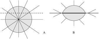
Figure 5: An illustration of the “displace, cut and reflect” method for the generation of charged disks with halos. In A the sphere of perfect fluid is displaced and cut by a plane (dotted line), in B the part that contains the center of the sphere is disregarded and the upper part is reflected on the plane.

If the internal fluid solution is matched to the Reissner-Nordström metric Eq. (25), the outer part of the disk will have the physical properties deduced in Sec. IV, while the properties of the inner part will depend on the particular fluid solution.

References

- (1) W. A. Bonnor and A. Sackfield, Commun. Math. Phys. 8, 338 (1968).
- (2) T. Morgan and L. Morgan, Phys. Rev. 183, 1097 (1969).
- (3) L. Morgan and T. Morgan, Phys. Rev. D 2, 2756 (1970).
- (4) D. Lynden-Bell and S. Pineault, Mon. Not. R. Astron. Soc. 185, 679 (1978).
- (5) J. P. S. Lemos, Class. Quantum Grav. 6, 1219 (1989).
- (6) J. Bičák, D. Lynden-Bell and J. Katz, Phys. Rev. D 47, 4334 (1993).
- (7) J. Bičák, D. Lynden-Bell and C. Pichon, Mon. Not. R. Astron. Soc. 265, 126 (1993).
- (8) J. Bičák and T. Ledvinka, Phys. Rev. Lett. 71, 1669 (1993).
- (9) T. Ledvinka, M. Zofka and J. Bičák, in Proceedings of the 8th Marcel Grossman Meeting in General Relativity, edited by T. Piran (World Scientific, Singapore, 1999), p. 339-341.
- (10) G. González and P. S. Letelier, Phys. Rev. D 62, 064025 (2000).
- (11) G. González and P. S. Letelier, Class. Quantum Grav. 16, 479 (1999).
- (12) P. S. Letelier, Phys. Rev. D 60, 104042 (1999).
- (13) J. Katz, J. Bičák and D. Lynden-Bell, Class. Quantum Grav. 16, 4023 (1999).
- (14) G. Neugebauer and R. Meinel, Phys. Rev. Lett. 75, 3046 (1995).
- (15) G. García R. and G. González, Phys. Rev. D 69, 124002 (2004).
- (16) D. Vogt and P. S. Letelier, Class. Quantum Grav. (in press).
- (17) J. P. S. Lemos and P. S. Letelier, Class. Quantum Grav. 10, L75 (1993).
- (18) D. Vogt and P. S. Letelier, Phys. Rev. D 68, 084010 (2003).
- (19) G. González and P. S. Letelier, Phys. Rev. D 69, 044013 (2004).
- (20) V. Karas, J.-M. Huré and O. Semerák, Class. Quantum Grav. 21, R1 (2004).
- (21) J. Bally and E.R. Harrison, Ap. J.220, 743 (1978).
- (22) V.F. Shvartsman,Soviet Physics, JETP 33, 475 (1971) [ Zh. Eksp. Teor. Fiz 60, 881 (1971)].
- (23) Lord Rayleigh, Proc. R. Soc. London A93, 148 (1917); see also L. D. Landau and E. M. Lifshitz, Fluid Mechanics, 2nd Ed. (Pergamon Press, Oxford, 1987), §27.
- (24) G. G. Kuzmin, Astron. Zh. 33, 27 (1956).
- (25) A. Toomre, Ap. J. 138, 385 (1962).
- (26) P. S. Letelier, Phys. Rev. D 68, 104002 (2003).
- (27) See for instance, A.N. Friedman and V.LK. Polyachenko, Physics of Gravitating Systems, (Springer-Verlag, New York, 1983).
- (28) B. V. Ivanov, Phys. Rev. D 65, 104001 (2002).