Bianchi type I universe with viscous fluid

Abstract

We study the evolution of a homogeneous, anisotropic Universe given by a Bianchi type-I cosmological model filled with viscous fluid, in the presence of a cosmological constant $\Lambda$. The role of viscous fluid and $\Lambda$ term in the evolution the BI space-time is studied. Though the viscosity cannot remove the cosmological singularity, it plays a crucial part in the formation of a qualitatively new behavior of the solutions near singularity. It is shown that the introduction of the $\Lambda$ term can be handy in the elimination of the cosmological singularity. In particular, in case of a bulk viscosity, it provides an everlasting process of evolution ($\Lambda<0$), whereas, for some positive values of $\Lambda$ and the bulk viscosity being inverse proportional to the expansion, the BI Universe admits a singularity-free oscillatory mode of expansion. In case of a constant bulk viscosity and share viscosity being proportional to expansion, the model allows oscillatory mode accompanied by an exponential growth even with a negative $\Lambda$. Space-time singularity in this case occurs at $t\to-\infty$.

I Introduction

The investigation of relativistic cosmological models usually has the energy momentum tensor of matter generated by a perfect fluid. To consider more realistic models one must take into account the viscosity mechanisms, which have already attracted the attention of many researchers. Misner mis1 ; mis2 suggested that strong dissipative due to the neutrino viscosity may considerably reduce the anisotropy of the blackbody radiation. Viscosity mechanism in cosmology can explain the anomalously high entropy per baryon in the present universe wein ; weinb . Bulk viscosity associated with the grand-unified-theory phase transition lang may lead to an inflationary scenario waga ; pacher ; guth .

A uniform cosmological model filled with fluid which possesses pressure and second (bulk) viscosity was developed by Murphy murphy . The solutions that he found exhibit an interesting feature that the big bang type singularity appears in the infinite past. Exact solutions of the isotropic homogeneous cosmology for open, closed and flat universe have been found by Santos et al santos , with the bulk viscosity being a power function of energy density.

The nature of cosmological solutions for homogeneous Bianchi type I (BI) model was investigated by Belinsky and Khalatnikov belin by taking into account dissipative process due to viscosity. They showed that viscosity cannot remove the cosmological singularity but results in a qualitatively new behavior of the solutions near singularity. They found the remarkable property that during the time of the big bang matter is created by the gravitational field. BI solutions in case of stiff matter with a shear viscosity being the power function of of energy density were obtained by Banerjee baner , whereas BI models with bulk viscosity ($\eta$) that is a power function of energy density $\varepsilon$ and when the universe is filled with stiff matter were studied by Huang huang . The effect of bulk viscosity, with a time varying bulk viscous coefficient, on the evolution of isotropic FRW models was investigated in the context of open thermodynamics system was studied by Desikan desikan . This study was further developed by Krori and Mukherjee krori for anisotropic Bianchi models. Cosmological solutions with nonlinear bulk viscosity were obtained in chim . Models with both shear and bulk viscosity were investigated in elst ; meln .

Though Murphy murphy claimed that the introduction of bulk viscosity can avoid the initial singularity at finite past, results obtained in barrow show that, it is, in general, not valid, since for some cases big bang singularity occurs in finite past.

We studied a self-consistent system of the nonlinear spinor and/or scalar fields in a BI spacetime in presence of a perfect fluid and a $\Lambda$ term sahaprd ; bited in order to clarify whether the presence of a singular point is an inherent property of the relativistic cosmological models or it is only a consequence of specific simplifying assumptions underlying these models. Recently we have considered a nonlinear spinor field in a BI Universe filled with viscous fluid romrep . Since the viscous fluid itself presents a growing interest, we study the influence of viscous fluid and $\Lambda$ term in the evolution of the BI Universe in this report.

II Derivation of Basic Equations

Using the variational principle in this section we derive the fundamental equations for the gravitational field from the action (2.1) :

$${\mathcal{S}}(g;\varepsilon)=\int\,\mathcal{L}\sqrt{-g}d\Omega$$ (2.1)

with

$$\mathcal{L}=\mathcal{L}_{\rm grav.}+\mathcal{L}_{\rm vf}.$$ (2.2)

The gravitational part of the Lagrangian (2.2) ${\mathcal{L}}_{\rm grav.}$ is given by a Bianchi type-I metric, whereas the term ${\mathcal{L}}_{\rm vf}$ describes a viscous fluid.

We also write the expressions for the metric functions explicitly in terms of the volume scale $\tau$ defined bellow (2.23). Defining Hubble constant (2.37) in analogy with a flat Friedmann-Robertson-Walker (FRW) Universe, we also derive the system of equations for $\tau$, $H$ and $\varepsilon$, with $\varepsilon$ being the energy density of the viscous fluid, which plays the central role here.

II.1 The gravitational field

As a gravitational field we consider the Bianchi type I (BI) cosmological model. It is the simplest model of anisotropic universe that describes a homogeneous and spatially flat space-time and if filled with perfect fluid with the equation of state $p=\zeta\varepsilon,\quad\zeta<1$, it eventually evolves into a FRW universe jacobs . The isotropy of present-day universe makes BI model a prime candidate for studying the possible effects of an anisotropy in the early universe on modern-day data observations. In view of what has been mentioned above we choose the gravitational part of the Lagrangian (2.2) in the form

$${\mathcal{L}}_{\rm g}=\frac{R}{2\kappa},$$ (2.3)

where $R$ is the scalar curvature, $\kappa=8\pi G$ being the Einstein’s gravitational constant. The gravitational field in our case is given by a Bianchi type I (BI) metric

$$ds^{2}=dt^{2}-a^{2}dx^{2}-b^{2}dy^{2}-c^{2}dz^{2},$$ (2.4)

with $a,\,b,\,c$ being the functions of time $t$ only. Here the speed of light is taken to be unity.

The metric (2.4) has the following non-trivial Christoffel symbols

$$\Gamma^{1}_{10} = \frac{\dot{a}}{a},\quad\Gamma^{2}_{20}=\frac{\dot{b}}{b},\quad\Gamma^{3}_{30}=\frac{\dot{c}}{c}$$

$$\Gamma^{0}_{11} = a{\dot{a}},\quad\Gamma^{0}_{22}=b{\dot{b}},\quad\Gamma^{0}_{33}=c{\dot{c}}.$$

The nontrivial components of the Ricci tensors are

$$R_{0}^{0} = -\Bigl{(}\frac{\ddot{a}}{a}+\frac{\ddot{b}}{b}+\frac{\ddot{c}}{c}\Bigr{)},$$ (2.6a)

$$R_{1}^{1} = -\Bigl{[}\frac{\ddot{a}}{a}+\frac{\dot{a}}{a}\Bigl{(}\frac{\dot{b}}{b}+\frac{\dot{c}}{c}\Bigr{)}\Bigr{]},$$ (2.6b)

$$R_{2}^{2} = -\Bigl{[}\frac{\ddot{b}}{b}+\frac{\dot{b}}{b}\Bigl{(}\frac{\dot{c}}{c}+\frac{\dot{a}}{a}\Bigr{)}\Bigr{]},$$ (2.6c)

$$R_{3}^{3} = -\Bigl{[}\frac{\ddot{c}}{c}+\frac{\dot{c}}{c}\Bigl{(}\frac{\dot{a}}{a}+\frac{\dot{b}}{b}\Bigr{)}\Bigr{]}.$$ (2.6d)

From (2.6) one finds the following Ricci scalar for the BI universe

$$R=-2\Bigl{(}\frac{\ddot{a}}{a}+\frac{\ddot{b}}{b}+\frac{\ddot{c}}{c}+\frac{\dot{a}}{a}\frac{\dot{b}}{b}+\frac{\dot{b}}{b}\frac{\dot{c}}{c}+\frac{\dot{c}}{c}\frac{\dot{a}}{a}\Bigr{)}.$$ (2.7)

The non-trivial components of Riemann tensors in this case read

$$R^{01}_{\,\,\,\,01} = -\frac{\ddot{a}}{a},\quad R^{02}_{\,\,\,\,02}=-\frac{\ddot{b}}{b},\quad R^{03}_{\,\,\,\,03}=-\frac{\ddot{c}}{c},$$

$$R^{12}_{\,\,\,\,12} = -\frac{\dot{a}}{a}\frac{\dot{b}}{b},\quad R^{23}_{\,\,\,\,23}=-\frac{\dot{b}}{b}\frac{\dot{c}}{c},\quad R^{31}_{\,\,\,\,31}=-\frac{\dot{c}}{c}\frac{\dot{a}}{a}.$$

Now having all the non-trivial components of Ricci and Riemann tensors, one can easily write the invariants of gravitational field which we need to study the space-time singularity. We return to this study at the end of this section.

II.2 Viscous fluid

The influence of the viscous fluid in the evolution of the Universe is performed by means of its energy momentum tensor, which acts as the source of the corresponding gravitational field. The reason for writing $\mathcal{L}_{\rm vf}$ in (2.2) is to underline that we are dealing with a self-consistent system. The energy momentum tensor of a viscous field has the form

$$T_{\mu\,{\rm(m)}}^{\nu}=(\varepsilon+p^{\prime})u_{\mu}u^{\nu}-p^{\prime}\delta_{\mu}^{\nu}+\eta g^{\nu\beta}[u_{\mu;\beta}+u_{\beta:\mu}-u_{\mu}u^{\alpha}u_{\beta;\alpha}-u_{\beta}u^{\alpha}u_{\mu;\alpha}],$$ (2.9)

where

$$p^{\prime}=p-(\xi-\frac{2}{3}\eta)u^{\mu}_{;\mu}.$$ (2.10)

Here $\varepsilon$ is the energy density, $p$ - pressure, $\eta$ and $\xi$ are the coefficients of shear and bulk viscosity, respectively. Note that the bulk and shear viscosities, $\eta$ and $\xi$, are both positively definite, i.e.,

$$\eta>0,\quad\xi>0.$$ (2.11)

They may be either constant or function of time or energy, such as :

$$\eta=|A|\varepsilon^{\alpha},\quad\xi=|B|\varepsilon^{\beta}.$$ (2.12)

The pressure $p$ is connected to the energy density by means of a equation of state. In this report we consider the one describing a perfect fluid :

$$p=\zeta\varepsilon,\quad\zeta\in(0,1].$$ (2.13)

Note that here $\zeta\neq 0$, since for dust pressure, hence temperature is zero, that results in vanishing viscosity.

In a comoving system of reference such that $u^{\mu}=(1,\,0,\,0,\,0)$ we have

$$T_{0\,{\rm(m)}}^{0} = \varepsilon,$$ (2.14a)

$$T_{1\,{\rm(m)}}^{1} = -p^{\prime}+2\eta\frac{\dot{a}}{a},$$ (2.14b)

$$T_{2\,{\rm(m)}}^{2} = -p^{\prime}+2\eta\frac{\dot{b}}{b},$$ (2.14c)

$$T_{3\,{\rm(m)}}^{3} = -p^{\prime}+2\eta\frac{\dot{c}}{c}.$$ (2.14d)

Let us introduce the dynamical scalars such as the expansion and the shear scalar as usual

$$\theta=u^{\mu}_{;\mu},\quad\sigma^{2}=\frac{1}{2}\sigma_{\mu\nu}\sigma^{\mu\nu},$$ (2.15)

where

$$\sigma_{\mu\nu}=\frac{1}{2}\Bigl{(}u_{\mu;\alpha}P^{\alpha}_{\nu}+u_{\nu;\alpha}P^{\alpha}_{\mu}\Bigr{)}-\frac{1}{3}\theta P_{\mu\nu}.$$ (2.16)

Here $P$ is the projection operator obeying

$$P^{2}=P.$$ (2.17)

For the space-time with signature $(+,\,-,\,-,\,-)$ it has the form

$$P_{\mu\nu}=g_{\mu\nu}-u_{\mu}u_{\nu},\quad P^{\mu}_{\nu}=\delta^{\mu}_{\nu}-u^{\mu}u_{\nu}.$$ (2.18)

For the BI metric the dynamical scalar has the form

$$\theta=\frac{\dot{a}}{a}+\frac{\dot{b}}{b}+\frac{\dot{c}}{c}=\frac{\dot{\tau}}{\tau},$$ (2.19)

and

$$2\sigma^{2}=\frac{\dot{a}^{2}}{a^{2}}+\frac{\dot{b}^{2}}{b^{2}}+\frac{\dot{c}^{2}}{c^{2}}-\frac{1}{3}\theta^{2}.$$ (2.20)

II.3 Field equations and their solutions

Variation of (2.1) with respect to metric tensor $g_{\mu\nu}$ gives the Einstein’s field equation. In account of the $\Lambda$-term we then have

$$G_{\mu}^{\nu}=R_{\mu}^{\nu}-\frac{1}{2}\delta_{\mu}^{\nu}R=\kappa T_{\mu}^{\nu}-\delta_{\mu}^{\nu}\Lambda.$$ (2.21)

In view of (2.6) and (2.7) for the BI space-time (2.4) we rewrite the Eq. (2.21) as

$$\frac{\ddot{b}}{b}+\frac{\ddot{c}}{c}+\frac{\dot{b}}{b}\frac{\dot{c}}{c} = \kappa T_{1}^{1}-\Lambda,$$ (2.22a)

$$\frac{\ddot{c}}{c}+\frac{\ddot{a}}{a}+\frac{\dot{c}}{c}\frac{\dot{a}}{a} = \kappa T_{2}^{2}-\Lambda,$$ (2.22b)

$$\frac{\ddot{a}}{a}+\frac{\ddot{b}}{b}+\frac{\dot{a}}{a}\frac{\dot{b}}{b} = \kappa T_{3}^{3}-\Lambda,$$ (2.22c)

$$\frac{\dot{a}}{a}\frac{\dot{b}}{b}+\frac{\dot{b}}{b}\frac{\dot{c}}{c}+\frac{\dot{c}}{c}\frac{\dot{a}}{a} = \kappa T_{0}^{0}-\Lambda,$$ (2.22d)

where over dot means differentiation with respect to $t$ and $T_{\nu}^{\mu}$ is the energy-momentum tensor of a viscous fluid given above (2.14).

II.3.1 Expressions for the metric functions

To write the metric functions explicitly, we define a new time dependent function $\tau(t)$

$$\tau=abc=\sqrt{-g},$$ (2.23)

which is indeed the volume scale of the BI space-time.

Let us now solve the Einstein equations. In account of (2.14) subtracting (2.22a) from (2.22b), one finds the following relation between $a$ and $b$

$$\frac{a}{b}=D_{1}\exp\biggl{(}X_{1}\int\frac{e^{-2\kappa\int\eta dt}}{\tau}\,dt\biggr{)}.$$ (2.24)

Analogically, we find

$$\frac{b}{c}=D_{2}\exp\biggl{(}X_{2}\int\frac{e^{-2\kappa\int\eta dt}}{\tau}\,dt\biggr{)},\quad\frac{c}{a}=D_{3}\exp\biggl{(}X_{3}\int\frac{e^{-2\kappa\int\eta dt}}{\tau}\,dt\biggr{)}.$$ (2.25)

Here $D_{1},\,D_{2},\,D_{3},\,X_{1},\,X_{2},X_{3}$ are integration constants, obeying

$$D_{1}D_{2}D_{3}=1,\quad X_{1}+X_{2}+X_{3}=0.$$ (2.26)

In view of (2.26) from (2.24) and (2.25) we write the metric functions explicitly sahaprd

$$a(t) = A_{1}\tau^{1/3}\exp\biggl{[}(B_{1}/3)\int\,\frac{e^{-2\kappa\int\eta dt}}{\tau}\,dt\biggr{]},$$ (2.27a)

$$b(t) = A_{2}\tau^{1/3}\exp\biggl{[}(B_{2}/3)\int\,\frac{e^{-2\kappa\int\eta dt}}{\tau}\,dt\biggr{]},$$ (2.27b)

$$c(t) = A_{3}\tau^{1/3}\exp\biggl{[}(B_{3}/3)\int\,\frac{e^{-2\kappa\int\eta dt}}{\tau}\,dt\biggr{]},$$ (2.27c)

where

$$A_{1} = \sqrt[3]{(D_{1}/D_{3})},\quad A_{2}=\sqrt[3]{1/(D_{1}^{2}D_{3})},\quad\sqrt[3]{(D_{1}D_{3}^{2})},$$

$$B_{1} = X_{1}-X_{3},\quad B_{2}=-(2X_{1}+X_{3}),\quad B_{3}=X_{1}+2X_{3}.$$

Thus, the metric functions are found explicitly in terms of $\tau$ and viscosity.

As one sees from (2.27a), (2.27b) and (2.27c), for $\tau=t^{n}$ with $n>1$ the exponent tends to unity at large $t$, and the anisotropic model becomes isotropic one.

II.3.2 Singularity analysis

Let us now investigate the existence of singularity (singular point) of the gravitational case, which can be done by investigating the invariant characteristics of the space-time. In general relativity these invariants are composed from the curvature tensor and the metric one. In a 4D Riemann space-time there are 14 independent invariants. Instead of analyzing all 14 invariants, one can confine this study only in 3, namely the scalar curvature $I_{1}=R$, $I_{2}=R_{\mu\nu}R^{\mu\nu}$, and the Kretschmann scalar $I_{3}=R_{\alpha\beta\mu\nu}R^{\alpha\beta\mu\nu}$ bronshik ; fay . At any regular space-time point, these three invariants $I_{1},\,I_{2},\,I_{3}$ should be finite. Let us rewrite these invariants in detail.

For the Bianchi I metric one finds the scalar curvature

$$I_{1}=R=-2\Bigl{(}\frac{\ddot{a}}{a}+\frac{\ddot{b}}{b}+\frac{\ddot{c}}{c}+\frac{\dot{a}}{a}\frac{\dot{b}}{b}+\frac{\dot{b}}{b}\frac{\dot{c}}{c}+\frac{\dot{c}}{c}\frac{\dot{a}}{a}\Bigr{)}.$$ (2.28)

Since the Ricci tensor for the BI metric is diagonal, the invariant $I_{2}=R_{\mu\nu}R^{\mu\nu}\equiv R_{\mu}^{\nu}R_{\nu}^{\mu}$ is a sum of squares of diagonal components of Ricci tensor, i.e.,

$$I_{2}=\Bigl{[}\bigl{(}R_{0}^{0}\bigr{)}^{2}+\bigl{(}R_{1}^{1}\bigr{)}^{2}+\bigl{(}R_{2}^{2}\bigr{)}^{2}+\bigl{(}R_{3}^{3}\bigr{)}^{2}\Bigr{]},$$ (2.29)

with the components of the Ricci tensor being given by (2.6).

Analogically, for the Kretschmann scalar in this case we have $I_{3}=R_{\,\,\,\,\,\,\,\alpha\beta}^{\mu\nu}R_{\,\,\,\,\,\,\,\mu\nu}^{\alpha\beta}$, a sum of squared components of all nontrivial $R_{\,\,\,\,\,\,\,\mu\nu}^{\mu\nu}$, which in view of (LABEL:riemann) can be written as

$$I_{3} = 4\Biggl{[}\Bigl{(}R_{\,\,\,\,\,\,01}^{01}\Bigr{)}^{2}+\Bigl{(}R_{\,\,\,\,\,\,02}^{02}\Bigr{)}^{2}+\Bigl{(}R_{\,\,\,\,\,\,03}^{03}\Bigr{)}^{2}+\Bigl{(}R_{\,\,\,\,\,\,12}^{12}\Bigr{)}^{2}+\Bigl{(}R_{\,\,\,\,\,\,23}^{23}\Bigr{)}^{2}+\Bigl{(}R_{\,\,\,\,\,\,31}^{31}\Bigr{)}^{2}\Biggr{]}$$ (2.30)

$$= 4\Bigl{[}\Bigl{(}\frac{\ddot{a}}{a}\Bigr{)}^{2}+\Bigl{(}\frac{\ddot{b}}{b}\Bigr{)}^{2}+\Bigl{(}\frac{\ddot{c}}{c}\Bigr{)}^{2}+\Bigl{(}\frac{\dot{a}}{a}\frac{\dot{b}}{b}\Bigr{)}^{2}+\Bigl{(}\frac{\dot{b}}{b}\frac{\dot{c}}{c}\Bigr{)}^{2}+\Bigl{(}\frac{\dot{c}}{c}\frac{\dot{a}}{a}\Bigr{)}^{2}\Bigr{]}.$$

Let us now express the foregoing invariants in terms of $\tau$. From Eqs. (2.27) we have

$$a_{i} = A_{i}\tau^{1/3}\exp\Biggl{(}(B_{i}/3)\int\,\frac{e^{-2\kappa\int\eta dt}}{\tau(t)}dt\Biggr{)},$$ (2.31a)

$$\frac{{\dot{a}}_{i}}{a_{i}} = \frac{\dot{\tau}+B_{i}e^{-2\kappa\int\eta dt}}{3\tau}\quad(i=1,2,3,),$$ (2.31b)

$$\frac{{\ddot{a}}_{i}}{a_{i}} = \frac{3\tau\ddot{\tau}-2\dot{\tau}^{2}-\dot{\tau}B_{i}e^{-2\kappa\int\eta dt}-6\kappa\eta\tau B_{i}e^{-2\kappa\int\eta dt}+B_{i}^{2}e^{-4\kappa\int\eta dt}}{9\tau^{2}},$$ (2.31c)

i.e., the metric functions $a,b,c$ and their derivatives are in functional dependence with $\tau$. From Eqs. (2.31) one can easily verify that

$$I_{1}\propto\frac{1}{\tau^{2}},\quad I_{2}\propto\frac{1}{\tau^{4}},\quad I_{3}\propto\frac{1}{\tau^{4}}.$$

Thus we see that at any space-time point, where $\tau=0$ the invariants $I_{1},\,I_{2},$ and $I_{3}$ become infinity, hence the space-time becomes singular at this point.

II.4 Equations for determining $\tau$

In the foregoing subsection we wrote the corresponding metric functions in terms of volume scale $\tau$. In what follows, we write the equation for $\tau$ and study it in details.

Summation of Einstein equations (2.22a), (2.22b), (2.22c) and 3 times (2.22d) gives

$${\ddot{\tau}}-\frac{3}{2}\kappa\xi{\dot{\tau}}=\frac{3}{2}\kappa\bigl{(}\varepsilon-p\bigr{)}\tau-3\Lambda\tau.$$ (2.32)

For the right-hand-side of (2.32) to be a function of $\tau$ only, the solution to this equation is well-known kamke .

Let us demand the energy-momentum to be conserved, i.e.,

$$T_{\mu;\nu}^{\nu}=T_{\mu,\nu}^{\nu}+\Gamma_{\rho\nu}^{\nu}T_{\mu}^{\rho}-\Gamma_{\mu\nu}^{\rho}T_{\rho}^{\nu}=0,$$ (2.33)

which in our case has the form

$$\frac{1}{\tau}\bigl{(}\tau T_{0}^{0}\bigr{)}^{\cdot}-\frac{\dot{a}}{a}T_{1}^{1}-\frac{\dot{b}}{b}T_{2}^{2}-\frac{\dot{c}}{c}T_{3}^{3}=0.$$ (2.34)

After a little manipulation from (2.34) we obtain

$${\dot{\varepsilon}}+\frac{\dot{\tau}}{\tau}\omega-(\xi+\frac{4}{3}\eta)\frac{{\dot{\tau}}^{2}}{\tau^{2}}+4\eta(\kappa T_{0}^{0}-\Lambda)=0,$$ (2.35)

where

$$\omega=\varepsilon+p,$$ (2.36)

is the thermal function.

Let us now, in analogy with Hubble constant in a FRW Universe, introduce a generalized Hubble constant $H$ :

$$\frac{\dot{\tau}}{\tau}=\frac{\dot{a}}{a}+\frac{\dot{b}}{b}+\frac{\dot{c}}{c}=3H.$$ (2.37)

Then (2.32) and (2.35) in account of (2.14) can be rewritten as

$$\dot{H} = \frac{\kappa}{2}\bigl{(}3\xi H-\omega\bigr{)}-\bigl{(}3H^{2}-\kappa\varepsilon+\Lambda\bigr{)},$$ (2.38a)

$$\dot{\varepsilon} = 3H\bigl{(}3\xi H-\omega\bigr{)}+4\eta\bigl{(}3H^{2}-\kappa\varepsilon+\Lambda\bigr{)}.$$ (2.38b)

The Eqs. (2.38) can be written in terms of dynamical scalar as well.

In account of (2.27) one can also rewrite share scalar (2.20) as

$$2\sigma^{2}=\frac{6(X_{1}^{2}+X_{1}X_{3}+X_{3}^{2})}{9\tau^{2}}e^{-4\kappa\int\eta dt}.$$ (2.39)

From (2.22d) now yields

$$\frac{1}{3}\theta^{2}-\sigma^{2}=\kappa\varepsilon-\Lambda$$ (2.40)

The Eqs. (2.38) now can be written in terms of $\theta$ and $\sigma$ as follows

$$\dot{\theta} = \frac{3\kappa}{2}\bigl{(}\xi\theta-\omega\bigr{)}-3\sigma^{2},$$ (2.41a)

$$\dot{\varepsilon} = \theta\bigl{(}\xi\theta-\omega\bigr{)}+4\eta\sigma^{2}.$$ (2.41b)

Note that the Eqs. (2.41) coincide with the ones given in baner .

II.5 Some special solutions

In this subsection we simultaneously solve the system of equations for $\tau$, $H$, and $\varepsilon$. It is convenient to rewrite the Eqs. (2.37) and (2.38) as a single system :

$$\dot{\tau} = 3H\tau,$$ (2.42a)

$$\dot{H} = \frac{\kappa}{2}\bigl{(}3\xi H-\omega\bigr{)}-\bigl{(}3H^{2}-\kappa\varepsilon+\Lambda\bigr{)},$$ (2.42b)

$$\dot{\varepsilon} = 3H\bigl{(}3\xi H-\omega\bigr{)}+4\eta\bigl{(}3H^{2}-\kappa\varepsilon+\Lambda\bigr{)}.$$ (2.42c)

In account of (2.36),(2.12) and (2.13) the Eqs. (2.42) now can be rewritten as

$$\dot{\tau} = 3H\tau,$$ (2.43a)

$$\dot{H} = \frac{\kappa}{2}\bigl{(}3B\varepsilon^{\beta}H-(1+\zeta)\varepsilon\bigr{)}-\bigl{(}3H^{2}-\kappa\varepsilon+\Lambda\bigr{)},$$ (2.43b)

$$\dot{\varepsilon} = 3H\bigl{(}3B\varepsilon^{\beta}H-(1+\zeta)\varepsilon\bigr{)}+4A\varepsilon^{\alpha}\bigl{(}3H^{2}-\kappa\varepsilon+\Lambda\bigr{)}.$$ (2.43c)

The system (2.42) have been extensively studied in literature either partially murphy ; huang ; baner or in general belin . In what follows, we consider the system (2.42) for some special choices of the parameters.

II.5.1 Case with bulk viscosity

Let us first consider the case when the real fluid possesses the bulk viscosity only. The corresponding system of Eqs. can then be obtained by setting $\eta=0$ in (2.42) or $A=0$ in (2.43). In this case the Eqs. (2.42a) and (2.42b) remain unaltered, while (2.42c) takes the form

$$\dot{\varepsilon}=3H\bigl{(}3\xi H-\omega\bigr{)}.$$ (2.44)

In view of (2.44) the system (2.42) admits the following first integral

$$\tau^{2}\bigl{(}\kappa\varepsilon-3H^{2}-\Lambda\bigr{)}=C_{1},\quad C_{1}={\rm const.}$$ (2.45)

The relation (2.45) can be interpreted as follows. At the initial stage of evolution the volume scale $\tau$ tends to zero, while, the energy density $\varepsilon$ tends to infinity. Since the Hubble constant and the $\Lambda$ term are finite, the relation (2.45) is in correspondence with the current line of thinking. Let us see what happens as the Universe expands. It is well known that with the expansion of the Universe, i.e., with the increase of $\tau$, the energy density $\varepsilon$ decreases. Suppose at some stage of expansion $\tau\to\infty$ and $\varepsilon\to 0$. Then from (2.45) follows that at the stage in question

$$3H^{2}+\Lambda\to 0.$$ (2.46)

In case of $\Lambda=0$, we find $H=0$, i.e., in absence of a $\Lambda$ term, once $\tau\to\infty$, the process of evolution is terminated. As one sees from (2.46), for the $H$ to make any sense, the $\Lambda$ term should be negative. In presence of a negative $\lambda$ term the evolution process of the Universe never comes to a halt, it either expands further or begin to contract depending on the sign of $H=\pm\sqrt{-\Lambda/3}$,  $\Lambda<0$. Thus we see that the Universe may be infinitely large only if $\Lambda\leq 0$.

Let us now consider the case when the bulk viscosity is inverse proportional to expansion, i.e.,

$$\xi\theta=C_{2},\quad C_{2}={\rm const.}$$ (2.47)

Now keeping into mind that $\theta={\dot{\tau}}/\tau=3H$, also the relations (2.42a), (2.36) and (2.13) the Eq. (2.44) can be written as

$$\frac{\dot{\varepsilon}}{C_{2}-(1+\zeta)\varepsilon}=\frac{\dot{\tau}}{\tau}.$$ (2.48)

From the Eq. (2.48) one finds

$$\varepsilon=\frac{1}{1+\zeta}\bigl{[}C_{2}+C_{3}\tau^{-(1+\zeta)}\bigr{]},$$ (2.49)

with $C_{3}$ being some arbitrary constant. Further, inserting $\varepsilon$ from (2.49) into (2.32) one finds the expression for $\tau$ explicitly.

Taking into account the equation of state (2.13) in view of (2.47) and (2.49), the Eq. (2.32) admits the following solution in quadrature :

$$\int\frac{d\tau}{\sqrt{C_{2}^{2}+C_{0}^{0}\tau^{2}+C_{1}^{1}\tau^{1-\zeta}}}=t+t_{0},$$ (2.50)

where $C_{2}^{2}$ and $t_{0}$ are some constants. Further we set $t_{0}=0$. Here, $C_{0}^{0}=3\kappa C_{2}/(1+\zeta)-3\Lambda$ and $C_{1}^{1}=3\kappa C_{3}/(1+\zeta)$. As one sees, $C_{0}^{0}$ is negative for

$$\Lambda>\kappa C_{2}/(1+\zeta).$$ (2.51)

It means that for a positive $\Lambda$ obeying (2.51) (we assume that the constant $C_{2}$ is a positive quantity) $\tau$ should be bound from above as well. Let us now rewrite the Eq. (2.50) in the form

$$\dot{\tau}=\sqrt{2[E-{\mathcal{U}}(\tau)]},$$ (2.52)

where $E=C_{2}^{2}/2$ can be viewed as energy and ${\mathcal{U}}(\tau)=-0.5(C_{0}^{0}\tau^{2}+C_{1}^{1}\tau^{1-\zeta})$ can be seen as the potential [cf. Fig. 2] corresponding to the Eqn. (2.32). Depending on the value of $E$ there exists two types of solutions: for $E>0$ we have non-periodic solutions, i.e., after reaching some maximum value (say $\tau_{\rm max}$) the BI Universe begin to contract and finally collops into a point, thus giving rise to a space-time singularity; for $E<0$ BI space-time admits a singularity-free oscillatory mode of expansion [cf. Fig. 2]. A comprehensive description concerning potential can be found in bited .

Figure 1: View of the potential ${\mathcal{U}}(\tau)$. Here we set $\kappa=1$, $C_{2}=1$, and $C_{3}=1$. Perfect fluid corresponds to a radiation, i.e., $\zeta=0.33$, and the Cosmological constant is taken to be $\Lambda=0.8$

Figure 2: Evolution of the BI space-time corresponding to the potential given in Fig. 2. The initial value of the volume scale in this case is taken to be $\tau_{0}=0.2$.

As a second example we consider the case, when $\zeta=1$. From (2.50) one then finds

$$\tau(t) = \bigl{(}\exp(\sqrt{C_{0}^{0}}\,\,t)-C_{2}^{2}\exp(\sqrt{C_{0}^{0}}\,\,t)\bigr{)}/(2\sqrt{C_{0}^{0}}),\quad C_{0}^{0}>0,$$ (2.53a)

$$\tau(t) = (C_{2}^{2}/\sqrt{|C_{0}^{0}|})\sin\,(\sqrt{|C_{0}^{0}|}\,\,t).\quad C_{0}^{0}<0.$$ (2.53b)

Taking into account that $C_{0}^{0}>0$ for any non-positive $\Lambda$, from (2.53a) one sees that, in case of $\Lambda\leq 0$ the Universe may be infinitely large (there is no upper bound), which is in line with the conclusion made above. On the other hand, $C_{0}^{0}$ may be negative only for some positive value of $\Lambda$. It was shown in sahaprd ; bited that in case of a perfect fluid a positive $\Lambda$ always invokes oscillations in the model, whereas, in the present model with viscous fluid, it is the case only when $\Lambda$ obeys (2.51). Unlike the case with radiation where BI admits two types of solutions, the case with stiff matter allows only one type of solutions, namely the non-periodic one that corresponds to $E>0$ in the previous case, since now potential ${\mathcal{U}}(\tau)=-0.5C_{0}^{0}\tau^{2}$ has its minimum at $\tau=0$.

II.5.2 Case with shear and bulk viscosity

Let us now consider the general case with the shear viscosity $\eta$ being proportional to the expansion, i.e.,

$$\eta\propto\theta=3H.$$ (2.54)

We will consider the case when

$$\eta=-\frac{3}{2\kappa}H.$$ (2.55)

In this case from (2.42b) and (2.42c) one easily find

$$3H^{2}=\kappa\varepsilon+C_{4},\quad C_{4}={\rm const.}$$ (2.56)

From (2.56) it follows that at the initial state of expansion, when $\varepsilon$ is large, the Hubble constant is also large and with the expansion of the Universe $H$ decreases as does $\varepsilon$. Inserting the relation (2.56) into the Eqs. (2.42b) one finds

$$\int\frac{dH}{\sqrt{AH^{2}+BH+C}}=t,$$ (2.57)

where, $A=-1.5(1+\zeta)$,  $B=1.5\kappa\xi$, and $C=0.5C_{4}(\zeta-1)-\Lambda$. If the bulk viscosity is taken to be a constant one, i.e., $\xi={\rm const.}$, then in view of the fact that $A<0$, the Hubble constant $H$ admits sinusoidal form, namely, prud

$$H=-\frac{\sqrt{B^{2}-4AC}\,\sin\,(\sqrt{-A}\,\,t)+B}{2A},$$ (2.58)

if and only if

$$\sqrt{B^{2}-4AC}=(9/4)\kappa^{2}\xi^{2}-3(1-\zeta^{2})C_{4}-6(1+\zeta)\Lambda>0.$$ (2.59)

As one sees the inequality (2.59) can be attained with a negative $\Lambda$ as well. Further, from (2.42a) one finds the expression for $\tau$:

$$\tau(t)=C_{0}\exp\Bigl{[}-\frac{3}{2}\Bigl{\{}\frac{-\sqrt{B^{2}-4AC}\,\cos(\sqrt{-a}\,t)+B\sqrt{-A}\,t}{A\sqrt{-A}}\Bigr{\}}\Bigr{]}.$$ (2.60)

A graphical view of the evolution of $\tau$ is given in Fig. 3.

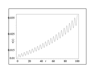
Figure 3: Evolution of the BI Universe with a bulk viscosity and a share viscosity. The volume scale $\tau$ in this case expands exponentially with a small oscillation.

As one sees from the Fig. 3 the exponential mode of evolution of the BI Universe is accompanied by an oscillation. The space-time singularity in this case arises at $t\to-\infty$. Note that the negative $\Lambda$ gives rise to the exponential growth while the oscillation in the model occurs due to the viscosity.

III Conclusion

The role of viscous fluid and $\Lambda$ term in the evolution of a homogeneous, anisotropic Universe given by a Bianchi type-I space-time is studied. It is shown that the $\Lambda$ term plays very important role in BI cosmology. In particular, in case of a bulk viscosity, it provides an everlasting process of evolution with $\Lambda$ being negative, whereas, for some positive values of $\Lambda$ the BI Universe admits an oscillatory mode of expansion. It is also shown that a oscillatory mode of expansion of the BI space-time can take place with a negative $\Lambda$ as well, though it is accompanied by an exponential mode. Oscillation in this case arises due to viscosity. In this report we only consider some special cases those provides exact solutions. For a better knowledge about the evolution, it is important to perform some qualitative analysis of the system (2.42). A detailed analysis of the system in question plus some numerical solutions will be presented soon elsewhere.

References

- (1) W. Misner, Nature 214, 40 (1967).
- (2) W. Misner, Astrophys. J. 151, 431 (1968).
- (3) S. Weinberg, Astrophys. J. 168, 175 (1972).
- (4) S. Weinberg, Gravitation and Cosmology (New York, Wiley, 1972).
- (5) P. Langacker, Phys. rep. 72, 185 (1981).
- (6) L. Waga, R.C. Falcan, and R. Chanda, Phys. Rev. D 33, 1839 (1986).
- (7) T. Pacher, J.A. Stein-Schabas, and M.S. Turner, Phys. Rev. D 36, 1603 (1987).
- (8) Alan Guth, Phys. Rev. D 23, 347 (1981).
- (9) G.L. Murphy, Phys. Rev. D 8, 4231 (1973).
- (10) N.O. Santos, R.S. Dias, and A. Banerjee, J. Math. Phys. 26, 876 (1985).
- (11) V.A. Belinski and I.M. Khalatnikov, Soviet Journal JETP 69, 401, (1975).
- (12) A. Banerjee, S.B. Duttachoudhury, and A.K. Sanyal, J. Math. Phys. 26, 3010 (1985).
- (13) W. Huang, J. Math. Phys. 31, 1456 (1990).
- (14) K. Desikan, Gen. Relativ. Gravit. 29, 435 (1997).
- (15) K.D. Krori and A. Mukherjee, Gen. Relativ. Gravit. 32, 1429 (2000).
- (16) L.P. Chimento, A.S. Jacubi, V. Mndez, and R. Maartens, Class. Quantum Grav. 14, 3363 (1997).
- (17) H. van Elst, P. Dunsby, and R. Tavakol, Gen. Relativ. Gravit. 27, 171 (1995).
- (18) V.R. Gavrilov, V.N. Melnikov, and R. Triay, Class. Quantum Grav. 14, 2203 (1997).
- (19) J.D. Barrow, Nuc. Phys. B 310, 743 (1988).
- (20) Bijan Saha, Phys. Rev. D 64, \htmladdnormallink123501http://www.jinr.ru/ bijan/my_papers/PRD23501.pdf (2001).
- (21) Bijan Saha, Phys. Rev. D 69, \htmladdnormallink124010http://www.jinr.ru/ bijan/my_papers/PRD24010.pdf (2004).
- (22) Bijan Saha, ”Nonlinear spinor field in Bianchi type-I Universe filled with viscous fluid: some special \htmladdnormallinksolutions”http://www.jinr.ru/ bijan/my_pdf/visnls.pdf (to appear in Romanian Report of Physics in 2005).
- (23) K.C. Jacobs, Astrophys. J. 153, 661 (1968).
- (24) K.A. Bronnikov and G.N. Shikin, Gravitation Cosmol. 7, 231 (2001).
- (25) S. Fay, Class. Quantum Grav. 17, 2663 (2000).
- (26) E. Kamke, Differentialgleichungen losungsmethoden und losungen (Akademische Verlagsgesellschaft, Leipzig, 1957).
- (27) A.P. Prudnikov, Yu.A. Brychkov, and O.I. Marichev, Integrals and series. v.1: Elementary functions (New York, Gordon and Breach, 1986).