High-Speed Cylindrical Collapse of Perfect Fluid

Abstract

The gravitational collapse of a cylindrically distributed perfect fluid is studied. We assume that the collapsing speed of the fluid is very large and investigate such a situation using recently proposed high-speed approximation scheme. We show that if the value of the pressure divided by the energy density is bounded below by some positive value, the high-speed collapse is necessarily decelerated by pressure repulsion so significantly that this approximation scheme becomes inapplicable. However, even in the case of a mono-atomic ideal gas, which is a typical example of the bounded case, an arbitrarily large tidal force for freely falling observers can be realized before the high-speed approximation breaks down if the initial collapsing velocity is set to a very large value. By contrast, in case that the equation of state is sufficiently soft, we find that the high-speed collapse is maintained until a spacetime singularity forms.

1 Introduction

Gravitational collapse is an important topics in general relativity. With recent observational studies of gravitational waves using laser interferometric detectors such as LIGO, TAMA, VIRGO and GEO[1, 2], the study of gravitational collapse as a source of gravitational radiation was gained its importance. Almost all theoretical studies on generation mechanisms of gravitational emissions have been proceeded under the assumption that the spacetime singularities are hidden inside black holes. However, if the spacetime singularities are not enclosed by event horizons, the situation could be completely different from the case with horizons. Such a spacetime singularity is called a globally naked singularity. Nakamura, Shibata and one of the present authors have conjectured that a large spacetime curvature in the neighborhood of a globally naked singularity can propagate away to infinity in the form of gravitational radiation due to the lack of an event horizon and therefore the mass of the naked singularity is lost through large gravitational emissions[3].

Here we should note the cosmic censorship conjecture[4]. The statement of the cosmic censorship is, roughly speaking, that a spacetime singularity formed as the result of physically reasonable initial data cannot be naked. In connection with this matter, recently, Harada and one of the present authors proposed the alternative concept of the spacetime singularity, called a ‘spacetime border’[10]. There is a cut-off energy scale $\Lambda$ above which general relativity cannot describe any physical process; for example, $\Lambda$ could be the Planck scale $E_{\rm pl}$ ($\sim 10^{19}$GeV), or it might be a scale on the order of several TeV in the brane world scenario[11, 12, 13, 14]. Thus, spacetime regions of energy scales higher than $\Lambda$ should be regarded as singularities for general relativity. This viewpoint leads to the definition of a spacetime border as follows. A spacetime border is defined as a region of the spacetime which satisfies the inequality

$$\inf_{\cal A}F\geq{\Lambda^{4}\over E_{\rm pl}^{2}}~{},$$ (1)

where the curvature strength $F$ is given for instance by

$$F:=\max(|R^{a}{}_{a}|,|R^{ab}R_{ab}|^{1/2},|R^{abcd}R_{abcd}|^{1/2},|R_{\mu\nu\rho\sigma}|).$$ (2)

Here we have extended the original definition of $F$ to a slightly more general one. In this case, $F$ includes components $R_{\mu\nu\rho\sigma}$ of the Riemann tensor with respect to the tetrad basis transported parallelly along timelike curves of bounded acceleration, i.e., the tidal force experienced by physically reasonable observers. In a practical sense, the visible border is a useful concept as an alternative to the naked singularity.

In the investigation of naked singularity formation, mainly spherically symmetric systems have been studied[15], because they are simple but possess rich physical content. However, in a sense, such a system is too simple, as there is no degree of gravitational radiation. Therefore, in order to study the generation mechanism of gravitational radiation, we have to add non-spherical perturbations to this system[5, 6, 7, 8, 9] or consider non-spherically symmetric spacetimes. In this sense, cylindrically symmetric gravitational collapse has significant physical meaning, because there is a degree of gravitational radiation, and, further, the spacetime singularity in this system is naked[16, 17]. There are a few numerical studies of gravitational wave generation through cylindrical gravitational collapse[18, 19, 20]. Although there has been debate about their results, the present authors have revealed with an analytic study that there is no inconsistency[21]. In any case, these investigations give strong evidence for the generation of a large amount of gravitational radiation through cylindrical gravitational collapse. There are also several studies concerning cylindrical gravitational collapse, and these have improved our understanding of non-spherical relativistic dynamics[22, 23, 24, 25, 26, 27].

In this paper, we investigate the gravitational collapse of a cylindrical, thick shell composed of a perfect fluid by generalizing a high-speed approximation for a cylindrical thick dust shell[21] to the case of non-vanishing pressure. In this approximation scheme, the collapsing speed is assumed to be almost equal to the speed of light. Therefore we treat the deviation of the 4-velocity of the perfect fluid from null as a small perturbation. By using this approximation scheme, we study the effect of the pressure in the case of a very large collapsing velocity.

This paper is organized as follows. In $\S$2, we briefly review the formulation of a spacetime with whole-cylinder symmetry[29]. Then in $\S$3, we present the high-speed approximation scheme for a general perfect fluid. In $\S$4, we discuss the effect of pressure and determine whether the pressure prevents high-speed collapse. Because an ideal mono-atomic gas behaves like radiation in the high energy limit, in $\S$5 we solve the Euler equation with a linear equation of state including the radiation case, and show that if the initial collapsing velocity is chosen appropriately, then an arbitrarily strong tidal force for freely falling observers is realized in the neighborhood of the symmetric axis of the cylinder before the high-speed approximation becomes inapplicable. Finally, $\S$6 is devoted to a summary and discussion.

In this paper, we adopt $c=1$ unit and basically follow the convention and notation in the textbook by Wald[30].

2 Cylindrically symmetric perfect fluid system

We focus on a spacetime of whole-cylinder symmetry. Such a system possesses the line element[28]

$$ds^{2}=e^{2(\gamma-\psi)}\left(-dt^{2}+dr^{2}\right)+e^{2\psi}dz^{2}+e^{-2\psi}R^{2}d\varphi^{2},$$ (3)

where the metric variables $\gamma$, $\psi$ and $R$ are functions of $t$ and $r$. Then, the Einstein equations are

$$\gamma^{\prime}=\left({R^{\prime}}^{2}-{\dot{R}}^{2}\right)^{-1}\biggl{\{}RR^{\prime}\left({\dot{\psi}}^{2}+{\psi^{\prime}}^{2}\right)-2R{\dot{R}}{\dot{\psi}}\psi^{\prime}+R^{\prime}R^{\prime\prime}-{\dot{R}}{\dot{R}}^{\prime}$$

$$~{}~{}~{}~{}-8\pi G\sqrt{-g}\left(R^{\prime}T^{t}{}_{t}+{\dot{R}}T^{r}{}_{t}\right)\biggr{\}},$$ (4)

$${\dot{\gamma}}=-\left({R^{\prime}}^{2}-{\dot{R}}^{2}\right)^{-1}\biggl{\{}R{\dot{R}}\left({\dot{\psi}}^{2}+{\psi^{\prime}}^{2}\right)-2RR^{\prime}{\dot{\psi}}\psi^{\prime}+{\dot{R}}R^{\prime\prime}-R^{\prime}{\dot{R}}^{\prime}$$

$$~{}~{}~{}~{}-8\pi G\sqrt{-g}\left({\dot{R}}T^{t}{}_{t}+R^{\prime}T^{r}{}_{t}\right)\biggr{\}},$$ (5)

$${\ddot{\gamma}}-\gamma^{\prime\prime}={\psi^{\prime}}^{2}-{\dot{\psi}}^{2}-{8\pi G\over R}\sqrt{-g}T^{\varphi}{}_{\varphi},$$ (6)

$${\ddot{R}}-R^{\prime\prime}=-8\pi G\sqrt{-g}\left(T^{t}{}_{t}+T^{r}{}_{r}\right),$$ (7)

$${\ddot{\psi}}+{{\dot{R}}\over R}{\dot{\psi}}-\psi^{\prime\prime}-{R^{\prime}\over R}\psi^{\prime}=-{4\pi G\over R}\sqrt{-g}\left(T^{t}{}_{t}+T^{r}{}_{r}-T^{z}{}_{z}+T^{\varphi}{}_{\varphi}\right),$$ (8)

where the dot represents differentiation with respect to $t$ and the prime that with respect to $r$.

In this paper, we consider a perfect fluid. The stress-energy tensor is written

$$T_{\mu\nu}=(\rho+p)u_{\mu}u_{\nu}+pg_{\mu\nu},$$ (9)

where $g_{\mu\nu}$ is the metric tensor, $\rho$ is the energy density, $p$ is the pressure, and $u^{\mu}$ is the 4-velocity of the fluid element. Due to the assumption of the whole-cylinder symmetry, the components of the 4-velocity $u^{\mu}$ are written

$$u^{\mu}=u^{t}\left(1,-1+V,~{}0,~{}0\right),$$ (10)

where $V$ should be positive so that $u^{\mu}$ is timelike. With the normalization $u^{\mu}u_{\mu}=-1$, $u^{t}$ is expressed as

$$u^{t}={e^{-\gamma+\psi}\over\sqrt{V\left(2-V\right)}}.$$ (11)

Here we introduce the new variables $D$ and $P$ defined by

$$D := {\sqrt{-g}(\rho+p)u^{t}\over\sqrt{V\left(2-V\right)}}={Re^{\gamma-\psi}(\rho+p)\over V\left(2-V\right)},$$ (12)

$$P := {Re^{\gamma-\psi}p\over V\left(2-V\right)},$$ (13)

where $g$ is the determinant of the metric tensor $g_{\mu\nu}$. The components of the stress-energy tensor $T^{\alpha}{}_{\beta}$ are then expressed as

$$\sqrt{-g}T^{t}{}_{t} = e^{\gamma-\psi}\left\{-D+V\left(2-V\right)P\right\},$$ (14)

$$\sqrt{-g}T^{r}{}_{t} = e^{\gamma-\psi}D(1-V)=-\sqrt{-g}T^{t}{}_{r},$$ (15)

$$\sqrt{-g}T^{r}{}_{r} = e^{\gamma-\psi}\left\{\left(1-V\right)^{2}D+V\left(2-V\right)P\right\},$$ (16)

$$\sqrt{-g}T^{z}{}_{z} = \sqrt{-g}T^{\varphi}{}_{\varphi}=e^{\gamma-\psi}V(2-V)P,$$ (17)

and the other components vanish.

The equation of motion $\nabla_{\alpha}T^{\alpha}{}_{\beta}=0$ leads to

$$\partial_{u}D = -{1\over 2}(DV)^{\prime}+{1\over 2}\left\{V(2-V)P\right\}{\dot{}}+{D\over 2}(1-V)\left\{2\partial_{u}(\psi-\gamma)-V({\dot{\psi}}-{\dot{\gamma}})\right\}$$ (18)

$$+ {1\over 2}PV(2-V)({\dot{\psi}}-{\dot{\gamma}}-{\dot{R}}/R),$$

$$D\partial_{u}V = (1-V)\partial_{u}D+{1\over 2}\left\{V(1-V)D-V(2-V)P\right\}^{\prime}$$ (19)

$$- {D\over 2}\left\{2\partial_{u}(\psi-\gamma)-V({\dot{\psi}}-{\dot{\gamma}})\right\}+{1\over 2}PV(2-V)(\gamma^{\prime}-\psi^{\prime}+R^{\prime}/R),$$

where $u=t-r$ is the retarded time and $\partial_{u}$ is the partial derivative of $u$ with fixed advanced time $v=t+r$. The first equation comes from the $t$-component, while the second one comes from the $r$-component. The $z$- and $\varphi$-components are trivial.

To estimate the energy flux of gravitational radiation, we adopt the $C$-energy $E$ and its flux vector proposed by Thorne[28]. The $C$-energy $E=E(t,r)$ is the energy per unit coordinate length along the $z$-direction within a radius $r$ at time $t$. It is defined by

$$E={1\over 8}\left\{1+e^{-2\gamma}\left({\dot{R}}^{2}-{R^{\prime}}^{2}\right)\right\}.$$ (20)

The energy flux vector $J^{\mu}$ associated with $C$-energy is defined by

$$\sqrt{-g}J^{\mu}=\left({\partial E\over\partial r},-{\partial E\over\partial t},0,0\right).$$ (21)

By definition, $J^{\mu}$ is divergence free. Using the equations of motion for the metric variables, we obtain the expression for the $C$-energy flux vector as

$$\sqrt{-g}J^{t} = {e^{-2\gamma}\over 8\pi G}\biggl{\{}RR^{\prime}({\dot{\psi}}^{2}+{\psi^{\prime}}^{2})-2R{\dot{R}}{\dot{\psi}}\psi^{\prime}-8\pi G\sqrt{-g}(R^{\prime}T^{t}{}_{t}+{\dot{R}}T^{r}{}_{t})\biggr{\}},$$ (22)

$$\sqrt{-g}J^{r} = {e^{-2\gamma}\over 8\pi G}\biggl{\{}R{\dot{R}}({\dot{\psi}}^{2}+{\psi^{\prime}}^{2})-2RR^{\prime}{\dot{\psi}}\psi^{\prime}-8\pi G\sqrt{-g}(R^{\prime}T^{r}{}_{t}-{\dot{R}}T^{r}{}_{r})\biggr{\}},$$ (23)

while the other components vanish.

3 High-speed approximation for a perfect fluid

Let us consider the ingoing null limit of the cylindrical perfect fluid. Using $D$ and $P$, the stress-energy tensor is written

$$T_{\mu\nu}={e^{3(\psi-\gamma)}\over R}\left\{Dk_{\mu}k_{\nu}+e^{2(\gamma-\psi)}V(2-V)Pg_{\mu\nu}\right\},$$ (24)

where

$$k^{\mu}=(1,-1+V,~{}0,~{}0).$$ (25)

The timelike vector $k^{\mu}$ becomes an ingoing null vector in the limit $V\rightarrow 0_{+}$. Hence, in this limit with $D$ and $P$ fixed, the stress-energy tensor is identical to that of collapsing null dust,

$$T_{\mu\nu}\longrightarrow{e^{3(\psi-\gamma)}D\over R}k_{\mu}k_{\nu},$$ (26)

where

$$k^{\mu}\longrightarrow(1,-1,~{}0,~{}0).$$ (27)

This implies that in the case of a very large collapsing velocity, i.e., for $0<V\ll 1$, the perfect fluid system is approximated well by a null dust system. For this reason, we treat the deviation $V$ of the 4-velocity from null as a perturbation and perform a linear perturbation analyses.

In the case of collapsing null dust, the solution is easily obtained as

$$\psi = 0,$$ (28)

$$\gamma = \gamma_{B}(v),$$ (29)

$$R = r,$$ (30)

$$8\pi GDe^{\gamma} = {d\gamma_{B}\over dv},$$ (31)

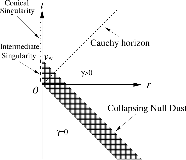
where $\gamma_{B}(v)$ is an arbitrary function of the advanced time $v$. This solution was obtained by Morgan[22] and was studied subsequently by Letelier and Wang[24] and Nolan[25] in detail. We regard this solution as a background spacetime for the perturbation analysis. The situation can be understood from Fig.1. The “density” $D$ is assumed to have compact support, $0<v<v_{\rm w}$, which is depicted by the shaded region. We find from Eqs.(26) and (30) that if $D$ does not vanish at the symmetric axis $r=0$, the components of the stress-energy tensor $T_{\mu\nu}$ with respect to the coordinate basis diverge there, and the same is true for the Ricci tensor by Einstein equations. This is a naked singularity which is depicted by the dashed line at $r=0$ on the interval $0<t<v_{\rm w}$ in Fig.1. Although all the scalar polynomials of the Riemann tensor vanish there, freely falling observers experience an infinite tidal force at $r=0$ for $0<t<v_{\rm w}$[24]. The short dashed line corresponding to $t=r$ represents the Cauchy horizon associated with this naked singularity. The region satisfying $t\geq v_{\rm w}$ at $r=0$ is a conical singularity which is depicted by the dotted line in Fig.1.

Figure 1: Morgan’s cylindrical null dust solution. Null dust exists in the shaded region. In this situation depicted, $D(v)>0$ for $0<v<v_{\rm w}$. The dashed line on the $t$-axis corresponds to the intermediate singularity at which an observer experiences an infinite tidal force, although the scalar polynomials of the Riemann tensor do not vanish. The dotted line on $t$-axis represents the conical singularity. The Cauchy horizon is represented by the short dashed line corresponding to $t=r$.

Now let us consider a general perfect fluid with very large collapsing velocity. To carry out the linear perturbation analysis, we introduce a small parameter $\epsilon$ and assume the orders $V=O(\epsilon)$ and $\psi=O(\epsilon)$. Further, we rewrite the variables $\gamma$, $R$ and $D$ as

$$e^{\gamma} = e^{\gamma_{B}}(1+\delta_{\gamma}),$$ (32)

$$R = r(1+\delta_{R}),$$ (33)

$$D = D_{B}(1+\delta_{D}),$$ (34)

and assume that $\delta_{\gamma}$, $\delta_{R}$ and $\delta_{D}$ are $O(\epsilon)$, where

$$D_{B}:={1\over 8\pi Ge^{\gamma_{B}}}{d\gamma_{B}\over dv}.$$ (35)

We call the perturbative analysis with respect to this small parameter $\epsilon$ the ‘high-speed approximation’.

The first-order equations with respect to $\epsilon$ are given as follows: the Einstein equations (4)$-$(8) lead to

$$\delta_{\gamma}{}^{\prime}=8\pi GD_{B}e^{\gamma_{B}}\left\{\delta_{\gamma}-\psi+\delta_{D}-2\partial_{v}(r\delta_{R})-2PV/D_{B}\right\}+(r\delta_{R})^{\prime\prime},$$ (36)

$${\dot{\delta}}_{\gamma}=8\pi GD_{B}e^{\gamma_{B}}\left\{\delta_{\gamma}-\psi+\delta_{D}-2\partial_{v}(r\delta_{R})-V\right\}+(r{\dot{\delta}_{R}})^{\prime},$$ (37)

$${\ddot{\delta}}_{\gamma}-\delta_{\gamma}{}^{\prime\prime}=-{16\pi G\over r}e^{\gamma_{B}}PV,$$ (38)

$$r{\ddot{\delta}}_{R}-(r\delta_{R})^{\prime\prime}=16\pi Ge^{\gamma_{B}}(D_{B}-2P)V,$$ (39)

$${\ddot{\psi}}-\psi^{\prime\prime}-{1\over r}\psi^{\prime}={8\pi G\over r}e^{\gamma_{B}}(D_{B}-2P)V;$$ (40)

the conservation law (18) leads to

$$\partial_{u}\left(\delta_{D}+\delta_{\gamma}-\psi\right) = -{1\over 2D_{B}}{dD_{B}\over dv}V-{1\over 2}\left(V^{\prime}-{d\gamma_{B}\over dv}V\right)$$ (41)

$$~{}~{}~{}~{}~{}~{}~{}~{}~{}~{}~{}~{}~{}~{}~{}~{}~{}~{}+{1\over D_{B}}\left\{(PV){\dot{}}-PV{d\gamma_{B}\over dv}\right\};$$

the Euler equation (19) becomes

$$\partial_{u}\left\{(D_{B}-2P)V\right\}={PV\over r},$$ (42)

where we have used Eq.(41).

The $C$-energy $E$ up to first order in $\epsilon$ is given by

$$E={1\over 8}\left[1-e^{-2\gamma_{B}}+2e^{-2\gamma_{B}}\left\{\delta_{\gamma}-\left(r\delta_{R}\right)^{\prime}\right\}\right].$$ (43)

We can easily see in Eq.(35) that $\gamma_{B}$ is constant in the vacuum region, $D_{B}=0$. Further, from Eqs.(36) and (37), we find that $\delta_{\gamma}-(r\delta_{R})^{\prime}$ is constant in the vacuum region. Therefore, up to first order, the $C$-energy is constant in the vacuum region. This means that in the vacuum region, the $C$-energy flux vector $J^{\mu}$ vanishes up to this order, and thus it is a second-order quantity given by

$$\sqrt{-g}J^{t} = {r\over 8\pi G}\left({\dot{\psi}}^{2}+{\psi^{\prime}}^{2}\right),$$ (44)

$$\sqrt{-g}J^{r} = -{r\over 4\pi G}{\dot{\psi}}\psi^{\prime}.$$ (45)

In this case, the $C$-energy flux vector takes a form very similar to that of the massless Klein-Gordon field.

4 Does pressure prevents the high-speed collapse?

Assuming that both the energy density $\rho$ and pressure $p$ of the fluid are positive, we introduce the quantity

$$c_{\rm s}(u,v)=\sqrt{p\over\rho}$$ (46)

If the dominant energy condition is satisfied, $c_{\rm s}$ is smaller than or equal to the speed of light[30]. However, in this paper, we assume a more stringent constraint on $c_{\rm s}$, namely

$$c_{\rm s}<1.$$ (47)

As shown below, the present approximation scheme cannot treat the case of $c_{\rm s}=1$.

From Eqs.(12) and (13) and by using Eq.(46), we obtain

$$P={c_{\rm s}{}^{2}\over 1+c_{\rm s}{}^{2}}D.$$ (48)

With the above equation, the Euler equation (42) can be rewritten as

$$\partial_{u}\ln\left({1-c_{\rm s}{}^{2}\over 1+c_{\rm s}{}^{2}}V\right)={c_{\rm s}{}^{2}\over(1-c_{\rm s}{}^{2})r}.$$ (49)

Integrating this equation formally, we obtain

$$V={1+c_{\rm s}{}^{2}\over 1-c_{\rm s}{}^{2}}\exp\left[\int^{u}_{U(v)}dx{2c_{\rm s}{}^{2}(x,v)\over\{1-c_{\rm s}{}^{2}(x,v)\}(v-x)}\right],$$ (50)

where $U(v)$ is an arbitrary function of the advanced time $v$. In the above equation, the velocity perturbation $V$ is not defined for $c_{\rm s}=1$, and thus the high-speed approximation is not applicable to this case.

We consider two cases, one in which $c_{\rm s}$ is bounded below by some positive constant, and one in which $c_{\rm s}$ vanishes in the large energy density limit, $\rho\rightarrow\infty$.

4.1 Bounded case

In case that $c_{\rm s}$ is bounded below by some positive value, we have the inequality

$${2c_{\rm s}{}^{2}\over 1-c_{\rm s}{}^{2}}\geq b^{2},$$ (51)

where $b$ is some non-vanishing constant. Then from Eq.(49), we obtain

$$\partial_{u}\ln\left({1-c_{\rm s}{}^{2}\over 1+c_{\rm s}{}^{2}}V\right)\geq{b^{2}\over v-u}.$$ (52)

Integrating the above inequality, we obtain

$$V\geq{\rm Const}\times r^{-b^{2}},$$ (53)

where ‘Const’ should be positive. We find in the above inequality that the velocity perturbation $V$ diverges when the fluid element approaches the symmetric axis, $r=0$. This implies that in this case, the high-speed collapse is necessarily decelerated so significantly that the high-speed approximation breaks down.

4.2 Vanishing case

If $c_{\rm s}$ vanishes in the limit of a high energy density, $\rho\rightarrow\infty$, the behavior of the perfect fluid can differ from the case of bounded $c_{\rm s}$. When the fluid elements approach the background singularity, i.e., $r=0$ in the region of non-vanishing $D_{B}$, the energy density will become larger and larger. Thus, in this case, the asymptotic behavior of $c_{\rm s}$ near the background singularity will be given by

$$c_{\rm s}{}^{2}(u,v)\sim C_{\rm s}{}^{2}(t)r^{q}=C_{\rm s}{}^{2}(v-r)r^{q}\sim C_{\rm s}{}^{2}(v)r^{q},$$ (54)

where $C_{\rm s}$ is some function, and $q$ is a positive constant. Substituting the above asymptotic form of $c_{\rm s}$ into Eq.(50), we obtain

$$V\sim C_{V}{}^{2}(v)\exp\left\{{2^{q+1}\over q}C_{\rm s}{}^{2}(v)r^{q}\right\},$$ (55)

where

$$C_{V}(v)=\exp\left[-{C_{\rm s}{}^{2}(v)\over q}\left\{v-U(v)\right\}^{q}\right].$$ (56)

Note that $C_{V}$ should have the same support as the background density variable $D_{B}$. Therefore, in this case, the velocity perturbation remains finite, even at the background singularity. This seems to imply that the naked singularity forms at the background singularity through this gravitational collapse. However, the full-order analysis is necessary to reach a definite conclusion.

Here, conversely, we consider the asymptotic equation of state that realizes the asymptotic behavior (54). We find from Eq.(12) that as the background singularity is approached, the energy density behaves as

$$\rho\sim{2VD_{B}\over re^{\gamma_{B}}}=({\rm function~{}~{}of}~{}~{}v)^{2}\times{1\over r},$$ (57)

where we have used the fact that $V$ becomes a function of the advanced time $v$ at $r=0$, as seen from Eq.(55). Therefore together with Eqs.(46) and (54), the above equation leads to

$$p=c_{\rm s}{}^{2}\rho\sim{\rm Const}\times\rho^{1-q}$$ (58)

near $r=0$, where ‘Const’ should be positive. This result suggests that a very soft equation of state is necessary so that the high-speed collapse is not halted by the pressure before spacetime singularity formation.

4.3 Generation of gravitational waves

Equation (40) implies that a larger velocity perturbation $V$ leads to a larger $|\psi|$. Because the $C$-energy flux in the asymptotically flat region is given by Eq.(45), this suggests a large gravitational emission by large $V$.

In the bounded $c_{\rm s}$ case, the growth of the velocity perturbation $V$ is unbounded as the background singularity is approached. Although a velocity perturbation $V$ larger than unity is meaningless in the present approximation scheme, this result suggests that a significant amount of gravitational radiation is generated by pressure deceleration near the background singularity. This is consistent with Piran’s numerical results, because Piran’s numerical simulations for a cylindrically distributed ideal gas show that a large amount of gravitational radiation is emitted when the pressure bounce occurs. However, here we stress that in this paper, we study the result for an arbitrarily large initial collapsing velocity of the fluid, while Piran’s numerical study is restricted to cases with momentarily static initial data.

In the case of vanishing $c_{\rm s}$, the velocity perturbation takes a finite value even at the background singularity. Therefore the situation here is similar to that for a dust fluid in the generation processes of gravitational waves[21].

5 Appearance of the spacetime border

When the gravitational collapse realizes a very high energy density, the fluid will behave as a mono-atomic ideal gas, due to the asymptotic freedom of the elementary interactions. Furthermore, the equation of state will be similar to that of the radiation, i.e., with $p=\rho/3$. This corresponds to the bounded $c_{\rm s}$ case, and the high-speed collapse is necessarily decelerated so significantly that the high-speed approximation becomes inapplicable before the fluid elements reach the background singularity. This result seems to imply that the formation of spacetime singularities is prevented by the occurrence of the pressure bounce. However, even if this is the case, as mentioned in $\S$1, it is physically important in a practical sense only whether the spacetime border forms before the occurrence of the pressure bounce. Therefore, here we consider the formation of the spacetime border in the bounded $c_{\rm s}$ case.

We consider a linear equation of state, i.e., $c_{\rm s}=$constant, which includes the case of radiation, $c_{\rm s}{}^{2}=1/3$. Using Eq.(48), the Euler equation (42) becomes

$$\partial_{u}V={2c_{\rm s}{}^{2}V\over\left(1-c_{\rm s}{}^{2}\right)(v-u)}.$$ (59)

As mentioned previously, the above equation is singular for stiff matter with $c_{\rm s}=1$. The case $c_{\rm s}=1$ corresponds to a massless Klein-Gordon field, and it is easy to see that no gravitational radiation is generated in the cylindrically symmetric case.

Equation (59) can be easily integrated, and we obtain

$$V=C_{L}(v)r^{-2c_{\rm s}{}^{2}/(1-c_{\rm s}{}^{2})},$$ (60)

where $C_{L}(v)$ is an arbitrary positive function of the advanced time $v$, and it should have the same support as the background density variable $D_{B}$. As discussed in the preceding section, $V$ diverges to $+\infty$ at the background singularity in the case that $0<c_{\rm s}<1$. This implies that the perturbation analysis necessarily breaks down in the neighborhood of the background singularity.

Once we know the velocity perturbation $V$, we can easily obtain solutions for $\delta_{\gamma}$, $\delta_{R}$ and $\psi$ from Eqs.(36)$-$(40) using the ordinary procedure to construct solutions of wave equations in flat spacetimes. We can also easily obtain a solution for $\delta_{D}$ by solving Eq.(41). However, in this paper, we do not construct the solutions for these variables but instead focus on the velocity perturbation $V$ only.

The high-speed approximation scheme is applicable only to situations in which $V\ll 1$. Therefore, Eq.(60) leads to a necessary condition for the applicability of high-speed approximation,

$$r\gg C_{L}{}^{(1-c_{\rm s}{}^{2})/2c_{\rm s}{}^{2}},$$ (61)

where $r$ is the radial position of a fluid element. It should be noted that if the arbitrary function $C_{L}$ is chosen sufficiently small, the present approximation scheme may be applicable even in the case of very small $r$. Because the tidal force experienced by freely falling observers diverges as the background singularity at $r=0$ is approached[24], the velocity perturbation $V$ remains sufficiently small for the case of an arbitrarily large tidal force for freely falling observers if $C_{L}$ is chosen sufficiently small. This implies that if the initial collapsing velocity is sufficiently large, the gravitational collapse of a cylindrically distributed perfect fluid with a linear equation of state forms a spacetime border. Because there is no event horizon in the present case, the spacetime border is necessarily visible. This result implies practically the violation of cosmic censorship.

6 Summary and discussion

In this paper, we have presented a high-speed approximation scheme applicable to a cylindrically symmetric perfect fluid. Within this approximation scheme, we have found that in the case of $c_{\rm s}$ bounded below by some positive value, the high-speed collapse of the perfect fluid is necessarily decelerated so significantly that the high-speed approximation becomes inapplicable. This result reveals the possibility of pressure bounces, because the deceleration of the collapsing velocity implies that the pressure repulsion overwhelms the gravitational attraction. If this expectation holds, then the spacetime singularity formation resulting from the adiabatic collapse of a cylindrical perfect fluid of a physically reasonable ideal gas is impossible. However, here we should note that if the initial collapsing velocity is very large, a spacetime border (i.e., a region with spacetime curvature so large that the quantum effects in gravity are important) is realized before the high-speed approximation scheme breaks down. Because a horizon does not form in the system considered here, the spacetime border is necessarily visible. Therefore, this result implies practically the violation of cosmic censorship. By contrast, in the case that $c_{\rm s}$ vanishes in the limit of high energy density, $\rho\rightarrow\infty$, the high-speed collapse continues until a naked singularity forms. Thus, it is likely that if the equation of state is sufficiently soft, so that $p$ is proportional to $\rho^{1-q}$ with $0<q<1$, high-speed collapse is not prevented by the effect of the pressure, and thus a naked singularity forms.

Equation (40) implies that a large velocity perturbation $V$ leads to the efficient generation of gravitational radiation. Therefore, the unlimited growth of $V$ in the bounded $c_{\rm s}$ case implies the generation of significant gravitational radiation. Contrastingly, in the case that $c_{\rm s}$ vanishes in the high energy density limit, $V$ is finite, even at the background singularity. In this case, the behavior of the perfect fluid will be similar to that of a dust fluid, in which case a thinner cylindrical shell generates the larger amount of gravitational radiation[21].

In the case that $c_{\rm s}$ vanishes in the high energy density limit, the gravitational emission from the naked singularity might have some physical importance. In the present approximation scheme, the metric variables are regarded as test fields in the background spacetime. Thus, if we appropriately impose boundary conditions on these variables at the background singularity, we can obtain solutions of the linearized Einstein equations and estimate the energy carried away by the gravitational waves from the naked singularity in this case. This topics will be discussed elsewhere.[31]

The approximation scheme used here is a kind of perturbation method. Strictly speaking, the full-order analysis is necessary to reach a definite conclusion, although the results up to first order might have significant physical meaning. Therefore, a higher-order analysis should be meaningful, but this is a future work.

References

- [1] C. Cutler and K. S. Thorne, in Proceedings of the 16th International Conference on General Relativity and Gravitation, edited by N.T. Bishop and S.D. Maharaj (World Scientific, 2002), p. 72.
-
[2]
H. Tagoshi et al., Phys. Rev D63 (2001), 062001.
M. Ando et al., Phys. Rev. Lett. 87 (2001), 3950. - [3] T. Nakamura, M. Shibata and K. Nakao, Prog. of Theor. Phys. 89 (1993), 821.
- [4] R. Penrose, Riv. Nuovo Cim. 1 (1969), 252.
- [5] H. Iguchi, T. Harada and K. Nakao, Phys. Rev. D57 (1998), 7262.
- [6] H. Iguchi, T. Harada and K. Nakao, Prog. Theor. Phys. 101 (1999), 1235.
- [7] H. Iguchi, T. Harada and K. Nakao, Prog. Theor. Phys. 103 (2000), 53.
- [8] K. Nakao, H. Iguchi and T. Harada, Phys. Rev. D63 (2001), 084003.
- [9] T. Harada, H. Iguchi and K. Nakao, Prog. Theor. Phys. 107 (2002), 449.
- [10] T. Harada and K. Nakao, Phys. Rev. D70 (2004), 041501.
- [11] N. Arkani-Hamed, S. Dimopoulos and G. Dvali, Phys. Lett. B429 (1998), 263.
- [12] I. Antoniadis, N. Arkani-Hamed, S. Dimopoulos and G. Dvali, Phys. Lett. B436 (1998), 257.
- [13] L. Randall and R. Sundrum, Phys. Rev. Lett. 83 (1999), 3370.
- [14] L. Randall and R. Sundrum, Phys. Rev. Lett. 83 (1999), 4690.
- [15] P. Joshi, Global Aspects in Gravitation and Cosmology, (Oxford University Press, 1993).
- [16] K.S. Thorne, in Magic Without Magic; John Archibald Wheeler, edited by J. Klauder (Frieman, San Francisco, 1972), p231.
- [17] S. A. Hayward, Class. Quantum Grav. 17 (2000), 1749.
- [18] T. Piran, Phys. Rev. Lett. 41 (1978), 1085.
- [19] F. Echeverria, Phys. Rev. D47 (1993), 2271.
- [20] T. Chiba, Prog. Theor. Phys. 95 (1996), 321.
- [21] K. Nakao and Y. Morisawa, Class. Quantum Grav. 21 (2004), 2101.
- [22] T. A. Morgan, Gen. Relat. Gravit. 4 (1973) 273.
- [23] T. Apostolatos and K.S. Thorne, Phys. Rev. D46 (1992), 2435.
- [24] P. S. Letelier and A. Wang, Phys. Rev. D49 (1994), 5105.
- [25] B.C. Nolan, Phys. Rev. D65 (2002), 104006.
- [26] P. R. C. T. Pereira and A. Wang, Phys. Rev. D62 (2000), 124001.
- [27] B.C. Nolan and L.V. Nolan, Calss. Quantum Grav. 21 (2004), 3693.
- [28] K.S. Thorne, Phys. Rev. 138 (1965), B251.
- [29] M.A. Melvin, Phys. Lett. 8 (1964), 65; Phys. Rev. 139 (1965), B225.
- [30] R. M. Wald, General Relativity (The University of Chicago Press, 1984).
- [31] K. Nakao and Y. Morisawa, in preparation.