Clock rate comparison in a uniform gravitational field

Abstract

A partially alternative derivation of the expression for the time dilation effect in a uniform static gravitational field is obtained by means of a thought experiment in which rates of clocks at rest at different heights are compared using as reference a clock bound to a free falling reference system (FFRS). Derivations along these lines have already been proposed, but generally introducing some shortcut in order to make the presentation elementary. The treatment is here exact: the clocks whose rates one wishes to compare are let to describe their world lines (Rindler’s hyperbolae) with respect to the FFRS, and the result is obtained by comparing their lengths in space-time. The exercise may nonetheless prove pedagogically instructive insofar as it shows that the exact result of General Relativity (GR) can be obtained in terms of physical and geometrical reasoning without having recourse to the general formalism. Only at the end of the paper the corresponding GR metric is derived, to the purpose of making a comparison to the solutions of Einstein field equation. This paper also compels to deal with a few subtle points inherent in the very foundations of GR.

I Introduction

It is possible to show that the GR redshift formula for a uniform gravitational field

$$\frac{\Delta\nu}{\nu}=\frac{gh}{c^{2}},$$ (1)

it is an exact consequence of the EP, and its derivation does not require GR formalism price . As is well known, formula (1) was experimentally verified for the first time in 1960 by Pound and Rebka pound .

GR is a well-established theory, but it very often happens that its application to some specific case involves subtle points on which the agreement is not general: as a result, the conclusions of the analysis reported are often not univocal. This is the case, in particular, for the object of the present article, namely redshift in a uniform gravitational field.

In Weinberg’s treatise wein , for instance, the gravitational redshift effect is thus commented: ‘For a uniform gravitational field, this result could be derived directly from the Principle of Equivalence, without introducing a metric or affine connection’.

We have in fact already recalled that such derivations are possible and in an exact way price . Independently of this conclusion, one may always introduce transformations between reference frames at rest with respect to the matter generating the field and FFRS which, in the case of a uniform field, can become extended, or global. The most natural way to describe such a transformation are Rindler hyperbolae. But Rindler himself rindler , at the end of the paragraph of his book in which they are introduced and analysed, and after discussing the fact that SR can deal in a proper way with accelerated frames, states: ‘A uniform gravitational field can not be constructed by this method’. About 15 years ago, E.A. Desloge des1 ; des2 ; des3 ; des4 , in a sequence of four articles, carried out a systematic investigation on uniformly accelerated frames and on their connection with gravitation. In agreement with Rindler’s statement Desloge concludes that there is no exact equivalence between FFRF and uniform gravitational fields des3 ; des4 . By contrast, only three years later on this journal, E. Fabri fabri derived the expression of the time delay in a uniform gravitational field by explicit use of a FFRF, from which the world lines of objects at rest with the masses that generate the field are seen as Rindler hyperbolae. As far I know, Fabri’s paper is still the only one approaching the problem in this way.

In order to see whether a reconciliation between these apparently conflicting views could be obtained, I tried to set up an ideal experiment in which the rates of two standard clocks sitting at different heights in a uniform and static gravitational field are compared. I analysed in detail the measuring process as seen from a FFRF, chosen in the only way that does not lead to physical contradictions. The choice of the FFRF and the final results are in agreement with Fabri’s.

II Free-falling reference systems

EP is the basic idea from which the bulk of GR theory was developed. In our applications we will not deal with charged bodies and with non-gravitational forces in general. We are therefore entitled to overlook differences between weak and strong EP, differences that are present only when non-gravitational interactions are considered. We just consider the EP in this form:

A body in free fall does not feel any acceleration, and behaves locally as an inertial reference system of SR.

We know that physical gravitational fields are not uniform, and there always exist tidal forces that oblige to consider the validity of the EP only locally in space and time. The ideal case of a uniform and static field is however worth considering for its conceptual interest. In this ideal case FFRS, which in strictly physical situations are local inertial systems, would become non-local.

EP invites to consider FFR systems the proper inertial systems. Let us then try to build a non-local FFRF, denoted as $K$, in a 2-dimensional space-time universe and study the world line of a particle at rest with the masses that generate a uniform gravitational field $g$. Since this world line is considered with respect to the FFRF, we will associate to the particle a (local) frame $\Sigma^{-}$. It is easily proved rindler that the world line of a body falling along the vertical direction $x$ with constant proper acceleration $g$ is described by the hyperbola of equation:

$$x^{2}-c^{2}t^{2}=\frac{c^{4}}{g^{2}}.$$ (2)

Since we are considering acceleration with respect to $K$, it is material points at rest in $\Sigma^{-}$ that will describe an hyperbola of Eq. (2) in the Minkowski space-time of $K$ (with an acceleration pointing in the direction opposite to gravity). At $t=0$ an observer sitting in the FFRF and one at rest with the source of the gravitational field (sitting in $\Sigma$) have the same instantaneus rest frame and measure the same acceleration value (the first observer by observation of $\Sigma$’s trajectories, the second one measuring the force acting on him). On the other hand, an observer sitting $\Sigma^{-}$ will see material points at rest in $K$ describe more complicated world lines. They have been explicitly calculated hamilton , and turn out indeed to be very different from those described by Eq. (2) (on the same subject see ror ). Fortunately we do not need to deal with them in order to solve our problem.
In the following $x$ will be called ‘coordinate position’ and $t$ ‘coordinate time’, in order to distinguish them from proper coordinate and proper time measured by $\Sigma^{-}$. As usual $c$ is the speed of light, but for sake of simplicity in the following we will adopt units with $c=1$.

The space coordinate at time $0$ is $x_{0}=1/g$, so that Eq. (2) becomes

$$x^{2}-t^{2}=x_{0}^{2}.$$ (3)

A second RF $\Sigma^{+}$ which, at $t=0$, lies higher than $x_{o}$ by the amount $h$ as measured by $K$ is described by the following hyperbola

$$x^{2}-t^{2}={(x_{0}+h)}^{2},$$ (4)

where now gravitational acceleration depends on the coordinate. Because of this dependence we introduce the following notations:

$$g^{+}=\frac{1}{x_{0}+h}\qquad\qquad g^{-}=\frac{1}{x_{0}}.$$ (5)

The fact that the acceleration depends on the coordinate value, seems to be in contradiction with the uniformity of the field. We will discuss this problem in section IV where we shall see that our choice is the only possible one. In this section, we shall prove that adopting Eq. (3) and Eq. (4), three important physical conditions are satisfied:

• Local acceleration does not depend on time;

• The ratio between proper time intervals at different altitudes is also constant in time (possibly depending on the frames altitude), otherwise a Pound and Rebka-like experiment would give every day a different result;

• Radar distance between two observers situated at a different height is a constant quantity which is time independent (it will as well possibly depend on the altitude).

Properties (1), (2) and (3) are all experimentally verified. Property (1) is surely satisfied because it is the basis for deriving Rindler motion equation rindler . In section II.1 and II.2 we will prove also property (2) and (3) All this properties were already proven by desloge des2 , for the case of uniformly accelerated frames. We will prove this properties by a direct calculation that seems to be more intuitive and easy to understand.

II.1 Proper time intervals

We need to calculate the proper time interval along a world line between two generic coordinate times $t_{1}$ and $t_{2}$:

$$\tau_{12}=\int_{t_{1}}^{t_{2}}\sqrt{1-V^{2}}dt,$$ (6)

where $V$ it is the coordinate velocity in units with $c=1$. Differentiating Eq. (3) or Eq. (4) one obtains $V=t/x$ and using Eq. (3) and Eq. (4) in order to eliminate $x$, we can calculate the proper time interval $\tau^{-}$ along the lower and $\tau^{+}$ along the upper hyperbola

$$\tau^{-}_{12}=\int_{t_{1}^{-}}^{t_{2}^{-}}\frac{1}{\sqrt{1+(\frac{t}{x_{0}})^{2}}}dt=x_{0}\int_{\frac{t_{1}^{-}}{x_{0}}}^{\frac{t_{2}^{-}}{x_{0}}}\frac{1}{\sqrt{1+y^{2}}}dy$$ (7)

$$\tau^{+}_{12}=\int_{t_{1}^{+}}^{t_{2}^{+}}\frac{1}{\sqrt{1+(\frac{t}{x_{0}+h})^{2}}}dt=(x_{0}+h)\int_{\frac{t_{1}^{+}}{x_{0}+h}}^{\frac{t_{2}^{+}}{x_{0}+h}}\frac{1}{\sqrt{1+y^{2}}}dy.$$ (8)

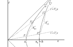
Figure 1: Proper times in $\Sigma^{+}$ and $\Sigma^{-}$

Considering the intersection of the two hyperbolae with two lines of constant coordinate velocity (see Fig. 1)

$$t=V_{1}x\qquad t=V_{2}x\qquad\qquad|V_{1}|,|V_{2}|<1,$$ (9)

one obtains two couples of points $P=P(x,t)$ in the Minkowski diagram, whose coordinates are:

$$P_{1}^{-}=\frac{\gamma_{1}}{g^{-}}\big{(}1,V_{1}\big{)}\quad P_{1}^{+}=\frac{\gamma_{1}}{g^{+}}\big{(}1,V_{1}\big{)}$$ (10)

$$P_{2}^{-}=\frac{\gamma_{2}}{g^{-}}\big{(}1,V_{2}\big{)}\quad P_{2}^{+}=\frac{\gamma_{2}}{g^{+}}\big{(}1,V_{2}\big{)},$$ (11)

where we have introduced the usual notation $\gamma=1/\sqrt{1-V^{2}}$. Coordinates of $P^{-}$ and $P^{+}$ are in simple proportions, and we have in particular

$$\frac{t_{1}^{+}}{t_{1}^{-}}=\frac{t_{2}^{+}}{t_{2}^{-}}=\frac{g^{-}}{g^{+}}=\frac{x_{0}+h}{x_{0}},$$ (12)

that proves the equality of integration extremes defining $\tau_{12}^{+}$ and $\tau_{12}^{-}$. Dividing Eq. (8) by Eq. (7), one finds:

$$\frac{\tau_{12}^{+}}{\tau_{12}^{-}}=\frac{g^{-}}{g^{+}}=\frac{x_{0}+h}{x_{0}},$$ (13)

so that one can conclude that:

Proper times intervals along two Rindler hyperbolae which are seen under the same angle centered in the origin are in a fixed proportion.

Considering as simultaneous all events laying on straight lines through the origin, the above statement proves property (2). This simultaneity will be proven in the next section.

Considering that $x_{0}=1/g^{-}$, Eq. (13) can also be recast in the following form:

$$\frac{\Delta\tau}{\tau}=\frac{\tau_{12}^{+}-\tau_{12}^{-}}{\tau^{-}_{12}}=g^{-}h.$$ (14)

II.2 Radar distance and light signals between Rindler hyperbolae

Let us draw a generic line through the origin in Minkowski space, which identifies points having the same coordinate velocity:

$$t=Vx\qquad\qquad|V|<1.$$ (15)

Intersecting this line with the low and upper hyperbolas identifies the points

$$P_{V}^{-}=\frac{\gamma}{g^{-}}\big{(}1,V\big{)};\qquad\quad P_{V}^{+}=\frac{\gamma}{g^{+}}\big{(}1,V\big{)}.$$ (16)

The equations of light rays departing from $P_{V}^{-}$ and $P_{V}^{+}$ are respectively

$$t=x-\gamma\frac{1-V}{g^{-}};\qquad t=-x+\gamma\frac{1+V}{g^{+}}.$$ (17)

Solving the system together with the Hyperbola equations (3) and (4)

$$\begin{cases}&t=x-\gamma\frac{1-V}{g^{-}}\\[5.0pt] &x^{2}-t^{2}=\frac{1}{(g^{+})^{2}}\end{cases}\hskip 56.9055pt\begin{cases}&t=-x+\gamma\frac{1+V}{g^{+}}\\[5.0pt] &x^{2}-t^{2}=\frac{1}{(g^{-})^{2}}\end{cases},$$ (18)

leads to the following intersection points:

$$P_{2}^{-}\!\!=\!\!\frac{\gamma g^{+}}{2}\!\Big{(}\!\frac{1+V}{(g^{+})^{2}}\!+\!\frac{1-V}{(g^{-})^{2}},\frac{1+V}{(g^{+})^{2}}\!-\!\frac{1-V}{(g^{-})^{2}}\!\Big{)};\quad P^{+}_{2}\!\!=\!\!\frac{\gamma g^{-}}{2}\!\Big{(}\!\frac{1+V}{(g^{+})^{2}}\!+\!\frac{1-V}{(g^{-})^{2}},\frac{1+V}{(g^{+})^{2}}\!-\!\frac{1-V}{(g^{-})^{2}}\!\Big{)}.$$ (19)

In the same way it is possible to calculate intersection points between the two hyperbolas and the incoming light rays:

$$P_{1}^{-}\!\!=\!\!\frac{\gamma g^{+}}{2}\!\Big{(}\!\frac{1+V}{(g^{-})^{2}}\!+\!\frac{1-V}{(g^{+})^{2}},\frac{1+V}{(g^{-})^{2}}\!-\!\frac{1-V}{(g^{+})^{2}}\!\Big{)};\quad P^{+}_{1}\!\!=\!\!\frac{\gamma g^{-}}{2}\!\Big{(}\!\frac{1+V}{(g^{-})^{2}}\!+\!\frac{1-V}{(g^{+})^{2}}^{\prime}\frac{1+V}{(g^{-})^{2}}\!-\!\frac{1-V}{(g^{+})^{2}}\!\Big{)}.$$ (20)

For any value of $V$, we have the following proportions

$$\frac{x_{1}^{+}}{x_{1}^{-}}=\frac{x_{2}^{+}}{x_{2}^{-}}=\frac{t_{1}^{+}}{t_{1}^{-}}=\frac{t_{2}^{+}}{t_{2}^{-}}=\frac{g^{-}}{g^{+}}=\frac{x_{0}+h}{x_{0}},$$ (21)

from which one see that $P_{1}^{-}$ is aligned with $P^{+}_{1}$, and $P_{2}^{-}$ is aligned with $P^{+}_{2}$ (as showed in Fig. 2).

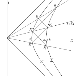
Figure 2: Light signal between two hyperbolae

We have thus found the following result which, as far as we know, was not previously pointed out:

Light rays through a couple of events with the same coordinate velocity laying on a Rindler hyperbola, intersect other Rindler hyperbolae in a couple of points that have in turn the same coordinate velocity.

This property it is an extra bonus, as we did not request it in our premise at the beginning of section II, and it will make it easier to perform clock rate comparison in an operational way. As a result of the above calculations, it is clear that observers in $\Sigma^{-}$ and in $\Sigma^{+}$ will consider simultaneous all the events laying on straight lines through the origin of the Minkowski diagram. With this definition of simultaneity we can calculate the proper time $\tau_{S}^{-}$ elapsed in $\Sigma^{-}$ when a light ray covers the distance necessary to go from $\Sigma^{-}$ to $\Sigma^{+}$ and the proper time taken for the return trip:

$$\tau_{S}^{-}=\int_{t^{-}_{V}}^{t^{-}_{2}}\frac{1}{\sqrt{1+(\frac{t}{x_{0}})^{2}}}dt=x_{0}\int_{\frac{t^{-}_{V}}{x_{0}}}^{\frac{t^{-}_{2}}{x_{0}}}\frac{1}{\sqrt{1+y^{2}}}dy$$ (22)

$$\tau_{R}^{-}=\int_{t^{-}_{1}}^{t^{-}_{V}}\frac{1}{\sqrt{1+(\frac{t}{x_{0}})^{2}}}dt=x_{0}\int_{\frac{t^{-}_{1}}{x_{0}}}^{\frac{t^{-}_{V}}{x_{0}}}\frac{1}{\sqrt{1+y^{2}}}dy.$$ (23)

The calculation leads to constant quantities

$$\tau_{S}^{-}=\tau_{R}^{-}=x_{0}\ln{\frac{x_{0}+h}{x_{0}}}=\frac{1}{g^{-}}\ln{\frac{g^{-}}{g^{+}}}.$$ (24)

Calculation of proper times relative to an observer at rest with $\Sigma^{+}$ leads also to an equal and constant time, whose value is in this case:

$$\tau^{+}_{S}=\tau^{+}_{R}=(x_{0}+h)\ln{\frac{x_{0}+h}{x_{0}}}.$$ (25)

This is in our view an important result, which, together with our new notion of simultaneity between $\Sigma^{-}$ and $\Sigma^{+}$ proves the following statement:

The proper time, as measured by an observer on a Rindler hyperbola, taken by a light pulse to reach another Rindler Hyperbola is equal to the proper time taken for the return trip, and this proper time is constant.

With the proof of this property, we completely fulfilled request (3) of section II.

III Measurements

III.1 Clock delay

All necessary physical requirements having thus been satisfied, we feel entitled to set up a thought experiment in which two identically constructed clocks sit at rest, in a uniform and static gravitational field, at fixed distances along a field line of force. As has become customary, we will give a name to the physicists involved in the measuring processes; let’s say that Alice enjoys her life staying at rest with $\Sigma^{-}$ and Bob staying higher in $\Sigma^{+}$. They will perform a measure in the following way (see Fig. 3):

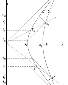
Figure 3: Alice and Bob compare their clock rate

a)

at time $t_{S1}$ Alice sends a light signal upwards;

b)

at time $t^{+}_{1}$ Alice’s light pulse is received by Bob. When Bob receives the signal he starts his clock and immediately sends back downwards a return light signal;

c)

at time $t_{R1}$ Alice receives the return signal from Bob. Adopting Einstein clock synchronization, she will argue that Bob clock started at the intermediate time between sending and receiving the light pulse. According to her clock this time is $\tau_{1}^{-}=\frac{\tau_{S1}^{-}+\tau_{R1}^{-}}{2}$, and corresponds to coordinate time $t_{1}$. In the previous section we saw that, with respect to the origin, this event is aligned with the event in which Bob started his clock;

d)

at time $t_{S2}$ Alice sends a light signal upwards;

e)

at time $t^{+}_{2}$ Alice light pulse is received by Bob. When Bob receives the signal he stops his clock and immediately sends back to Alice a return signal, in which the information of the proper time elapsed in Bob’s clock is stored;

f)

at time $t_{R2}$ Alice receives the return signal from Bob. She will argue that Bob clock had stopped at the intermediate time between sending and receiving the light pulse. According to her clock this time is $\tau_{2}^{-}=\frac{\tau_{S2}^{-}+\tau_{R2}^{-}}{2}$ which correspond to coordinate time $t_{2}$. We have again that in the Minkowski space-time of $K$, this event is aligned with the origin and the event in which Bob stopped his clock.

The necessary measurements have thus been done, and Alice can compare her time with Bob’s. It is immediately seen that any dependence on starting and stopping times cancels out, and that she will be able to compare two proper times seen under the same angle centered in the origin: $\tau^{-}_{12}=\tau^{-}_{2}-\tau^{-}_{1}$; $\tau^{+}_{12}=\tau^{+}_{2}-\tau^{+}_{1}$. These proper times satisfy Eq. (13) and Alice concludes  that

$$\frac{\Delta\tau}{\tau}=\frac{\tau^{+}_{12}-\tau^{-}_{12}}{\tau^{-}_{12}}=g^{-}{h}.$$ (26)

It is also possible to compare Bob’s proper time $\tau^{+}_{12}$ with Alice’s calculated either between the two emission or reception events. This would not make any difference, because in both cases we would have only added to and then subtracted from $\tau^{-}_{12}$ the same quantity (the times taken by the outward and return trips given by $\tau_{S}^{-}=\tau_{R}^{-}=x_{0}\ln{\frac{x_{0}+h}{x_{0}}}$).

III.2 Space dilation

In Eq. (24) and Eq. (25) we calculated the proper time elapsed in $\Sigma^{-}$ and $\Sigma^{+}$ for sending and receiving a light ray. Multiplying this time by the speed of light ($c=1$ in our units) we have radar distances $h^{-}$ (measured by $\Sigma^{-}$) and $h^{+}$ (measured by $\Sigma^{+}$)

$$h^{-}=x_{0}\ln{\frac{x_{0}+h}{x_{0}}};\qquad h^{+}=(x_{0}+h)\ln{\frac{x_{0}+h}{x_{0}}},$$ (27)

whose ratio give the following expression analog to time dilation:

$$\frac{h^{+}}{h^{-}}=\frac{x_{0}+h}{x_{0}}=\frac{g^{-}}{g_{+}}.$$ (28)

Keeping in mind that $x_{0}=1/g^{-}$ and $x_{0}+h=1/g^{+}$, solving Eq. (27) for $h$ one gets

$$h=x_{0}(e^{g^{-}h^{-}}-1)=x_{0}(e^{g^{+}h^{+}}-1),$$ (29)

which makes it possible to rewrite the time dilation formula using local coordinates:

$$\frac{\tau^{+}}{\tau^{-}}=1+g^{-}h=e^{g^{-}h^{-}}=e^{g^{+}h^{+}}.$$ (30)

One can prove that Eq. (30) is consistent with the following general result of GR rindler2 ,

$$\frac{\nu^{+}}{\nu^{-}}=e^{\phi(x_{0}+h)-\phi(x_{0})},$$ (31)

which expresses the redshift in terms of the Newtonian potential $\phi$ of the gravitational field. Indeed, calculating the potential difference we find:

$$\phi(x_{0}+h)-\phi(x_{0})=\int_{x_{0}}^{x_{0}+h}g(x)dx=\ln\frac{x_{0}+h}{x_{0}}=\ln(1+g^{-}h)$$ (32)

which, inserted in Eq. (31), reproduces our time dilation formula (30).

A different expression was obtained by Desloge des4 who considered Eq. (30) valid only for a uniform accelerated frame. For uniform gravity fields, Desloge proves the following expression

$$\frac{\nu^{+}}{\nu^{-}}=e^{gh},$$ (33)

where gravitational acceleration is the same for top and bottom observers and the distance is measured from a FFRF. Eq. (33) is also consistent with Eq. (31), but its derivation is based on a particular metric:

$$ds^{2}=e^{2gh}dt^{2}-dh^{2},$$ (34)

whose exact determination involves solving Einstein’s field equation rindler3 , and does not lead to a uniquely defined result ror . We will show in section V that the metric of Eq. (34) is correct but the distance coordinate must be interpreted as radar distance measured from an observer at rest with the field.

For a better understanding of space dilation it is useful to calculate the infinitesimal distance measured with radar methods by two observers at rest with the field at different heights. We will use $dh^{-}_{x}$ for denoting radar measurements of an infinitesimal length located at coordinate $x$, performed by an observer in $\Sigma^{-}$, and $dh^{+}_{x}$ if the observer is located at $\Sigma^{+}$. A straightforward calculation, at first order, gives:

$$dh^{-}_{x}=x_{0}\bigg{(}\ln{\frac{x+dh}{x_{0}}}-\ln{\frac{x}{x_{0}}}\bigg{)}\approx\frac{x_{0}}{x}dh$$ (35)

$$dh^{+}_{x}=(x_{0}+h)\bigg{(}\ln{\frac{x+dh}{x_{0}}}-\ln{\frac{x}{x_{0}}}\bigg{)}\approx\frac{x_{0}+h}{x}dh,$$ (36)

whose ratio is:

$$\frac{dh^{+}_{x}}{dh^{-}_{x}}=\frac{x_{0}+h}{x_{0}}=\frac{g^{-}}{g^{+}}.$$ (37)

An important consequence of Eq. (37) is that $\Sigma^{-}$ and $\Sigma^{+}$ measure the same infinitesimal work per unit mass:

$$d\phi=g^{+}dh^{+}=g^{-}dh^{-}.$$ (38)

III.3 Gravitational acceleration

In this subsection, we want to compare physical measurements performed by different observers in the same local frame. Let us consider two different measurements in Bob’s frame ($\Sigma^{+}$):

1

Bob ($\Sigma^{+}$) performs direct measurements with clocks and rods built in $\Sigma^{-}$ (or built in $\Sigma^{+}$ but with the very same physical procedure as those used in $\Sigma^{-}$)

2

Alice ($\Sigma^{-}$) observes Bob’s frame by sending and receiving reflected light pulses.

The two measurements are in the following relations

$$\underbrace{dh_{x_{0}+h}^{-}}_{Alice^{\prime}s~{}measure}=\frac{g^{+}}{g^{-}}\underbrace{dh_{x_{0}+h}^{+}}_{Bob^{\prime}s~{}measure};\qquad\quad\underbrace{d\tau_{x_{0}+h}^{-}}_{Alice^{\prime}s~{}measure}=\frac{g^{+}}{g^{-}}\underbrace{d\tau_{x_{0}+h}^{+}}_{Bob^{\prime}s~{}measure}.$$ (39)

Therefore, for the same couple of events, Alice obtains the same average velocity measured by Bob, but measuring shorter space and time intervals. Because of these contractions, it easy to prove that Alice will measure larger accelerations than those measured by Bob:

$$\underbrace{g_{x_{0}+h}}_{Alice^{\prime}s~{}measure}=\frac{g^{-}}{g^{+}}\underbrace{g_{x_{0}+h}}_{Bob^{\prime}s~{}measure}.$$ (40)

We know that the value of the gravitational acceleration obtained by Bob is $g^{+}$ and, from Eq. (40), we learn that Alice will find that the gravitational acceleration in Bob’s frame is $g^{-}$. It easy to conclude that every observer sitting at rest with the source of gravity finds that the gravitational acceleration has the same value everywhere. The disagreement between observers sitting at a different height can be interpreted as a consequence of local space-time dilation.

It worthwhile to note also that, moving along $x$ direction in an infinite uniform field, the local gravitational acceleration will assume every possible value. This has an important consequence:

All infinite extended uniform gravitational fields are equivalent.

This seems a strange conclusion, but remember that our starting point was purely ideal, and we did not analysed whether and how such a field could be realized in the real world.

IV Falling frame choice

In this section I will discuss our FFRF choice, concluding that it is well motivated and indeed the only possible one.

After the identification of $\Sigma^{-}$ with the Rindler hyperbola $x^{2}-t^{2}=x_{0}^{2}$ (equation (3) in section II), we could try to identify $\Sigma^{+}$ with a spatial translation of Eq. (3):

$$(x-h)^{2}-t^{2}=x_{0}^{2}.$$ (41)

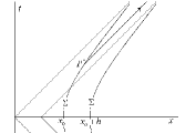
Figure 4: Light ray emitted from $\Sigma^{-}$ in $P^{*}$ will never reach $\Sigma^{+}$

This choice would warrant the very same gravitational acceleration in $\Sigma^{-}$ and $\Sigma^{+}$, but it gives rise to serious problems. The most evident one is illustrated in Fig. 4, where a situation is exhibited in which $\Sigma^{-}$ cannot send a light signal that reach $\Sigma^{+}$. More generally it is possible to prove, also graphically, that the hyperbola $x^{2}-t^{2}=(x_{0}+h)^{2}$ (equation (4) of section II) is the only one having constant radar distance from $\Sigma^{-}$.

Another important physical feature verified with our choice, is Lorentz invariance. For proving it, let us apply a boost $\Lambda$ of velocity $v=arcth\theta$ along $x$ direction to the hyperbola parametric equation rindler ; misner ; mould describing $\Sigma^{-}$

$$\mathbf{\Lambda}=\left(\begin{array}[]{ccc}\cosh\theta&-\sinh\theta\\[5.0pt] -\sinh\theta&\cosh\theta\end{array}\right)\hskip 56.9055pt\begin{cases}&x=x_{0}\cosh g\tau\\ &t=x_{0}\sinh g\tau\end{cases}.$$ (44)

The trasformed Hyperbola

$$\begin{cases}&x^{\prime}=x_{0}\cosh(g\tau-\theta)\\ &t^{\prime}=x_{0}\sinh(g\tau-\theta)\end{cases},$$ (45)

shows that the only effect of a Lorentz boost is a shift in the proper time origin $\Delta\tau=-\theta/g$.

The application of Lorentz boosts on hyperbolae relative to every possible height leaves their shape invariant and brings on the $x$ axis all events having the same velocity $v=arcth\theta$. This proves Lorentz invariance of our FFRF and gives also a further help in understanding simultaneity of events that are on the same straight line through the origin. On the other side, it is easy to prove that the family of hyperbolae obtained from Eq. (41) is not Lorentz invariant.

V Metric Properties

In section III we calculated the time ratio between two clocks at rest with the field

$$\frac{\tau}{\tau_{0}}=1+gx,$$ (46)

where now, in order to denote the height measured from a FFRF (which starts the fall at $t=0$) we used $x$ instead of $h$. Since the field we consider here is static, it is possible to write the metric in diagonal form

$$ds^{2}=A(x)dt^{2}-B(x)dx^{2}.$$ (47)

Writing the proper time elapsed for a clock at rest with the field $d\tau=\sqrt{A(x)}dt$, using Eq. (46) and comparing $d\tau$ with $d\tau_{0}$ is easy to find the explicit expression of the first metric term

$$A(x)=(1+gx)^{2}.$$ (48)

In order to find that of $B(x)$, it is possible to relate radar distances expressed using the metric coefficients with that we calculated in Eq. (24). One has to solve the equation

$$A(x_{0})\int_{x_{0}}^{x}{\sqrt{\frac{B(x)}{A(x)}}}=\frac{1}{g}\log{(1+gx)}.$$ (49)

After setting $A(x)=1+gx$ and differentiating one finds:

$$\frac{\sqrt{B(x)}}{1+gx}=\frac{1}{1+gx},$$ (50)

hence $B(x)=1$.

The above result can also be deduced using the general solutions of the Einstein field equation for a flat space (imposing the condition $R^{\mu}_{\nu\sigma\rho}=0$). Rohrlich was the first to show that in this case we have the following relation between the metric coefficients ror

$$B(x)=\bigg{(}\frac{1}{g}\frac{d}{dx}\sqrt{A(x)}\bigg{)}^{2}$$ (51)

and, for $A(x)=(1+gx)^{2}$, we find again $B(x)=1$. The resulting metric line element

$$ds^{2}=(1+gx)^{2}dt^{2}-dx^{2}$$ (52)

is deduced also in Mould’s treatise mould , in a formally different way, but also based on the EP and on GR formalism (without involving the field equation). The Metric of Eq. (52) is only one particular solution of the field equation, and it worths underlyng that without having discussed the direct EP application it could not be possible to choose this solution between the infinity that satisfy Eq. (51). Rohrlich stressed that between these solutions three of them have a particular physical interest ror . The first one gives Eq. (52), while the other two give the following metrics:

$$ds^{2}=(1+2gx^{\prime})dt^{\prime 2}-(1+2gx^{\prime})^{-1}dx^{\prime 2}$$ (53)

$$ds^{2}=e^{2gx^{\prime\prime}}(dt^{\prime\prime 2}-dx^{\prime\prime 2}),$$ (54)

which are easily obtained from Eq. (52) using the following coordinate transformations

$$1+gx=(1+2gx^{\prime})^{1/2}\qquad t=t^{\prime}$$ (55)

$$1+gx=e^{gx^{\prime\prime}}\qquad t=t^{\prime\prime}.$$ (56)

Analyzing the transformation of Eq. (56) it is evident that, spatial coordinates used in the metric of Eq. (54) are relative to an observer at rest with the field while, as we showed in this section, the coordinate used in Eq. (52) describe measures performed from the FFRF.

Let us compare the above metrics with the Schwarzschild line element (dropping the angular term)

$$ds^{2}=\bigg{(}1-\frac{2GM}{r}\bigg{)}dt^{2}-\bigg{(}1-\frac{2GM}{r}\bigg{)}^{-1}dr^{2}.$$ (57)

This metric can be locally expressed with a first order approximation

$$A(x)=\bigg{(}1-\frac{2GM}{r}\bigg{)}\approx\bigg{(}1-\frac{2GM}{r_{0}}+\frac{2GM}{r_{0}^{2}}(r-r_{0})\bigg{)}.$$ (58)

With the substitution $x=(r-r_{0})$, $g=2GM/r_{0}^{2}$ and translating the spatial origin ($gx^{\prime}=gx-2GM/r_{0}$), Eq. (57) can be recast in the form

$$ds^{2}=(1+2gx^{\prime})dt^{2}-(1+2gx^{\prime})^{-1}dx^{\prime 2}.$$ (59)

This local approximation must be used wiht care, having lost some of the most important properties of the Schwarzschild solution, the most important of which is the Riemann curvature tensor $R^{\mu}_{\mu\nu\sigma\rho}$ that now has become zero everywhere, while in the Schwarzschild solution we have only $R_{\mu\nu}$=0. Comparing with the homogeneous field metrics we find a full analogy with Eq. (53). Analysing the transformation of Eq. (55), we find the relevant thing that the approximated Schwarzschild metric of Eq. (59) can be obtained from the homogeneous field metric of Eq. (52) with the only request that the spatial factor became the Schwarzschild one ($B(x)=(1+gx^{\prime})^{1/2}$). From this fact one should argue that spatial lenght contraction is not due to the field strength only (or to its relative potential), but very probably to force variations present in a central gravitational field.

VI Concluding remarks

As far I know, part of the analysis presented here is new, and hopefully could give some further physical insight on the problems at hand. My first intent in writing this paper was mainly pedagogical. For this reason I always tried to use simple mathematics, and sometimes calculations are perhaps not performed in the shortest way.

We conclude the discussion with some general considerations. In the physical case of central Newtonian potentials there always exists an asymptotic limit in which gravity vanishes, from where one can imagine to let the fall of the FFRF start; unfortunately this cannot be achieved in the case of uniform fields. Supposing the fall of an extended body to start from within a region in which the field does not vanish, and taking into account the fact that the light speed limit is valid for every signal, one find large differences depending on the way the body is released. For example, starting the body fall removing a support from its bottom, one has a ‘dilation’ effect, because the top starts to fall later than the bottom, whereas releasing the hook from which it hangs, the falling body will experience a ‘contraction’ during the fall. Our FFRF leads to a different rule: the fall starts simultaneously with respect to every local frame and it is ‘programmed’ to have the same velocity along lines through the origin; observers at rest with the field will consider events on these lines simultaneous. Incidentally, with this choice, we have that the FFRF will measure gravity acceleration decreasing with height and this generate an asymptotic limit where gravity vanishes. Unfortunately, this limit does not have a non-relativistic counterpart, as it is in the case of Schwarzschild solution. Some of these points are discussed in detail in Mould treatise mould . We finally remark that the approach used in this paper can also be usefull when discussing the problem of a free falling charge in a gravitational background vallis .

- (1) H.E. Price, ‘Gravitational Red-Shift Formula’, Am. J. Phys. 42 (4), 336-339 (1974).
- (2) R.V. Pound and G.A. Rebka Jr., ‘Apparent Weight of Photons’, Phys. Rev. Lett. 4 (7), 337-341 (1960).
- (3) Steven Weinberg, ‘Gravitation and Cosmology: Principles and Applications of the General Theory of Relativity’, (John Wiley and Sons New York 1972), first ed., pp. 80.
- (4) Wolfang Rindler, ‘Essential Relativity’, (Springer Verlag New York 1992), 2nd ed., pp. 49-51.
- (5) Edward A. Desloge and R.J. Philpott, ‘Uniformly accelerated reference frames in special relativity’, Am. J. Phys. 55 (3), 252-261 (1987).
- (6) Edward A. Desloge, ‘Spatial geometry in a uniformly accelerating reference frame’, Am. J. Phys. 57 (7), 598-602 (1989).
- (7) Edward A. Desloge, ‘Nonequivalence of a uniformly accelerating reference frame and a frame at rest in a uniform gravitational field’, Am. J. Phys. 57 (12), 1121-1125 (1989).
- (8) Edward A. Desloge, ‘The gravitational red shift in a uniform field’, Am. J. Phys. 58 (9), 856-858 (1990).
- (9) E. Fabri, ‘Paradoxes of gravitational redshift’, Eur. J. Phys. 15, 197-203 (1994).
- (10) J.Dwayne Hamilton,‘The uniformly accelerated reference frame’, Am. J. Phys. 46 (1), 83-89 (1978).
- (11) F. Rohrlich, ‘The Principle of Equivalence’, Ann. Phys. 22, 169-191 (1963).
- (12) Wolfang Rindler, ‘Essential Relativity’, (Springer Verlag New York 1992), 2nd ed., pp. 118.
- (13) Wolfang Rindler, ‘Essential Relativity’, (Springer Verlag New York 1992), 2nd ed., pp. 122.
- (14) C.W Misner, K.S. Thorne, J.A. Wheeler, ‘Gravitation’, (Freeman and Company San Francisco 1970), first ed., pp. 161-169.
- (15) Richard A. Mould, ‘Basic Relativity’, (Springer New York 1994), first ed., pp.221-224
- (16) M. Pauri, M. Vallisneri, ‘Classical roots of the Unruh and Hawking effects’, Found. Phys. 29, 1499-1520 (1999).