Surface stresses on a thin shell surrounding a traversable wormhole

Abstract

We match an interior solution of a spherically symmetric traversable wormhole to a unique exterior vacuum solution, with a generic cosmological constant, at a junction interface, and the surface stresses on the thin shell are deduced. In the spirit of minimizing the usage of exotic matter we determine regions in which the weak and null energy conditions are satisfied on the junction surface. The characteristics and several physical properties of the surface stresses are explored, namely, regions where the sign of the tangential surface pressure is positive and negative (surface tension) are determined. This is done by expressing the tangential surface pressure as a function of several parameters, namely, that of the matching radius, the redshift parameter, the surface energy density and of the generic cosmological constant. An equation governing the behavior of the radial pressure across the junction surface is also deduced.

1 Introduction

Interest in traversable wormholes, as hypothetical shortcuts in spacetime, has been rekindled by the classical paper by Morris and Thorne [1]. The subject has also served to stimulate research in several branches, namely the energy condition violations [2, 3], time machines and the associated difficulties in causality violation [2, 4], and superluminal travel [5], amongst others.

As the violation of the energy conditions is a particularly problematic issue [3], it is useful to minimize the usage of exotic matter [6, 7]. Recently, Visser et al [6], by introducing the notion of the “volume integral quantifier”, found specific examples of spacetime geometries containing wormholes that are supported by arbitrarily small quantities of averaged null energy condition violating matter, although the null energy and averaged null energy conditions are always violated for wormhole spacetimes. Another elegant way of minimizing the usage of exotic matter is to construct a simple class of wormhole solutions using the cut and paste technique [2, 8], in which the exotic matter is concentrated at the wormhole throat. The surface stresses of the exotic matter were determined by invoking the Darmois-Israel formalism [9]. These thin-shell wormholes are extremely useful as one may apply a stability analysis for the dynamical cases, either by choosing specific surface equations of state [10], or by considering a linearized stability analysis around a static solution [11], in which a parametrization of the stability of equilibrium is defined, so that one does not have to specify a surface equation of state.

In fact, the Darmois-Israel thin shell formalism, a fundamental tool in Classical General Relativity, has found extensive applications in the literature, ranging from the gravitational collapse [12], the evolution of bubbles and domain walls in cosmological settings [13], shells around black hole solutions [14], black holes as possible sources of closed and semiclosed universes [15], and matchings of cosmological solutions [16], to the Randall-Sundrum brane world scenario [17, 18], where our universe is viewed as a domain wall in five dimensional anti-de Sitter space. An interesting application to wormhole physics was done in [19], where Frolov and Novikov demonstrated that if one of the wormhole mouths is inserted in an external gravitational field, for instance, a thin shell is placed around one of the traversable wormhole mouths, the Killing vector field is well-defined locally but does not exist globally, enabling the transformation of the wormhole into a time machine. More recently, inspired in the gravastar (gravitational vacuum star) picture, an alternative to black holes, developed by Mazur and Mottola [20], where there is a phase transition at/near $2M$, and the interior Schwarzschild solution is replaced by a segment of the de Sitter space, Visser and Waltshire [21], using the thin shell formalism, constructed a model sharing the key features of the Mazur-Mottola scenario, and analyzed the dynamic stability of the configuration against radial perturbations.

As an alternative to the thin-shell wormhole [8], one may also consider that the exotic matter, threading an interior wormhole spacetime, is distributed from the throat to a radius $a$, where the solution is matched to an exterior vacuum spacetime. Several simple cases were analyzed in [1], but one may invoke the Darmois-Israel formalism to consider a broader class of solutions. Thus, the thin shell confines the exotic matter to a finite region, with a delta-function distribution of the stress-energy tensor on the junction surface. One of the motivations of this construction, apart from constraining the exotic matter threading the interior wormhole to (arbitrarily small) finite regions, resides in determining domains in which the surface stresses of the thin shell obey the energy conditions, in order to further minimize the usage of exotic matter.

In the present work, a thin shell surrounding a spherically symmetric traversable wormhole, with a generic cosmological constant, is analyzed. A general class of wormhole geometries with a cosmological constant and junction conditions was analyzed by DeBenedictis and Das [22], and further explored in higher dimensions [23]. It is of interest to study a positive cosmological constant, as the inflationary phase of the ultra-early universe demands it, and in addition, recent astronomical observations point to $\Lambda>0$. On the other hand, a negative cosmological constant is the vacuum state for extended theories of gravitation, such as supergravity and superstring theories. We generalize and systematize the particular case of a matching with a constant redshift function and a null surface energy density on the junction boundary, studied in [24]. A similar analysis for the plane symmetric case, with a negative cosmological constant, is done in [25]. The plane symmetric traversable wormhole is a natural extension of the topological black hole solutions found by Lemos [26], upon addition of exotic matter. These plane symmetric wormholes may be viewed as domain walls connecting different universes, having planar topology, and upon compactification of one or two coordinates, cylindrical topology or toroidal topology, respectively.

The plan of this paper is as follows: In sections 2 and 3, we present the interior wormhole solution and the unique exterior vacuum solution, respectively. In section 4, we present the junction conditions, by deducing the surface stresses; we find specific regions where the energy conditions at the junction are obeyed; we also analyze the physical properties and characteristics of the surface stresses, namely, we find domains where the tangential surface pressure is positive or negative (surface tension); and finally, we deduce an expression governing the behavior of the radial pressure across the junction boundary. Finally, in section 5, we conclude.

2 Interior solution

The spacetime metric representing a spherically symmetric and static wormhole is given by

$$ds^{2}=-e^{2\Phi(r)}\,dt^{2}+\frac{dr^{2}}{1-b(r)/r}+r^{2}\,(d\theta^{2}+\sin^{2}{\theta}\,d\phi^{2})\,,$$ (1)

where $\Phi(r)$ and $b(r)$ are arbitrary functions of the radial coordinate, $r$. $\Phi(r)$ is denoted as the redshift function, for it is related to the gravitational redshift; $b(r)$ is called the form function, because as can be shown by embedding diagrams, it determines the shape of the wormhole [1]. The radial coordinate has a range that increases from a minimum value at $r_{0}$, corresponding to the wormhole throat, to $a$, where the interior spacetime will be joined to an exterior vacuum solution.

Using the Einstein field equation with a non-vanishing cosmological constant, $G_{\hat{\mu}\hat{\nu}}+\Lambda\eta_{\hat{\mu}\hat{\nu}}=8\pi\,T_{\hat{\mu}\hat{\nu}}$, in an orthonormal reference frame, (with $c=G=1$) we obtain the following stress-energy scenario

$$\rho(r) = \frac{1}{8\pi}\left(\frac{b^{\prime}}{r^{2}}-\Lambda\right)\,,$$ (2)

$$\tau(r) = \frac{1}{8\pi}\left[\frac{b}{r^{3}}-2\left(1-\frac{b}{r}\right)\frac{\Phi^{\prime}}{r}-\Lambda\right]\,,$$ (3)

$$p(r) = \frac{1}{8\pi}\Bigg{\{}\left(1-\frac{b}{r}\right)\Bigg{[}\Phi^{\prime\prime}+(\Phi^{\prime})^{2}-\frac{b^{\prime}r-b}{2r(r-b)}\Phi^{\prime}$$ (4)

$$-\frac{b^{\prime}r-b}{2r^{2}(r-b)}+\frac{\Phi^{\prime}}{r}\Bigg{]}+\Lambda\Bigg{\}}\,,$$

in which $\rho(r)$ is the energy density; $\tau(r)$ is the radial tension; $p(r)$ is the pressure measured in the lateral directions, orthogonal to the radial direction.

One may readily verify that the null energy condition (NEC) is violated at the wormhole throat. The NEC states that $T_{\mu\nu}k^{\mu}k^{\nu}\geq 0$, where $k^{\mu}$ is a null vector. In the orthonormal frame, $k^{\hat{\mu}}=(1,1,0,0)$, we have

$$T_{\hat{\mu}\hat{\nu}}k^{\hat{\mu}}k^{\hat{\nu}}=\rho(r)-\tau(r)=\frac{1}{8\pi}\,\left[\frac{b^{\prime}r-b}{r^{3}}+2\left(1-\frac{b}{r}\right)\frac{\Phi^{\prime}}{r}\right].$$ (5)

Due to the flaring out condition of the throat deduced from the mathematics of embedding, i.e., $(b-b^{\prime}r)/b^{2}>0$ [1, 2, 24], we verify that at the throat $b(r_{0})=r=r_{0}$, and due to the finiteness of $\Phi(r)$, from equation (5) we have $T_{\hat{\mu}\hat{\nu}}k^{\hat{\mu}}k^{\hat{\nu}}<0$. Matter that violates the NEC is denoted as exotic matter. The exotic matter threading the wormhole extends from the throat at $r_{0}$ to the junction boundary situated at $a$, where the interior solution is matched to an exterior vacuum spacetime.

More recently, Visser et al [6], noting the fact that the energy conditions do not actually quantify the “total amount” of energy condition violating matter, developed a suitable measure for quantifying this notion by introducing a “volume integral quantifier”. This notion amounts to calculating the definite integrals $\int T_{\mu\nu}U^{\mu}U^{\nu}\,dV$ and $\int T_{\mu\nu}k^{\mu}k^{\nu}\,dV$, and the amount of violation is defined as the extent to which these integrals become negative. (Recently, by using the “volume integral quantifier”, fundamental limitations on “warp drive” spacetimes in the weak field limit were also found [27]). For instance, the integral which provides information about the “total amount” of averaged null energy condition (ANEC) violating matter in the spacetime is given by (see [6] for details)

$$\int\left[\rho(r)-\tau(r)\right]\;dV=-\int_{r_{0}}^{\infty}\left(1-b^{\prime}\right)\;\left[\ln\left(\frac{e^{\Phi}}{1-b/r}\right)\right]\;dr\,.$$ (6)

Now considering specific choices for the form function and matching the interior solution to an exterior solution at $a$, Visser et al found specific examples of spacetime geometries containing wormholes that are supported by arbitrarily small quantities of ANEC violating matter, although the null energy and averaged null energy conditions are always violated for wormhole spacetimes.

3 Exterior solution

The exterior solution is given by

$$ds^{2} = -g(r)\,dt^{2}+g(r)^{-1}dr^{2}+r^{2}(d\theta^{2}+\sin^{2}{\theta}\,d\phi^{2})$$ (7)

with

$$g(r)=1-\frac{2M}{r}-\frac{\Lambda}{3}r^{2}\,.$$ (8)

If $\Lambda>0$, the solution is denoted by the Schwarzschild-de Sitter spacetime. For $\Lambda<0$, we have the Schwarzschild-anti de Sitter spacetime, and of course the specific case of $\Lambda=0$ is reduced to the Schwarzschild solution, with a black hole event horizon at $r_{b}=2M$. Note that the metric $(7)$ is not asymptotically flat as $r\rightarrow\infty$. Rather, it is asymptotically de Sitter, if $\Lambda>0$, or asymptotically anti-de Sitter, if $\Lambda<0$.

Consider the Schwarzschild-de Sitter spacetime, $\Lambda>0$. If $0<9\Lambda M^{2}<1$, the factor $g(r)=(1-2M/r-\Lambda r^{2}/3)$ possesses two positive real roots, $r_{b}$ and $r_{c}$, corresponding to the black hole and the cosmological event horizons, respectively, given by

$$r_{b} = 2\Lambda^{-1/2}\,\cos(\alpha/3)\,,$$ (9)

$$r_{c} = 2\Lambda^{-1/2}\,\cos(\alpha/3+4\pi/3)\,,$$ (10)

where $\cos\alpha\equiv-3M\Lambda^{1/2}$, with $\pi<\alpha<3\pi/2$. In this domain we have $2M<r_{b}<3M$ and $r_{c}>3M$.

For the Schwarzschild-anti de Sitter metric, with $\Lambda<0$, the factor $g(r)=\left(1-2M/r+|\Lambda|r^{2}/3\right)$ has only one real positive root, $r_{b}$, given by

$$r_{b}=\left(\frac{3M}{|\Lambda|}\right)^{1/3}\Bigg{(}\sqrt[3]{1+\sqrt{1+\frac{1}{9|\Lambda|M^{2}}}}+\sqrt[3]{1-\sqrt{1+\frac{1}{9|\Lambda|M^{2}}}}\;\Bigg{)},$$ (11)

corresponding to a black hole event horizon, with $0<r_{b}<2M$.

4 Junction conditions

4.1 The surface stresses

We shall match the interior solution, equation (1), to the exterior vacuum solution, equation (7), at a junction surface, $\Sigma$. Consider the junction surface $\Sigma$ as a timelike hypersurface defined by the parametric equation of the form $f(x^{\mu}(\xi^{i}))=0$. $\xi^{i}=(\tau,\theta,\phi)$ are the intrinsic coordinates on $\Sigma$, where $\tau$ is the proper time on the hypersurface. The three basis vectors tangent to $\Sigma$ are given by $e_{(i)}=\partial/\partial\xi^{i}$, with the following components $e^{\mu}_{(i)}=\partial x^{\mu}/\partial\xi^{i}$. The induced metric on the junction surface is then provided by the scalar product $g_{ij}=e_{(i)}\cdot e_{(j)}=g_{\mu\nu}e^{\mu}_{(i)}e^{\nu}_{(j)}$. Thus, the intrinsic metric to $\Sigma$ is given by

$$ds^{2}_{\Sigma}=-d\tau^{2}+a^{2}\,(d\theta^{2}+\sin^{2}{\theta}\,d\phi^{2})\,.$$ (12)

Note that the junction surface, $r=a$, is situated outside the event horizon, i.e., $a>r_{b}$, to avoid a black hole solution.

The unit normal $4-$vector, $n^{\mu}$, to $\Sigma$ is defined as

$$n_{\mu}=\pm\,\left|g^{\alpha\beta}\,\frac{\partial f}{\partial x^{\alpha}}\,\frac{\partial f}{\partial x^{\beta}}\right|^{-1/2}\;\frac{\partial f}{\partial x^{\mu}}\,,$$ (13)

with $n_{\mu}\,n^{\mu}=+1$ and $n_{\mu}e^{\mu}_{(i)}=0$. The Israel formalism requires that the normals point from the interior spacetime to the exterior spacetime. The extrinsic curvature, or the second fundamental form, is defined as $K_{ij}=n_{\mu;\nu}e^{\mu}_{(i)}e^{\nu}_{(j)}$. Differentiating $n_{\mu}e^{\mu}_{(i)}=0$ with respect to $\xi^{j}$, we have $n_{\mu}\frac{\partial^{2}x^{\mu}}{\partial\xi^{i}\,\partial\xi^{j}}=-n_{\mu,\nu}\,\frac{\partial x^{\mu}}{\partial\xi^{i}}\frac{\partial x^{\nu}}{\partial\xi^{j}}$, so that the extrinsic curvature is finally given by

$$K_{ij}^{\pm}=-n_{\mu}\left(\frac{\partial^{2}x^{\mu}}{\partial\xi^{i}\,\partial\xi^{j}}+\Gamma^{\mu\pm}_{\;\;\alpha\beta}\;\frac{\partial x^{\alpha}}{\partial\xi^{i}}\,\frac{\partial x^{\beta}}{\partial\xi^{j}}\right)\,,$$ (14)

where the $(\pm)$ superscripts correspond to the exterior and interior spacetimes, respectively. Note that, in general, $K_{ij}$ is not continuous across $\Sigma$, so that for notational convenience, the discontinuity in the extrinsic curvature is defined as $\kappa_{ij}=K_{ij}^{+}-K_{ij}^{-}$.

The Einstein equations may be written in the following form, $S^{i}_{\;j}=-\frac{1}{8\pi}\,(\kappa^{i}_{\;j}-\delta^{i}_{\;j}\kappa^{k}_{\;k})$, denoted as the Lanczos equations, where $S^{i}_{\;j}$ is the surface stress-energy tensor on $\Sigma$. Considerable simplifications occur due to spherical symmetry, namely $\kappa^{i}_{\;j}={\rm diag}\left(\kappa^{\tau}_{\;\tau},\kappa^{\theta}_{\;\theta},\kappa^{\theta}_{\;\theta}\right)$. The surface stress-energy tensor may be written in terms of the surface energy density, $\sigma$, and the surface pressure, ${\cal P}$, as $S^{i}_{\;j}={\rm diag}(-\sigma,{\cal P},{\cal P})$. The Lanczos equations then reduce to

$$\sigma = -\frac{1}{4\pi}\,\kappa^{\theta}_{\;\theta}\,,$$ (15)

$${\cal P} = \frac{1}{8\pi}(\kappa^{\tau}_{\;\tau}+\kappa^{\theta}_{\;\theta})\,,$$ (16)

which simplifies the determination of the surface stress-energy tensor to that of the calculation of the non-trivial components of the extrinsic curvature. Thus, using equation (14), the latter are given by

$$K^{\tau\;+}_{\;\;\tau} = \frac{\frac{M}{a^{2}}-\frac{\Lambda}{3}a}{\sqrt{1-\frac{2M}{a}-\frac{\Lambda}{3}a^{2}}}\;,$$ (17)

$$K^{\tau\;-}_{\;\;\tau} = \Phi^{\prime}(a)\sqrt{1-\frac{b(a)}{a}}\;,$$ (18)

and

$$K^{\theta\;+}_{\;\;\theta} = \frac{1}{a}\sqrt{1-\frac{2M}{a}-\frac{\Lambda}{3}a^{2}}\;,$$ (19)

$$K^{\theta\;-}_{\;\;\theta} = \frac{1}{a}\sqrt{1-\frac{b(a)}{a}}\;.$$ (20)

The Einstein equations, equations(15)-(16), with the extrinsic curvatures, equations(17)-(20), then provide us with the following expressions

$$\sigma = -\frac{1}{4\pi a}\left(\sqrt{1-\frac{2M}{a}-\frac{\Lambda}{3}a^{2}}-\sqrt{1-\frac{b(a)}{a}}\,\right),$$ (21)

$${\cal P} = \frac{1}{8\pi a}\left(\frac{1-\frac{M}{a}-\frac{2\Lambda}{3}a^{2}}{\sqrt{1-\frac{2M}{a}-\frac{\Lambda}{3}a^{2}}}-\zeta\,\sqrt{1-\frac{b(a)}{a}}\,\right),$$ (22)

with $\zeta=1+a\Phi^{\prime}(a)$. If the surface stress-energy terms are null, the junction is denoted as a boundary surface. If surface stress terms are present, the junction is called a thin shell, which is represented in figure 1.

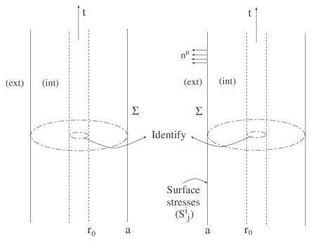
Figure 1: Two copies of static timelike hypersurfaces, $\Sigma$, embedded in asymptotic regions, separating an interior wormhole solution from an exterior vacuum spacetime. Both copies are identified at the wormhole throat, $r_{0}$. The surface stresses reside on $\Sigma$, and members of the normal vector field, $n^{\mu}$, are shown.

The surface mass of the thin shell is given by $M_{\rm shell}=4\pi a^{2}\sigma$ or

$$M_{\rm shell}=a\left(\sqrt{1-\frac{b(a)}{a}}-\sqrt{1-\frac{2M}{a}-\frac{\Lambda}{3}a^{2}}\,\right).$$ (23)

One may interpret $M$ as the total mass of the system, in this case being the total mass of the wormhole in one asymptotic region. Thus, solving equation (23) for $M$, we finally have

$$M=\frac{b(a)}{2}+M_{\rm shell}\left(\sqrt{1-\frac{b(a)}{a}}-\frac{M_{\rm shell}}{2a}\right)-\frac{\Lambda}{6}a^{3}\,.$$ (24)

It is interesting to find some estimates of the surface stresses, for a specific choice of the form function, $b(r)$. Considering dimensionless parameters, equations (21)-(22), for the Schwarzschild-de Sitter solution, take the following form

$$\mu = \xi\left(\sqrt{1-\xi\,\bar{b}(\xi)}-\sqrt{1-\xi-\frac{4\beta}{27\xi^{2}}}\;\right),$$ (25)

$$\Pi = \xi\left(\frac{1-\frac{\xi}{2}-\frac{8\beta}{27\xi^{2}}}{\sqrt{1-\xi-\frac{4\beta}{27\xi^{2}}}}-\zeta\,\sqrt{1-\xi\bar{b}(\xi)}\,\right),$$ (26)

with the following definitions: $\xi=2M/a$, $\beta=9\Lambda M^{2}$, $\bar{b}(\xi)=b(a)/(2M)$, $\mu=8\pi M\sigma$ and $\Pi=16\pi M{\cal P}$. In the analysis that follows we shall assume that $M$ is positive, $M>0$. The surface stresses for the Schwarzschild solution are obtained by setting $\Lambda=0$, i.e., $\beta=0$.

Considering a specific choice of a form function, for instance, $b(r)=r_{0}^{2}/r$, $\mu$ and $\Pi$ are represented in figure 2, for the Schwarzschild solution. We have defined $x=r_{0}/(2M)$, so that for $x>1$ ($r_{0}>2M$), the range of $\xi$ is given by $0<\xi<1/x$. For the $\mu$ plot, we have considered the cases of $x=0.25$, $x=1$ and $x=1.2$, i.e., $r_{0}=M/2$, $r_{0}=2M$ and $r_{0}=2.4M$, respectively. We verify that for $x\leq 1$, one always obtains a non-negative surface energy density, $\mu\geq 0$, whilst for $x>1$ a negative surface energy density is obtained for large values of $\xi$ (for $x=1.2$, the range of $\xi$ is restricted to $0<\xi<0.833$). In relationship to the $\Pi$ plot, we have only considered $x=0.25$ ($r_{0}=M/2$), as the qualitative behaviour for arbitrary $x$ is similar to the one presented. For $\zeta\leq 1$, a surface pressure, $\Pi>0$, is obtained, while for $\zeta>1$, surface tensions are obtained for low values of $\xi$ (high $a$).

Figure 2: The Schwarzschild spacetime, $\Lambda=0$, with the particular choice of $b(r)=r_{0}^{2}/r$. Plots of the surface energy density and surface pressure, are given in terms of dimensionless parameters, i.e., $\mu=8\pi M\sigma$ and $\Pi=16\pi M{\cal P}$, respectively. We have also defined $\xi=2M/a$ and $x=r_{0}/2M$. For $x\leq 1$, a non-negative surface energy density, $\mu\geq 0$, is obtained; for $x>1$, a negative surface energy density is obtained for large values of $\xi$. In the $\Pi$ plot (with $x=0.25$), for $\zeta\leq 1$, we have a surface pressure, $\Pi>0$, while for $\zeta>1$, surface tensions are obtained for low values of $\xi$. See text for details.

For the Schwarzschild-de Sitter case, we have considered $\beta=9\Lambda M^{2}=0.7$. The qualitative behaviour for an arbitrary $\beta$ is similar to the analysis presented in figure 3. For $\beta=0.7$ the black hole and cosmological horizons are given by $r_{b}\simeq 2.33\,M$ and $r_{c}=4.71\,M$, respectively. Thus, only the interval $0.425<\xi<0.858$ is taken into account, as shown in the range of the respective plots. For the $\mu$ plot, we have chosen the values of $x=0.25$, $x=1.165$ and $x=1.3$, i.e., $r_{0}=M/2$, $r_{0}=2.33M=r_{b}$ and $r_{0}=2.6M$, respectively. For $x\leq 1.165$, i.e., $r_{0}\leq r_{b}$, $\mu$ is non-negative; for $x>1.165$, i.e., $r_{0}>r_{b}$, a negative surface energy density is obtained for high values of $\xi$. Recall that for $r_{0}>r_{b}$ the upper limit of $\xi$ is restricted by $\xi<1/x=2M/r_{0}$, so that for the particular case of $\beta=0.7$ and $x=1.3$, we have the range $0.425<\xi<0.769$. The qualitative behaviour of $\Pi$ is transparent from figure 3, where we have considered the cases of $\zeta=0$, $\zeta=1$ and $\zeta=2$, respectively, and $x=0.25$, i.e., $r_{0}=M/2$. The qualitative behaviour of $\Pi$ for arbitrary $x$ is similiar the one presented. For high values of $\xi$ a surface pressure is needed to hold the structure against collapse, and for low $\xi$ a surface tension is needed to hold the wormhole structure against expansion.

One can do an identical analysis for the anti-de Sitter solution, as done in the previous case, however this shall not be attempted here. We shall analyze below the physical properties and characteristics of the surface stresses for generic wormholes, i.e., generic $b(r)$ and $\Phi(r)$.

Figure 3: Plots of $\mu$ and $\Pi$ for the Schwarzschild-de Sitter spacetime, $\Lambda>0$, with the particular choice of $b(r)=r_{0}^{2}/r$ and $\beta=9\Lambda M^{2}=0.7$. The qualitative behaviour for arbitrary $\beta$ is similar to the one presented. The black hole and cosmological horizons are given by $r_{b}\simeq 2.33\,M$ and $r_{c}=4.71\,M$, respectively. For $x\leq 1.165$, i.e., $r_{0}\leq r_{b}$, $\mu$ is non-negative; for $x>1.165$, i.e., $r_{0}>r_{b}$, a negative surface energy density is obtained for high values of $\xi$. In the $\Pi$ graph, we have set $x=0.25$, i.e., $r_{0}=M/2$, with $\zeta=0$, $\zeta=1$ and $\zeta=2$, respectively. For high values of $\xi$ a surface pressure is needed to hold the structure against collapse, and for low $\xi$ a surface tension is needed to hold the wormhole structure against expansion. See text for details.

4.2 The redshift parameter, $\zeta$

To find a physical significance of the parameter $\zeta$, consider the redshift function given by $\Phi(r)=kr^{\alpha}$, with $\alpha,k\in{\bf R}$. Thus, from the definition of $\zeta=1+a\Phi^{\prime}(a)$, the redshift function, in terms of $\zeta$, takes the following form

$$\Phi(r)=\frac{\zeta-1}{\alpha}\,\left(\frac{r}{a}\right)^{\alpha},$$ (27)

with $\alpha\neq 0$, reducing to $\Phi(a)=(\zeta-1)/\alpha$ at the junction surface. Thus, $\zeta$ may also be defined as $\zeta=1+\alpha\Phi(a)$, and one sees that it is related to the gravitational redshift, through the redshift function, at the junction interface. Therefore, one may denote $\zeta$ as the redshift parameter. The proper time on the thin shell is given by $d\tau=e^{\Phi(a)}dt=e^{(\zeta-1)/\alpha}dt$.

The case of $\alpha=0$ corresponds to the constant redshift function, so that $\zeta=1$. If $\alpha<0$, then $\Phi(r)$ is finite throughout spacetime and in the absence of an exterior solution we have $\lim_{r\rightarrow\infty}\Phi(r)\rightarrow 0$. As we are considering a matching of an interior solution with an exterior solution at $a$, then it is also possible to consider the $\alpha>0$ case, imposing that $\Phi(r)$ is finite in the interval $r_{0}\leq r\leq a$.

For the particular case of $\alpha<0$, $\zeta$ is given by $\zeta=1-|\alpha|ka^{\alpha}$. We verify that if $k>0$, then $\zeta<1$ and $\zeta$ takes negative values if $|\alpha|ka^{\alpha}>1$. Thus, the proper time on the thin shell is given by $d\tau=e^{|\zeta-1|/|\alpha|}dt$, and the condition $d\tau>dt$ is verified, i.e., proper time on the thin shell flows faster than the coordinate time, $t$.

If $k<0$, then $\zeta=1+|\alpha||k|a^{\alpha}$ such that $\zeta>1$. $\zeta$ may take large positive values if $\alpha ka^{\alpha}$ is sufficiently large. Thus, $d\tau=e^{-(\zeta-1)/|\alpha|}dt$, with $d\tau<dt$, i.e., proper time on the thin shell flows slower than the coordinate time, $t$.

For the $\alpha>0$ case we are only interested in the range $r_{0}\leq r\leq a$, so that we need to impose that $\Phi(r)$ is finite in the respective domain. We have $\zeta=1+\alpha ka^{\alpha}$, so that if $k>0$ then $\zeta>1$. Therefore $d\tau=e^{(\zeta-1)/\alpha}dt$, implying $d\tau>dt$.

If $k<0$, then from $\zeta=1-\alpha|k|a^{\alpha}$ we have $\zeta<1$. Thus $d\tau=e^{-|\zeta-1|/\alpha}dt$, and therefore $d\tau<dt$, i.e., proper time on the thin shell ticks slower than the coordinate time, $t$.

4.3 Energy conditions on the junction surface

The junction surface may serve to confine the interior wormhole exotic matter to a finite region, which in principle may be made arbitrarily small. Using the notion of the “volume integral quantifier”, equation (6), interior wormhole solutions supported by arbitrarily small quantities of ANEC violating matter were found [6], although the NEC and WEC are always violated for wormhole spacetimes. In the spirit of minimizing the usage of the exotic matter, one may find regions where the surface stress-energy tensor obeys the energy conditions at the junction, $\Sigma$ [2, 28]. Thus, we construct models of spherically symmetric traversable wormholes, where the ANEC violating matter is confined to a region $r_{0}\leq r<a$ (which can be made arbitrarily small by taking the limit $a\to r_{0}$), and the thin shell comprises quasi-normal matter. Here we consider that quasi-normal means matter that satisfies the WEC and NEC (see [6] for similar definitions).

We shall only consider the weak energy condition (WEC) and the null energy condition (NEC). The WEC implies $\sigma\geq 0$ and $\sigma+{\cal P}\geq 0$, and by continuity implies the null energy condition (NEC), $\sigma+{\cal P}\geq 0$.

From equations (21)-(22), we deduce

$$\sigma+{\cal P}=\frac{1}{8\pi a}\left[(2-\zeta)\,\sqrt{1-\frac{b(a)}{a}}-\frac{1-\frac{3M}{a}}{\sqrt{1-\frac{2M}{a}-\frac{\Lambda}{3}a^{2}}}\right].$$ (28)

In the next sections we shall find domains in which the NEC is satisfied, by imposing that the surface energy density is non-negative, $\sigma\geq 0$, i.e., $\sqrt{1-b(a)/a}\geq\sqrt{1-2M/a-\Lambda a^{2}/3}$. A summary of the parameter domain for which the null energy condition is satisfied, for all the cases analyzed, is presented in Table 1.

4.3.1 Schwarzschild solution.

Consider the Schwarzschild solution, $\Lambda=0$. We are interested in finding the regions in which the WEC and the NEC at the junction are satisfied, by imposing a non-negative surface energy density, $\sigma\geq 0$, i.e., $\sqrt{1-b(a)/a}\geq\sqrt{1-2M/a}$. For the particular case of $\zeta\leq 1$, from equation (28) we verify that $\sigma+{\cal P}\geq 0$ is readily satisfied for $\forall\,a$.

For $1<\zeta<2$, the NEC is verified in the following region

$$2M<a\leq 2M\,\left(\frac{\zeta-\frac{1}{2}}{\zeta-1}\right).$$ (29)

For convenience, by defining a new parameter $\xi=2M/a$, equation (29) takes the form

$$\frac{\zeta-1}{\zeta-\frac{1}{2}}\leq\xi<1\,.$$ (30)

For $\zeta=2$, the NEC is satisfied for $\xi\geq 2/3$, i.e., $a\leq 3M$. For $\zeta>2$, we need to impose the NEC in the region of equation (30); with $\sigma+{\cal P}<0$ for $\xi<(\zeta-1)/(\zeta-1/2)$. See Table 1 for a summary of the cases analyzed.

4.3.2 Schwarzschild-de Sitter solution.

For the Schwarzschild-de Sitter spacetime, $\Lambda>0$, we shall once again impose a non-negative surface energy density, $\sigma\geq 0$. Consider the definitions $\beta=9\Lambda M^{2}$ and $\xi=2M/a$.

For $\zeta<2$ the condition $\sigma+{\cal P}\geq 0$ is readily met for $\beta\leq\beta_{0}$, with $\beta_{0}$ given by

$$\beta_{0}=\frac{27}{4}\,\frac{\xi^{2}}{(2-\zeta)}\,\left[(1-\zeta)+\left(\zeta-\frac{1}{2}\right)\xi\right].$$ (31)

Choosing a particular example, for instance $\zeta=-0.5$, consider figure 4. The region of interest is shown below the solid line, which is given by $\beta_{r}=27\xi^{2}(1-\xi)/4$. The case of $\zeta=-0.5$ is depicted as a dashed curve, and the NEC is obeyed to the right of the latter.

For $\zeta=2$, then the NEC is verified for $\forall\,\beta$ and $\xi\geq 2/3$, i.e., $r_{b}<a\leq 3M$, with $r_{b}$ given by equation (9). This analysis is depicted in figure 4, with the NEC being satisfied to the right of the dashed curve, represented by $\zeta=2$.

For the case of $\zeta>2$, the condition $\sigma+{\cal P}\geq 0$ needs to be imposed in the region $\beta_{0}\leq\beta\leq\beta_{r}$; and $\sigma+{\cal P}<0$ for $\beta<\beta_{0}$. The specific case of $\zeta=5$ is depicted as a dashed curve in figure 4. The NEC needs to be imposed to the right of the respective curve. See Table 1 for a summary of the cases analyzed.

Figure 4: Analysis of the null energy condition for the Schwarzschild-de Sitter spacetime. We have considered the definitions $\beta=9\Lambda M^{2}$ and $\xi=2M/a$. Only the region below the solid line is of interest. We have considered specific examples, and the NEC is obeyed to the right of each respective dashed curves, $\zeta=-0.5$, $\zeta=2$ and $\zeta=5$. See text for details.

4.3.3 Schwarzschild-anti de Sitter solution.

Considering the Schwarzschild-anti de Sitter spacetime, $\Lambda<0$, once again a non-negative surface energy density, $\sigma\geq 0$, is imposed. Consider the definitions $\gamma=9|\Lambda|M^{2}$ and $\xi=2M/a$.

For $\zeta\leq 1$ the condition $\sigma+{\cal P}\geq 0$ is readily met for $\forall\,\gamma$ and $\forall\,\xi$. For $1<\zeta<2$, the NEC is satisfied in the region $\gamma\geq\gamma_{0}$, with $\gamma_{0}$ given by

$$\gamma_{0}=\frac{27}{4}\,\frac{\xi^{2}}{(2-\zeta)}\,\left[(\zeta-1)-\left(\zeta-\frac{1}{2}\right)\xi\right].$$ (32)

The particular case of $\zeta=1.8$ is depicted in figure 5. The region of interest is delimited by the $\xi$-axis and the area to the left of the solid curve, which is given by $\gamma_{r}=27\xi^{2}(\xi-1)/4$. Thus, the NEC is obeyed above the dashed curve represented by the value $\zeta=1.8$.

For $\zeta=2$, then $\sigma+{\cal P}\geq 0$ is verified for $\forall\gamma$ and $\xi\geq 3/2$, i.e., $r_{b}<a\leq 3M$, with $r_{b}$ given by equation (11). Therefore, the NEC is obeyed to the right of the dashed curve represented by $\zeta=2$, and to the left of the solid line, $\gamma_{r}$.

For the case of $\zeta>2$, the condition $\sigma+{\cal P}\geq 0$ needs to be imposed in the region $\gamma_{r}\leq\gamma\leq\gamma_{0}$. The specific case of $\zeta=3$ is depicted in figure 5 as a dashed curve. Thus, the NEC needs to be imposed in the region to the right of the respective dashed curve and to the left of the solid line, $\gamma_{r}$. See Table 1 for a summary of the cases analyzed.

Figure 5: Analysis of the null energy condition for the Schwarzschild-anti de Sitter spacetime. We have considered the definitions $\gamma=9|\Lambda|M^{2}$ and $\xi=2M/a$. The only area of interest is depicted to the left of the solid curve, given by $\gamma_{r}=27\xi^{2}(\xi-1)/4$. For the specific case of $\zeta=1.8$, the NEC is obeyed above the respective curve. For the cases of $\zeta=2$ and $\zeta=3$, the NEC is verified to the right of the respective dashed curves, and to the left of the solid line. See text for details.

$\Lambda=0$	$\zeta\leq 1$	$\forall\,\xi$
	$\zeta>1$	$(\zeta-1)/(\zeta-1/2)\leq\xi<1$
	$\zeta<2$	$\beta\leq\beta_{0}$
$\Lambda>0$	$\zeta=2$	$\forall\,\beta$  and  $\xi\geq 2/3$
	$\zeta>2$	$\beta_{0}\leq\beta\leq\beta_{r}$
	$\zeta\leq 1$	$\forall\,\gamma$  and  $\forall\,\xi$
$\Lambda<0$	$1<\zeta<2$	$\gamma\geq\gamma_{0}$
	$\zeta=2$	$\forall\,\gamma$  and  $\xi\geq 3/2$
	$\zeta>2$	$\gamma_{r}\leq\gamma\leq\gamma_{0}$

Table 1: Parameter domain for which the null energy condition is satisfied, i.e., $\sigma+{\cal P}\geq 0$, by imposing a positive surface energy density, i.e., $\sigma\geq 0$. We have defined the parameters $\xi=2M/a$, $\beta=9\Lambda M^{2}$ and $\gamma=9|\Lambda|M^{2}$; $\beta_{0}$ and $\gamma_{0}$ are given by equation (31) and equation (32), respectively. See text for details.

4.4 Physical properties and characteristics of the surface stresses

In this section we shall consider some interesting physical properties and characteristics of the surface stresses for generic wormholes by eliminating the form function $b(r)$, and writing ${\cal P}$ as a function of $\sigma$. Thus, taking into account equations (21)-(22), one may express ${\cal P}$ as a function of $\sigma$ by the following relationship

$${\cal P}=\frac{1}{8\pi a}\,\left[\frac{(1-\zeta)+(\zeta-\frac{1}{2})\,\frac{2M}{a}-(2-\zeta)\frac{\Lambda}{3}a^{2}}{\sqrt{1-\frac{2M}{a}-\frac{\Lambda}{3}a^{2}}}-4\pi a\zeta\sigma\right].$$ (33)

We shall analyze equation (33), namely, find domains in which ${\cal P}$ assumes the nature of a tangential surface pressure, ${\cal P}>0$, or a tangential surface tension, ${\cal P}<0$, for the Schwarzschild case, $\Lambda=0$, the Schwarzschild-de Sitter spacetime, $\Lambda>0$, and for the Schwarzschild-anti de Sitter solution, $\Lambda<0$. In the analysis that follows we shall consider that $M$ is positive, $M>0$.

4.4.1 Schwarzschild spacetime.

For the Schwarzschild spacetime, $\Lambda=0$, equation (33) reduces to

$${\cal P}=\frac{1}{8\pi a}\,\left[\frac{(1-\zeta)+(\zeta-\frac{1}{2})\,\frac{2M}{a}}{\sqrt{1-\frac{2M}{a}}}-4\pi a\zeta\sigma\right]\,.$$ (34)

To find domains in which ${\cal P}$ is a tangential surface pressure, ${\cal P}>0$, or a tangential surface tension, ${\cal P}<0$, it is convenient to express equation (34) in the following compact form

$${\cal P}=\frac{1}{16\pi M}\,\frac{\Gamma(\xi,\zeta,\mu)}{\sqrt{1-\xi}}\,,$$ (35)

with the dimensionless parameters given by $\xi=2M/a$ and $\mu=8\pi M\sigma$. $\Gamma(\xi,\zeta,\mu)$ is defined as

$$\Gamma(\xi,\zeta,\mu)=(1-\zeta)\,\xi+\left(\zeta-\frac{1}{2}\right)\xi^{2}-\mu\zeta\sqrt{1-\xi}\;.$$ (36)

One may now fix one or several of the parameters and analyze the sign of $\Gamma(\xi,\zeta,\mu)$, and consequently the sign of ${\cal P}$.

a. Fixed $\zeta$, varying $\xi$ and $\mu$.

In this section we shall analyze the specific case of a fixed value of $a\Phi^{\prime}(a)$ and vary the values of the junction radius, $a$, and of the surface energy density, $\sigma$, i.e., consider a fixed value of the redshift parameter $\zeta$, varying the parameters $(\xi,\mu)$. To analyze the sign of ${\cal P}$, it is useful to consider a null tangential surface pressure, ${\cal P}=0$, i.e., $\Gamma(\xi,\zeta,\mu)=0$. Thus, from equation (36) we have

$$\mu_{0}=\frac{(1-\zeta)\xi+(\zeta-1/2)\xi^{2}}{\zeta\sqrt{1-\xi}}\,,$$ (37)

with $\zeta\neq 0$. It is necessary to separate the cases of $\zeta=0$, $\zeta>0$ and $\zeta<0$, respectively.

Firstly, for the case of $\zeta=0$, equation (36) reduces to $\Gamma(\xi,\zeta=0,\mu)=\xi-\xi^{2}/2$, which is always positive, as $0<\xi<1$, implying a tangential surface pressure, ${\cal P}>0$.

Secondly, for $\zeta>0$, a tangential surface pressure, ${\cal P}>0$, is provided for $\mu<\mu_{0}$, and a tangential surface tension, ${\cal P}<0$, for $\mu>\mu_{0}$. Note that a surface boundary, with ${\cal P}=0$ and $\sigma=0$, is given by $\xi=(\zeta-1)/(\zeta-1/2)$, for $\zeta>1$. For $0<\zeta\leq 1$, we have a positive surface energy density, $\mu_{0}>0$, thus satisfying the energy conditions, which is consistent with the results of the previous section. The qualitative behavior for $\zeta>0$ can be represented by the specific case of $\zeta=1$, corresponding to a constant redshift function, depicted in figure 6. For non-positive values of $\mu$ and $\forall\,\xi$ a surface pressure, ${\cal P}>0$, is required to hold the thin shell structure against collapse. Close to the black hole event horizon, $a\rightarrow 2M$, i.e. $\xi\rightarrow 1$, a surface pressure is also needed to hold the structure against collapse. For high values of $\mu$ and low values of $\xi$, a surface tangential tension, ${\cal P}<0$, is needed to hold the structure against expansion. In particular, for the constant redshift function, $\Phi^{\prime}(r)=0$, and a null surface energy density, $\sigma=0$, i.e., $\zeta=1$ and $\mu=0$, respectively, equation (36) reduces to $\Gamma(\xi)=\xi^{2}/2$, from which we readily conclude that ${\cal P}$ is non-negative everywhere, tending to zero at infinity, i.e., $\xi\rightarrow 0$. This is a particular case analyzed in [24].

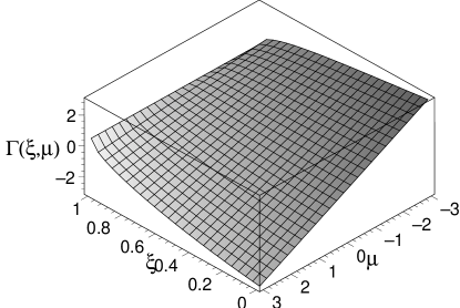
Figure 6: The surface represents the sign of ${\cal P}$ for the Schwarzschild spacetime with a constant redshift function, $\Phi^{\prime}(r)=0$, i.e., $\zeta=1$. For non-positive values of $\mu$ and $\forall\,\xi$, we have a surface tangential pressure, ${\cal P}>0$. For extremely high values of $\xi$ (close to the black hole event horizon) and $\forall\,\mu$, a surface pressure is also required to hold the structure against collapse. For high values of $\mu$ and low values of $\xi$, we have a tangential surface tension, ${\cal P}<0$, to hold the structure against expansion. See text for details.

$\xi=0$	$\Gamma(\xi=0,\zeta,\mu)>0$  for  $\forall\,\mu$
$\xi>0$	$\Gamma(\xi,\zeta,\mu)>0$  for  $\mu<\mu_{0}$
	$\Gamma(\xi,\zeta,\mu)<0$  for  $\mu>\mu_{0}$
$\xi<0$	$\Gamma(\xi,\zeta,\mu)>0$  for  $\mu>\mu_{0}$
	$\Gamma(\xi,\zeta,\mu)<0$  for  $\mu<\mu_{0}$

Table 2: The parameter domain of the sign of ${\cal P}$ for the Schwarzschild solution. ${\cal P}$ is a tangential surface pressure if $\Gamma(\xi,\zeta,\mu)>0$, and a surface tension if $\Gamma(\xi,\zeta,\mu)<0$. $\Gamma(\xi,\zeta,\mu)$ and $\mu_{0}$ are given by equation (36) and equation (37), respectively.. See text for details.

Finally, for the $\zeta<0$ case, we verify that a surface pressure, ${\cal P}>0$, is obtained for $\mu>\mu_{0}$, and a tangential surface tension, ${\cal P}<0$, for $\mu<\mu_{0}$, contrary to the $\zeta>0$ analysis. The specific case of $\zeta=-1$, depicted in figure 7, can be considered representative for the qualitative behavior of $\zeta<0$. For non-negative values of $\mu$ and for $\forall\,\xi$, a surface pressure, ${\cal P}>0$, is required. Close to the black hole event horizon, i.e., for high values of $\xi$, and for $\forall\,\mu$, a surface pressure is also required to hold the structure against collapse. For low negative values of $\mu$ and for low values of $\xi$, a surface tension is needed, which is somewhat intuitive as a negative surface energy density is gravitationally repulsive, requiring a surface tension to hold the structure against expansion. See Table 2 for a summary of the results obtained.

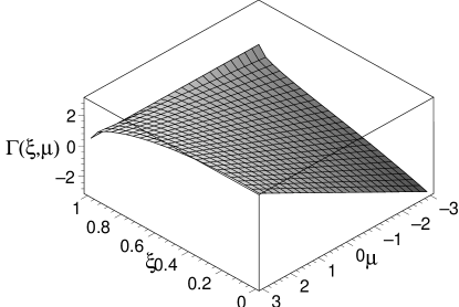
Figure 7: The surface is given by equation (36) for the Schwarzschild spacetime with $\zeta=-1$. For non-negative values of $\mu$ and $\forall\,\xi$, we have a surface tangential pressure, ${\cal P}>0$. For high values of $\xi$, i.e., close to the black hole event horizon, and for $\forall\,\mu$, a surface pressure is also required to hold the structure against collapse. For negative values of $\mu$ and low $\xi$, a tangential surface tension, ${\cal P}<0$, is required to hold the structure against expansion. See text for details.

b. Fixed $\mu$, varying $\xi$, and $\zeta$.

In this section we shall consider an alternative analysis. We shall study the case of a fixed value for the surface energy density, $\sigma$, and vary the values of the junction surface, $a$, and of $a\Phi^{\prime}(a)$, i.e., we fix the parameter $\mu$, varying $\xi$ and $\zeta$. Equation (36) may be rewritten in the form

$$\Gamma(\xi,\zeta,\mu)=\xi\,\left(1-\frac{\xi}{2}\right)-\sqrt{1-\xi}\left(\xi\sqrt{1-\xi}-\mu\right)\zeta\,.$$ (38)

Once again to analyze the sign of ${\cal P}$, we consider a null tangential surface pressure, i.e., $\Gamma(\xi,\zeta,\mu)=0$. Thus, from equation (38) one finds the following relationship

$$\zeta_{0}=\frac{\xi(1-\xi/2)}{\sqrt{1-\xi}\left(\xi\,\sqrt{1-\xi}-\mu\right)}\,,$$ (39)

with $\mu\neq\xi\sqrt{1-\xi}$.

For the specific case of $\mu=\xi\sqrt{1-\xi}$, equation (38) reduces to $\Gamma(\xi,\zeta,\mu)=\xi(1-\xi/2)$, which is always positive, implying a surface pressure. For this case $\mu$ attains a maximum at $\mu_{\rm max}=2\sqrt{3}/9$ for $\xi=2/3$, i.e., $a=3M$. Therefore, for fixed values of $\mu$ in the interval $0<\mu<2\sqrt{3}/9$, one has three regions to analyze the sign of ${\cal P}$. Consider, for simplicity, the specific case of $\mu=1.7\sqrt{3}/9$, represented in figure 8. The regions corresponding to the surface tensions are shown. As $\mu\rightarrow 0$ the intermediate region expands outwards to the points $\xi\rightarrow 0$ and $\xi\rightarrow 1$, respectively; as $\mu\rightarrow 2\sqrt{3}/9$, the intermediate region contracts to the point $\xi\rightarrow 2/3$.

Figure 8: The curves are given by equation (39) for the range $0<\mu<2\sqrt{3}/9$. We consider a particular example, i.e., $\mu=1.7\sqrt{3}/9$. The area above the curve in the intermediate region, and below the curves in the two outer regions, correspond to surface tensions. The intermediate region expands outwards to the points $\xi\rightarrow 0$ and $\xi\rightarrow 1$, respectively, as $\mu\rightarrow 0$, and contracts to the point $\xi\rightarrow 2/3$, as $\mu\rightarrow 2\sqrt{3}/9$. See text for details.

For $\mu<\xi\sqrt{1-\xi}$, we have $\Gamma(\xi,\zeta,\mu)>0$, implying a surface pressure, ${\cal P}>0$, for $\zeta<\zeta_{0}$; and $\Gamma(\xi,\zeta,\mu)<0$, providing a surface tension, ${\cal P}<0$, for $\zeta>\zeta_{0}$. The analysis for non-positive values of the surface energy density, $\sigma\leq 0$, is fairly straightforward. The qualitative behavior for $\mu\leq 0$ is similar to that of the cases presented in figure 9, namely, that of $\mu=0$ and $\mu=-1$, respectively. Below the respective curves, we have a surface pressure, ${\cal P}>0$, and above the respective curves, we have a surface tension, ${\cal P}<0$.

Finally, for $\mu>\xi\sqrt{1-\xi}$, one has a surface pressure, ${\cal P}>0$, for $\zeta>\zeta_{0}$; and a surface tension, ${\cal P}<0$, for $\zeta<\zeta_{0}$. For values of $\mu>2\sqrt{3}/9$, the qualitative behavior is similar to the cases of $\mu=0.5$ and $\mu=1$, which are represented in figure 9. Above the respective curves, we have a surface pressure, ${\cal P}>0$, and below the curves, a surface tension, ${\cal P}<0$.

Figure 9: The curves are given by equation (39). For the cases of $\mu=0$ and $\mu=-1$ represented, below the respective curves we have a surface pressure, ${\cal P}>0$, and above the curves, a surface tension, ${\cal P}<0$. For the cases of $\mu=0.5$ and $\mu=1$, we have the inverse behavior, i.e., below the respective curves we have a surface tension, ${\cal P}<0$, and above the curves a surface pressure, ${\cal P}>0$. See text for details.

c. Fixed $\xi$, varying $\zeta$ and $\mu$.

For an alternative analysis consider a fixed value for the junction radius, $a$, varying $a\Phi^{\prime}(a)$ and the surface energy density, $\sigma$, i.e., we fix $\xi$ and vary the parameters $\zeta$ and $\mu$. Equation (36) with $\xi=0$, reduces to $\Gamma(\xi=0,\zeta,\mu)=-\mu\,\zeta$. Qualitatively, we verify that for either positive values for both $\zeta$ and $\mu$, or for negative values for both $\zeta$ and $\mu$, we have $\Gamma(\xi=0,\zeta,\mu)<0$, implying a surface tension. If $\zeta$ is negative and $\mu$ positive, or vice-versa, we verify that $\Gamma(\xi=0,\zeta,\mu)>0$, implying a tangential surface pressure. Now, as $\xi$ increases from $0$ to $1$, $\Gamma(\zeta,\mu)$ attains the value of a constant surface $\Gamma(\xi=1,\zeta,\mu)\rightarrow 1/2$, as $\xi\rightarrow 1$, i.e., $a\rightarrow 2M$, is reached.

4.4.2 Schwarzschild-de Sitter spacetime.

For the Schwarzschild-de Sitter spacetime with $\Lambda>0$, to analyze the sign of ${\cal P}$, it is convenient to express equation (33) in the following compact form

$${\cal P}=\frac{1}{16\pi M}\,\frac{\Gamma(\xi,\zeta,\mu,\beta)}{\sqrt{1-\xi-\frac{4\beta}{27\xi^{2}}}}\,,$$ (40)

with $\xi=2M/a$, $\mu=8\pi M\sigma$ and $\beta=9\Lambda M^{2}$. $\Gamma(\xi,\zeta,\mu,\beta)$ is defined as

$$\Gamma(\xi,\zeta,\mu,\beta) = (1-\zeta)\,\xi+\left(\zeta-\frac{1}{2}\right)\xi^{2}-\frac{4\beta}{27\xi}\,(2-\zeta)$$ (41)

$$-\mu\zeta\sqrt{1-\xi-\frac{4\beta}{27\xi^{2}}}\;.$$

To analyze the sign of $\Gamma(\xi,\zeta,\mu,\beta)$, and consequently the sign of ${\cal P}$, one may fix several of the parameters.

a. Null surface energy density.

Consider a null surface energy density, $\sigma=0$, i.e., $\mu=0$. Thus, equation (41) reduces to

$$\Gamma(\xi,\zeta,\beta)=(1-\zeta)\,\xi+\left(\zeta-\frac{1}{2}\right)\,\xi^{2}-(2-\zeta)\,\frac{4\beta}{27\xi}\,.$$ (42)

To analyze the sign of ${\cal P}$, we shall consider a null tangential surface pressure, i.e., $\Gamma(\xi,\zeta,\beta)=0$, so that from equation (42) we have the following relationship

$$\beta_{0}=\frac{27}{4}\frac{\xi^{2}}{(2-\zeta)}\left[(1-\zeta)+\left(\zeta-\frac{1}{2}\right)\,\xi\right]\,,$$ (43)

with $\zeta\neq 2$, which is identical to equation (31).

For the particular case of $\zeta=2$, from equation (42), we have $\Gamma(\xi,\zeta=2,\beta)=\xi(3\xi/2-1)$. A surface boundary, $\Gamma(\xi,\zeta=2,\beta)=0$, is presented at $\xi=2/3$, i.e., $a=3M$. A surface pressure, $\Gamma(\xi,\zeta=2,\beta)>0$, is given for $\xi>2/3$, i.e., $r_{b}<a<3M$, and a surface tension, $\Gamma(\xi,\zeta=2,\beta)<0$, for $\xi<2/3$, i.e., $3M<a<r_{c}$.

For $\zeta<2$, from equation (42), a surface pressure, $\Gamma(\xi,\zeta,\beta)>0$, is met for $\beta<\beta_{0}$, and a surface tension, $\Gamma(\xi,\zeta,\beta)<0$, for $\beta>\beta_{0}$. The specific case of a constant redshift function, i.e., $\zeta=1$, is analyzed in [24] (For this case, equation (43) is reduced to $\beta_{0}=27\xi^{3}/8$, or $M=\Lambda a^{3}/3$). For the qualitative behavior, the reader is referred to the particular case of $\zeta=-0.5$ provided in figure 4. To the right of the curve a surface pressure, ${\cal P}>0$, is given and to the left of the respective curve a surface tension, ${\cal P}<0$. One verifies that as $\zeta\rightarrow-\infty$, the curve superimposes with the solid line, $\beta_{r}$, and one only has a surface pressure for the entire region of interest.

For $\zeta>2$, from equation (42), a surface pressure, $\Gamma(\xi,\zeta,\beta)>0$, is given for $\beta_{0}<\beta<\beta_{r}$, and a surface tension, $\Gamma(\xi,\zeta,\beta)<0$, for $\beta<\beta_{0}$. Once again the reader is referred to figure 4 for a qualitative analysis of the behavior for the particular case of $\zeta=5$. A surface pressure is given to the right of the curve and a surface tension to the left. For $\zeta\rightarrow+\infty$, the curve superimposes with the solid line, $\beta_{r}$, and a surface tension is given for the entire region of interest.

Note that for the analysis considered in this section, namely, for a null surface energy density, the WEC, and consequently the NEC, are satisfied only if ${\cal P}\geq 0$. The results obtained are consistent with those of the section regarding the energy conditions at the junction surface, for the Schwarzschild-de Sitter spacetime, considered above. See Table 3 for a summary of the results obtained.

$\zeta<2$	$\Gamma(\xi,\zeta,\beta)>0$,  $\beta<\beta_{0}$
	$\Gamma(\xi,\zeta,\beta)<0$,  $\beta>\beta_{0}$
	$\Gamma(\xi,\zeta=2,\beta)=0$,  $\forall\,\beta$  and  $\xi=2/3$
$\zeta=2$	$\Gamma(\xi,\zeta=2,\beta)>0$,  $\forall\,\beta$  and  $\xi>2/3$
	$\Gamma(\xi,\zeta=2,\beta)<0$,  $\forall\,\beta$  and  $\xi<2/3$
$\zeta>2$	$\Gamma(\xi,\zeta,\beta)>0$,  $\beta_{0}<\beta<\beta_{r}$
	$\Gamma(\xi,\zeta,\beta)<0$,  $\beta<\beta_{0}$

Table 3: The parameter domain of the sign of ${\cal P}$, for the Schwarzschild-de Sitter solution, $\Lambda>0$. Considering the particular case of a null surface energy density, i.e., $\mu=0$, ${\cal P}$ is a tangential surface pressure if $\Gamma(\xi,\zeta,\beta)>0$, and a surface tension if $\Gamma(\xi,\zeta,\beta)<0$. $\Gamma(\xi,\zeta,\beta)$ and $\beta_{0}$ are given by equation (42) and equation (43), respectively. See text for details.

b. Constant redshift function.

We shall next consider a constant redshift function, $\Phi^{\prime}(r)=0$, i.e., $\zeta=1$. Thus equation (41) is reduced to

$$\Gamma(\xi,\mu,\beta)=\frac{\xi^{2}}{2}-\frac{4\beta}{27\xi}-\mu\,\sqrt{1-\xi-\frac{4\beta}{27\xi^{2}}}\,.$$ (44)

Considering a null tangential surface pressure, $\Gamma(\xi,\mu,\beta)=0$, equation (44) takes the following form

$$\mu_{0}=\frac{\frac{\xi^{2}}{2}-\frac{4\beta}{27\xi}}{\sqrt{1-\xi-\frac{4\beta}{27\xi^{2}}}}\,.$$ (45)

We verify that a surface pressure, ${\cal P}>0$, is given for $\mu<\mu_{0}$, and a surface tension, ${\cal P}<0$, for $\mu>\mu_{0}$. A surface boundary, $\mu_{0}=0$, is verified for $\beta_{0}=27\xi^{3}/8$.

4.4.3 Schwarzschild-anti de Sitter spacetime.

For the Schwarzschild-anti de Sitter spacetime, $\Lambda<0$, to analyze the sign of ${\cal P}$, equation (33) is expressed as

$${\cal P}=\frac{1}{16\pi M}\,\frac{\Gamma(\xi,\zeta,\mu,\gamma)}{\sqrt{1-\xi+\frac{4\gamma}{27\xi^{2}}}}\,,$$ (46)

with the parameters given by $\xi=2M/a$, $\mu=8\pi M\sigma$ and $\gamma=9|\Lambda|M^{2}$, respectively. $\Gamma(\xi,\zeta,\mu,\gamma)$ is defined as

$$\Gamma(\xi,\zeta,\mu,\gamma) = (1-\zeta)\,\xi+\left(\zeta-\frac{1}{2}\right)\xi^{2}+\frac{4\gamma}{27\xi}\,(2-\zeta)$$ (47)

$$-\mu\zeta\sqrt{1-\xi+\frac{4\gamma}{27\xi^{2}}}\;.$$

As in the Schwarzschild-de Sitter solution we shall analyze the cases of a null surface energy density, $\sigma=0$, and a constant redshift function, $\Phi^{\prime}(r)=0$, i.e., $\mu=0$ and $\zeta=1$, respectively.

a. Null surface energy density.

For a null surface energy density, $\sigma=0$, i.e., $\mu=0$, equation (47) reduces to

$$\Gamma(\xi,\zeta,\gamma)=(1-\zeta)\,\xi+\left(\zeta-\frac{1}{2}\right)\,\xi^{2}+(2-\zeta)\,\frac{4\gamma}{27\xi}\,,$$ (48)

To analyze the sign of ${\cal P}$, once again we shall consider a null tangential surface pressure, i.e., $\Gamma(\xi,\zeta,\gamma)=0$, so that from equation (48) we have

$$\gamma_{0}=\frac{27}{4}\frac{\xi^{2}}{(2-\zeta)}\left[(\zeta-1)-\left(\zeta-\frac{1}{2}\right)\,\xi\right]\,,$$ (49)

with $\zeta\neq 2$, which is identical to equation (32).

For the particular case of $\zeta=2$, from equation (48), we have $\Gamma(\xi,\zeta=2,\gamma)=\xi(3\xi/2-1)$, which is null at $\xi=2/3$, i.e., $a=3M$. A surface pressure, $\Gamma(\xi,\zeta=2,\gamma)>0$, is given for $\xi>2/3$, i.e., $r_{b}<a<3M$, and a surface tension, $\Gamma(\xi,\zeta=2,\gamma)<0$, for $\xi<2/3$, i.e., $a>3M$. The reader is referred to the particular case of $\zeta=2$, depicted in figure 5. A surface pressure is given to the right of the respective dashed curve, and a surface tension to the left.

For $\zeta\leq 1$, a surface pressure, $\Gamma(\xi,\zeta,\gamma)>0$, is given for $\forall\;\gamma$ and $\forall\;\xi$. For $1<\zeta<2$, a surface pressure, $\Gamma(\xi,\zeta,\gamma)>0$, is given for $\gamma>\gamma_{0}>0$; and a surface tension, $\Gamma(\xi,\zeta,\gamma)<0$, is provided for $0<\gamma<\gamma_{0}$. The particular case of $\zeta=1.8$ is depicted in figure 5, in which a surface pressure is presented above the respective dashed curve, and a surface tension is presented in the region delimited by the curve and the $\xi$-axis.

For $\zeta>2$, a surface pressure, $\Gamma(\xi,\zeta,\gamma)>0$, is met for $\gamma_{r}<\gamma<\gamma_{0}$, and a surface tension, $\Gamma(\xi,\zeta,\gamma)<0$, for $\gamma>\gamma_{0}$. The specific case for $\zeta=3$ is depicted in figure 5. A surface pressure is presented to the right of the respective curve, and a surface tension to the left.

Once again, the analysis considered in this section is consistent with the results obtained in the section regarding the energy conditions at the junction surface, for the Schwarzschild-anti de Sitter spacetime, considered above. This is due to the fact that for the specific case of a null surface energy density, the regions in which the WEC and NEC are satisfied coincide with the range of ${\cal P}\geq 0$. See Table 4 for a summary of the results obtained.

$\zeta\leq 1$	$\Gamma(\xi,\zeta,\gamma)>0$,  $\forall\,\gamma$  and  $\forall\,\xi$
$1<\zeta<2$	$\Gamma(\xi,\zeta,\gamma)>0$,  $\gamma>\gamma_{0}>0$
	$\Gamma(\xi,\zeta,\gamma)<0$,  $0<\gamma<\gamma_{0}$
	$\Gamma(\xi,\zeta=2,\gamma)=0$,  $\forall\,\gamma$  and  $\xi=2/3$
$\zeta=2$	$\Gamma(\xi,\zeta=2,\gamma)>0$,  $\forall\,\gamma$  and  $\xi>2/3$
	$\Gamma(\xi,\zeta=2,\gamma)<0$,  $\forall\,\gamma$  and  $\xi<2/3$
$\zeta>2$	$\Gamma(\xi,\zeta,\gamma)>0$,  $\gamma_{r}<\gamma<\gamma_{0}$
	$\Gamma(\xi,\zeta,\gamma)<0$,  $\gamma>\gamma_{0}$

Table 4: The parameter domain for the sign of ${\cal P}$, considering the Schwarzschild-anti de Sitter solution, $\Lambda<0$. Considering the particular case of a null surface energy density, i.e., $\mu=0$, ${\cal P}$ is a tangential surface pressure if $\Gamma(\xi,\zeta,\gamma)>0$, and a surface tension if $\Gamma(\xi,\zeta,\gamma)<0$. $\Gamma(\xi,\zeta,\gamma)$ and $\gamma_{0}$ are given by equation (48) and equation (49), respectively. See text for details.

b. Constant redshift function.

For the case of a constant redshift function, $\Phi^{\prime}(r)=0$, i.e., $\zeta=1$, equation (47) is reduced to

$$\Gamma(\xi,\mu,\gamma)=\frac{\xi^{2}}{2}+\frac{4\gamma}{27\xi}-\mu\,\sqrt{1-\xi+\frac{4\gamma}{27\xi^{2}}}\,.$$ (50)

To analyze the sign of ${\cal P}$, consider $\Gamma(\xi,\mu,\gamma)=0$, so that equation (50) takes the following form

$$\mu_{0}=\frac{\frac{\xi^{2}}{2}+\frac{4\gamma}{27\xi}}{\sqrt{1-\xi+\frac{4\gamma}{27\xi^{2}}}}\,,$$ (51)

which is always positive. A surface pressure, ${\cal P}>0$, is given for $0<\mu<\mu_{0}$, and a surface tension, ${\cal P}<0$, for $\mu>\mu_{0}$.

4.5 Pressure balance equation

One may obtain an equation governing the behavior of the radial pressure in terms of the surface stresses at the junction boundary from the following identity [2, 29]

$$\left[\,T^{\rm total}_{\hat{\mu}\hat{\nu}}\,n^{\hat{\mu}}n^{\hat{\nu}}\right]=\frac{1}{2}(K^{i\;+}_{\;\,j}+K^{i\;-}_{\;\,j})\,S^{j}_{\;\,i}\,,$$ (52)

where $T^{\rm total}_{\hat{\mu}\hat{\nu}}=T_{\hat{\mu}\hat{\nu}}-g_{\hat{\mu}\hat{\nu}}\,\Lambda/8\pi$ is the total stress-energy tensor, and the square brackets denotes the discontinuity across the thin shell, i.e., $[X]=X^{+}|_{\Sigma}-X^{-}|_{\Sigma}$. Taking into account the values of the extrinsic curvatures, equations (17)-(20), and noting that the tension acting on the shell is by definition the normal component of the stress-energy tensor, $-\tau=T_{\hat{\mu}\hat{\nu}}\,n^{\hat{\mu}}n^{\hat{\nu}}$, we finally have the following pressure balance equation

$$\left(-\tau^{+}(a)-\frac{\Lambda^{+}}{8\pi}\right)-\left(-\tau^{-}(a)-\frac{\Lambda^{-}}{8\pi}\right)=\frac{1}{a}\,\left(\sqrt{1-\frac{2M}{a}-\frac{\Lambda}{3}a^{2}}+\sqrt{1-\frac{b(a)}{a}}\;\right)\,{\cal P}$$

$$-\left(\frac{\frac{M}{a^{2}}-\frac{\Lambda}{3}a}{\sqrt{1-\frac{2M}{a}-\frac{\Lambda}{3}a^{2}}}+\Phi^{\prime}(a)\,\sqrt{1-\frac{b(a)}{a}}\right)\frac{\sigma}{2},$$ (53)

where the $\pm$ superscripts correspond to the exterior and interior spacetimes, respectively. Equation (4.5) relates the difference of the radial tension across the shell in terms of a combination of the surface stresses, $\sigma$ and ${\cal P}$, given by equations (21)-(22), respectively, and the geometrical quantities.

Note that for the exterior vacuum solution we have $\tau^{+}=0$. For the particular case of a null surface energy density, $\sigma=0$, and considering that the interior and exterior cosmological constants are equal, $\Lambda^{-}=\Lambda^{+}$, equation (4.5) reduces to

$$\tau^{-}(a)=\frac{2}{a}\,\sqrt{1-\frac{2M}{a}-\frac{\Lambda}{3}a^{2}}\;\,{\cal P}\,.$$ (54)

For a radial tension, $\tau^{-}(a)>0$, acting on the shell from the interior, a tangential surface pressure, ${\cal P}>0$, is needed to hold the thin shell form collapsing. For a radial interior pressure, $\tau^{-}(a)<0$, then a tangential surface tension, ${\cal P}<0$, is needed to hold the structure form expansion.

5 Conclusion

We have constructed wormhole solutions by matching an interior solution to a vacuum exterior spacetime, with a generic cosmological constant, at a junction surface. In the spirit of minimizing the usage of exotic matter, regions satisfying the weak and null energy conditions at the junction surface were determined. Thus, models of spherically symmetric traversable wormholes were constructed where the null energy condition violating matter is confined to the region $r_{0}\leq r<a$, while quasi-normal matter resides at $a$ (here, quasi-normal meaning matter that does not violate the weak and null energy conditions; see [6] for similar definitions).

Thin shells or domain walls in field theory arise in models with spontaneously broken discrete symmetries [30]. The model under consideration involves a set of real scalar fields $\phi_{i}$ with a Lagrangian of the form ${\cal L}=\frac{1}{2}\,(\partial_{\mu}\phi_{i})^{2}-V(\phi)$, where the potential $V(\phi)$ has a discrete set of degenerate minima. Thus, one expects that for some chosen $\phi_{i}$ and $V(\phi)$, one gets the thin shells that obey the energy conditions analyzed in this paper. We have considered that the wormhole configurations studied are a priori stable. However, one may analyze, for instance, the dynamical stability of the thin shell, considering linearized radial perturbations around stable solutions [31]. Estimates for the surface stresses, considering a specific form function, were studied, and the characteristics and several physical properties of the surface stresses, for generic wormhole configurations, were explored, namely, regions where the sign of the tangential surface pressure is positive and negative (surface tension) were specified. An equation governing the behavior of the radial pressure across the junction surface was also deduced.

References

References

- [1] Morris M S and Thorne K S 1988 Am. J. Phys. 56 395
- [2] Visser M 1995 Lorentzian Wormholes: From Einstein to Hawking (American Institute of Physics, New York)
- [3] Barcelo C and Visser M 2002 Int. J. Mod. Phys. D 11 1553
- [4] See, for example: Morris M, Thorne K S and Yurtsever U 1988 Phys. Rev. Lett. 61 1446 Kim S W and Thorne K S 1991 Phys. Rev. D 43 3929 Deutsch D 1991 Phys. Rev. D 44 3197 Echeverria F G, Klinkhammer G and Thorne K S 1991 Phys. Rev. D 44 1077 Gott J R 1991 Phys. Rev. Lett. 66 1126 Deser S, Jackiw R and t’Hooft G 1991 Phys. Rev. Lett. 68 267 Deser S and Jackiw R 1992 Comments Nucl. Part. Phys. 20 337 Grant J D E 1993 Phys. Rev. D 47 2388; Novikov I D 1992 Phys. Rev. D 45 1989 Thorne K S, “Closed Timelike Curves”, in General Relativity and Gravitation, Proceedings of the 13th Conference on General Relativity and Gravitation, edited by R.J. Gleiser et al. (Institute of Physics Publishing, Bristol, 1993), p. 295 Hawking S W 1992 Phys. Rev. D 56 4745 Soen Y and Ori A 1994 Phys. Rev. D 49 3990 Carlini A, Frolov V P, Mensky M B, Novikov I D and Soleng H H 1995 Int. J. Mod. Phys. D 4 557 Carlini A and Novikov I D 1996 Int. J. Mod. Phys. D 5 445 Visser M 1997 Phys. Rev. D 55 5212 Everett A E 1996 Phys. Rev. D 53 7365 Krasnikov S V 1996 Phys. Rev. D 54 7322 Lobo F and Crawford P 2003 “Time, Closed Timelike Curves and Causality”, in The Nature of Time: Geometry, Physics and Perception, NATO Science Series II. Mathematics, Physics and Chemistry - Vol. 95, Kluwer Academic Publishers, R. Buccheri et al. eds, pp.289-296, Preprint gr-qc/0206078
- [5] See, for instance: Alcubierre M 1994 Class. Quant. Grav. 11 L73 Krasnikov S V 1998 Phys. Rev. D 57 4760 Everett A E and Roman T A 1997 Phys. Rev. D 56 2100 Olum K 1998 Phys. Rev. Lett. 81 3567 Van Den Broeck C 1999 Class. Quant. Grav. 16 3973 Lobo F and Crawford P 2003 “Weak energy condition violation and superluminal travel”, in Current Trends in Relativistic Astrophysics, Theoretical, Numerical, Observational, Lecture Notes in Physics 617, Springer-Verlag Publishers, L. Fernández et al. eds, pp.277-291, Preprint gr-qc/0204038 Gravel P and Plante J L 2004 Class. Quant. Grav. 21 L7 Gravel P and Plante J L 2004 Class. Quant. Grav. 21 767
- [6] Visser M, Kar S and Dadhich N 2003 Phys. Rev. Lett. 90 201102 Kar S, Dadhich D and Visser M, “Quantifying energy condition violations in traversable wormholes”, Pramana (in press) Preprint gr-qc/0405103
- [7] Hochberg D and Visser M 1997 Phys. Rev. D 56 4745 Hochberg D and Visser M 1998 Phys. Rev. Lett. 81 746
- [8] Visser M 1989 Phys. Rev. D 39 3182 Visser M 1989 Nucl. Phys. B328 203
- [9] Sen N 1924 Ann. Phys. (Leipzig) 73 365 Lanczos K 1924 Ann. Phys. (Leipzig) 74 518 Darmois G Fasticule XXV ch V (Gauthier-Villars, Paris, France, 1927) Israel W 1966 Nuovo Cimento 44B 1; and corrections in 1966 ibid. 48B 463 Papapetrou A and Hamoui A 1968 Ann. Inst. Henri Poincaré 9 179.
- [10] Kim S W 1992 Phys. Lett. A 166, 13 Visser M 1990 Phys. Lett. B 242, 24 Kim S W, Lee H, Kim S K and Yang J 1993 Phys. Lett. A 183, 359 Perry G P and Mann R B 1992 Gen. Rel. Grav. 24, 305 Delgaty M S R and Mann R B 1995 Int. J. Mod. Phys. D 4, 231
- [11] Poisson E and Visser M 1995 Phys. Rev. D 52 7318 Eiroa E F and Romero G E 2004 Gen. Rel. Grav. 36 651-659 Lobo F S N and Crawford P 2004 Class. Quant. Grav. 21 391
- [12] See, for instance: Lake K and Hellaby C 1981 Phys. Rev. D 24 3019 Lake K 1982 Phys. Rev. D 26 518 Kim R and Lake K 1985 Phys. Rev. D 31 233
- [13] See, for some examples: Vilenkin A 1981 Phys. Rev. D 23 852 Ipser J and Sikivie P 1984 Phys. Rev. D 30 712 Ipser J 1984 Phys. Rev. D 30 2452 Berezin V A, Kuzmin V A and Tkachev I I 1987 Phys. Rev. D 36 2919 Garfinkle D and Gregory R 1990 Phys. Rev. D 41, 1889
- [14] Fraundiener J, Hoenselaers C and Konrad W 1990 Class. Quant. Grav. 7 585 Brady P R, Louko J and Poisson E 1991 Phys. Rev. D 44 1891
- [15] Frolov V P, Markov M A and Mukhanov V F 1989 Phys. Lett. B 216 272 Frolov V P, Markov M A and Mukhanov V F 1990 Phys. Rev. D 41 383 Balbinot R and Poisson E 1990 Phys. Rev. D 41 395
- [16] See, for some examples: Sakai N and Maeda K 1994 Phys. Rev. D 50 5425 Fayos F, Senovilla J M M and Torres R 1996 Phys. Rev. D 54 4862
- [17] Randall L and Sundrum R 1999 Phys. Rev. Lett. 83 3370 Randall L and Sundrum R 1999 Phys. Rev. Lett. 83 4690
- [18] The literature is extremely extensive, but for some examples, see: Kraus P 1999 J. High Energy Phys. JHEP12(1999) 011 Nojiri S, Odintsov S D and Zerbini S 2000 Phys. Rev. D 62 064006 Nojiri S and Odintsov S D 2000 Phys. Lett. B484 (2000) 119 Anchordoqui L, Nuñez C and Olsen K 2000 J. High Energy Phys. JHEP10(2000) 050 Anchordoqui L and Olsen K 2001 Mod. Phys. Lett. A 18 1157 Chamblin A, Hawking S W and Reall H S 2000 Phys. Rev. D 61 065007 Chamblin A, Reall H Shinkai H and Shiromizu T 2001 Phys. Rev. D 63 064015 Emparan R, Gregory R and Santos C 2001 Phys. Rev. D 63 104022 Casadio R, Fabbri A and Mazzacurati L 2002 Phys. Rev. D 65 084040 Wiseman T 2002 Phys. Rev. D 65 124007 Kanti P and Tamvakis K 2003 Phys. Rev. D 68 024014 Bronnikov K A, Melnikov V N and Dehnen H 2003 Phys. Rev. D 68 024025 Garriga J and Sasaki M 2000 Phys. Rev. D 62 043523 Kaloper N 2000 Phys. Rev. D 60 123506 Binétruy P, Deffayet C, Ellwanger U and Langlois D 2000 Phys. Lett. B 477 285 Khoury J and Zhang R 2002 Phys. Rev. Lett. 89 061302 Shiromizu T, Torii T and Kesugi T 2003 Phys. Rev. D 67 123517
- [19] Frolov V P and Novikov I D 1990 Phys. Rev. D 42 1057
- [20] Mazur P O and Mottola E “Gravitational condensate stars: An alternative to black holes”, Preprint gr-qc/0109035
- [21] Visser M and Wiltshire D L 2004 Class. Quant. Grav. 21 1135
- [22] DeBenedictis A and Das A 2001 Class. Quant. Grav. 18 1187
- [23] DeBenedictis A and Das A 2003 Nucl. Phys. B653 279
- [24] Lemos J P S, Lobo F S N and de Oliveira S Q 2003 Phys. Rev. D 68 064004
- [25] Lemos J P S and Lobo F S N 2004 Phys. Rev. D 69 104007
- [26] Lemos J P S 1998 Phys. Rev. D 57 4600 Lemos J P S 1995 Class. Quant. Grav. 12 1081 Lemos J P S 1995 Phys. Lett. B352 46 Lemos J P S and Zanchin V T 1996 Phys. Rev. D 54 3840
- [27] Lobo F S N and Visser M 2004 “Fundamental limitations on “warp drive” spacetimes”, Preprint gr-qc/0406083
- [28] Hawking S W and Ellis G F R 1973 The Large Scale Structure of Spacetime (Cambridge: Cambridge University Press)
- [29] Musgrave P and Lake K 1996 Class. Quant. Grav. 13 1885
- [30] Vilenkin A and Shellard E P S 1994 Cosmic Strings and other Topological Defects (Cambridge Monographs on Mathematical Physics), ed P V Landshoff et al (Cambridge: Cambridge University Press).
- [31] Lobo F S N and Crawford P 2004 “Stability of a dynamic shell around a traversable wormhole” (in preparation).