Confusion Noise from LISA Capture Sources

Abstract

Captures of compact objects (COs) by massive black holes (MBHs) in galactic nuclei will be an important source for LISA, the proposed space-based gravitational wave (GW) detector. However, a large fraction of captures will not be individually resolvable—either because they are too distant, have unfavorable orientation, or have too many years to go before final plunge—and so will constitute a source of “confusion noise,” obscuring other types of sources. In this paper we estimate the shape and overall magnitude of the GW background energy spectrum generated by CO captures. This energy spectrum immediately translates to a spectral density ${\cal S}^{\rm capt}_{h}(f)$ for the amplitude of capture-generated GWs registered by LISA. The overall magnitude of ${\cal S}^{\rm capt}_{h}(f)$ is linear in the CO capture rates, which are rather uncertain; therefore we present results for a plausible range of rates. ${\cal S}^{\rm capt}_{h}(f)$ includes the contributions from both resolvable and unresolvable captures, and thus represents an upper limit on the confusion noise level. We then estimate what fraction of ${\cal S}^{\rm capt}_{h}(f)$ is due to unresolvable sources and hence constitutes confusion noise. We find that almost all of the contribution to ${\cal S}^{\rm capt}_{h}(f)$ coming from white-dwarf and neutron-star captures, and at least $\sim 30\%$ of the contribution from black hole captures, is from sources that cannot be individually resolved. Nevertheless, we show that the impact of capture confusion noise on the total LISA noise curve ranges from insignificant to modest, depending on the rates. Capture rates at the high end of estimated ranges would raise LISA’s overall (effective) noise level $[fS^{\rm eff}_{h}(f)]^{1/2}$ by at most a factor $\sim 2$ in the frequency range $1-10$ mHz, where LISA is most sensitive. While this slightly elevated noise level would somewhat decrease LISA’s sensitivity to other classes of sources, we argue that, overall, this would be a pleasant problem for LISA to have: It would also imply that detection rates for CO captures were at nearly their maximum possible levels (given LISA’s baseline design and the level of confusion noise from galactic white-dwarf binaries).

This paper also contains, as intermediate steps, several results that should be useful in further studies of LISA capture sources, including (i) a calculation of the total GW energy output from generic inspirals of COs into Kerr MBHs, (ii) an approximate GW energy spectrum for a typical capture, and (iii) an estimate showing that in the population of detected capture sources, roughly half the white dwarfs and a third of the neutron stars will be detected when they still have $\mathrel{\hbox{\hbox to0.0pt{\hbox{\lower 4.0pt\hbox{$\sim$}}\hss}\hbox{$>$}}}10$ years to go before final plunge.

I Introduction

Captures of stellar-mass compact objects (COs) by massive ($\sim 10^{6}M_{\odot}$) black holes (MBHs) in galactic nuclei will be an important source for LISA, the proposed space-based gravitational-wave (GW) detector. Recent estimates predict that LISA will detect hundreds to thousands of such captures over its projected 3–5 year mission lifetime, with captures of $\sim 10M_{\odot}$ black holes (BHs) dominating the detection rate [1]. In this paper, we point out that most captures of white dwarfs (WDs) and neutron stars (NSs), and a substantial fraction of BH captures, will not be individually resolvable, and hence will constitute a source of “confusion noise,” obscuring other types of sources. We estimate the shape and overall magnitude of the GW energy spectrum due to captures, from which we derive the spectral density ${\cal S}^{\rm capt}_{h}(f)$ for the amplitude of capture-generated GWs registered by LISA. We then estimate what fraction of ${\cal S}^{\rm capt}_{h}(f)$ comes from unresolvable sources, and so represents confusion noise.

The plan of this paper is as follows. In Sec. II we briefly review what is known about the astronomical capture rates. In Sec. III we calculate the total GW energy released by a single capture and estimate its spectrum. From this, we abstract a model “average” capture spectrum (where the average is over the orbit’s final eccentricity and the inclination angle $\iota$ between the MBH’s spin and the CO’s orbital angular momentum), for a given MBH mass. We then further average this model spectrum over MBH mass (weighted by the capture rate) to estimate the shape of the GW energy spectrum from all capture sources. (In practice, we shall only calculate the spectrum in the frequency interval most relevant to us: $\sim 1-10\,$mHz, near the bottom of the LISA noise curve.)

In Sec. IV we combine this spectral shape with rate estimates to produce ${\cal S}^{\rm capt}_{h}(f)$, the spectrum of GWs registered by LISA due to all capture sources in the universe. We calculate ${\cal S}^{\rm capt}_{h}(f)$ in two passes: First we make a crude estimate, using a flat-spacetime cosmology and no source evolution, except for a sharp cut-off at early times. Then we incorporate cosmological effects and some simple guesses as to the source evolution, leading to results that differ little from our initial flat-spacetime estimate. The overall magnitude of ${\cal S}^{\rm capt}_{h}(f)$ is linear in the capture rates; these are rather uncertain, and so we consider a range of rates taken from the literature.

In Sec. V we address the important issue of source subtraction: We ask how much of the capture background calculated in Sec. IV can be “fitted out” (by subtracting individual contributions from the brightest sources). The GWs from sources that cannot be individually resolved, we regard as confusion noise. After discussing some general scaling rules between source rates, confusion noise, and detection rates, we argue that most of the WD and NS contributions to the capture background, and at least $\sim 30\%$ of the BH contribution, is unresolvable. We shall see that much of the confusion noise comes from sources that have $\sim 10-200$ years to go before final plunge. Because the orbits of such sources are still highly eccentric, they radiate a substantial amount of energy into the LISA band near perihelion passage; yet, their overall signal-to-noise (SNR) output is too low for LISA to detect them in a 3-yr integration time. We refer to these capture sources with $\mathrel{\hbox{\hbox to0.0pt{\hbox{\lower 4.0pt\hbox{$\sim$}}\hss}\hbox{$>$}}}10$ years yet to live as “holding-pattern objects” (HPOs), to distinguish them from COs now approaching their “terminal descent.” Of course, the nearest HPOs will be detectable, and HPOs should account for roughly half the WD-capture detection rate—which was not previously realized.

Finally, in Sec. VI we estimate the effect of capture confusion noise on the total effective LISA noise level $[fS^{\rm eff}_{h}(f)]^{1/2}$. (This is somewhat complicated by the fact that capture confusion noise does not simply add in quadrature to the other noise sources. Roughly, this is because, in the crucial $2-5\,$mHz band near the floor of the total noise curve, LISA’s effective noise level is dominated by “imperfectly subtracted” galactic binaries, which effectively reduce the bandwidth available for carrying information about other types of sources. To a first approximation, the capture confusion noise gets magnified by a factor that accounts for the lost bandwidth.) We conclude that the effect of capture confusion noise on the total LISA noise curve is rather modest: Even for the highest capture rates we consider, the total LISA noise level $[fS^{\rm eff}_{h}(f)]^{1/2}$ is raised by a factor $\mathrel{\hbox{\hbox to0.0pt{\hbox{\lower 4.0pt\hbox{$\sim$}}\hss}\hbox{$<$}}}2$ in the frequency range $1-5\,$mHz. While this slightly elevated noise level would somewhat decrease LISA’s sensitivity to other classes of sources (e.g., the merger of a $10^{4}M_{\odot}$ BH with a $10^{5}M_{\odot}$ BH at $z=1$), we argue that, overall, this would be a pleasant problem for LISA to have, since it would be accompanied by CO-capture detection rates at nearly their maximum possible levels (given LISA’s baseline design and the level of confusion noise from galactic binaries).

For simplicity, we shall lump COs into three classes: $10M_{\odot}$ BHs, $1.4M_{\odot}$ NSs, and $0.6M_{\odot}$ WDs. (While these fiducial mass values are unobjectionable for NSs and accurate to within a factor $\sim 2$ for WDs, it may be a poor approximation to assume all BHs weigh $10M_{\odot}$. However, since the distribution function for BH masses is still poorly constrained by observation [2], we have opted here for simplicity.) We shall also approximate the average GW spectra from these three classes as having identical shapes. In reality, since the distribution of initial conditions immediately after capture (especially, the distribution of initial pericenter) are presumably somewhat different for the three classes, the average spectra must also be somewhat different. However, since good models of these distribution functions are currently not available (and since our “average spectrum” is anyhow just a crude approximation), we again opt for simplicity and neglect any such differences between our three classes of COs.

We use units in which $G=c=1$. Therefore, everything can be measured in the fundamental unit of seconds. However, for the sake of familiarity, we also sometimes express quantities in terms of yr, Gpc, or $M_{\odot}$, which are related to our fundamental unit by 1 yr $=3.1556\times 10^{7}$s, 1 Gpc $=1.029\times 10^{17}$s, and $1M_{\odot}=4.926\times 10^{-6}$s.

II Summary of capture rates and source parameter distributions

Here we summarize the astronomical inputs necessary for our analysis: current estimates of capture rates for the three CO types and estimated distributions of source parameters. We refer to Ref. [1] for a more extended discussion; here we mainly just quote the relevant results.

Captures occur when two objects in the dense stellar cusp surrounding a galactic MBH undergo a close encounter, sending one of them into an orbit tight enough that orbital decay through emission of gravitational radiation dominates the subsequent evolution. For a typical capture, the initial orbital eccentricity is extremely large (typically $1-e\sim 10^{-6}{-}10^{-3}$) and the initial pericenter distance very small ($r_{\rm p}\sim 8-100M$, where $M$ is the MBH mass)  [3]. The subsequent orbital evolution may be divided into three stages (this division is more qualitative than strict): In the first and longest stage, the orbit is extremely eccentric, and GWs are emitted in short “pulses” during pericenter passages. These GW pulses slowly remove energy and angular momentum from the system, and the orbit gradually shrinks and circularizes. After $\sim 10^{3}-10^{8}$ years (depending on the two masses and the initial eccentricity—see Eq. (1) of Ref. [3]), the evolution enters its second stage, when the orbit is sufficiently circular that the emission can be viewed as continuous. Finally, the adiabatic inspiral transitions to a direct plunge, as the object reaches the last stable orbit (LSO). In this final, very brief stage, the object quickly plunges through the MBH’s horizon, and the GW signal cuts off. While individually-resolvable captures will mostly be detectable during the last $\sim 1-100$ yrs of the second stage (depending on the CO and MBH masses), radiation emitted during the first stage (mostly in short bursts near periastron passage) will contribute significantly to the confusion background.

One of our goals is to estimate the ambient GW energy spectrum arising from all captures in the history of the universe. To this end, we shall need the following pieces of information: (i) the space density and mass distribution of MBHs; (ii) the distribution of MBH spins; (iii) the capture rate per MBH as a function of the CO mass; and (iv) the distribution of plunge eccentricities. In the following we summarize current estimates for these quantities.

Number density of MBHs:

We shall see that, for captures by a MBH of mass $M$, the GW energy spectrum is peaked near frequencies $f\sim 5\,M_{6}^{-1}\,(1+z)^{-1}\,{\rm mHz}$, where $M_{6}\equiv M/10^{6}M_{\odot}$ and $z$ is the cosmological redshift at emission. The space density of MBHs, as a function of MBH mass $M$, has been estimated by Aller and Richstone [4], using the measured correlations between $M$ and the bulge velocity dispersion $\sigma$ ($M\propto\sigma^{5}$) in relatively nearby galaxies, as well as the measured correlation between $\sigma$ and galactic luminosity. Here we are principally interested in GWs that might effectively raise the floor of the LISA noise curve, in the range $\sim 1-10$ mHz. Therefore we will restrict attention to MBH masses in the range $0.1\leq M_{6}\leq 10$. For $M<10^{7}\,M_{\odot}$, the space density of MBHs, per logarithmic mass interval, turns out to be nearly $M$-independent and is given by [4]

$$dN/d\log M=2\times 10^{6}\,\gamma\,h_{70}^{2}\,{\rm Gpc}^{-3},$$ (1)

where $h_{70}=H_{0}/(70$ km s^-1 Mpc${}^{-1})$ and $\gamma$ is a number of order one. The Aller and Richstone distribution corresponds to $\gamma\sim 2$; however, if Sc-Sd galaxies are removed from the sample [as at least some of them (e.g., M33 and NGC 4395) have MBH masses much lower than would be predicted from the host galaxy’s luminosity], this would produce a more conservative estimate of $\gamma\sim 1$ [1]. We shall retain $\gamma$ as an unknown factor of order unity.

MBHs’ spin:

Theoretically, the spins of MBHs may take any value between zero and $M^{2}$. The actual values of astrophysical MBH spins are difficult to measure directly, and remain the subject of much debate. However, recent arguments suggest high spin values: $J\sim 0.7-0.95M^{2}$  [5].

Capture rates:

In order to survive tidal disruption before or during the final inspiral, the captured object must be compact: either a WD, a NS or a BH. Let us denote by ${\cal R}^{\rm A}(M;0)$ the present-day capture rate (number of captures per unit proper time per galaxy) of CO species ‘A’ by a MBH of mass $M$, where ‘A’ stands for either WD, NS, or (stellar-mass) BH. Freitag’s simulations of the Milky Way [6] predicted present day capture rates of ${\cal R}^{\rm WD}=5\times 10^{-6}$ yr^-1 and ${\cal R}^{\rm NS}={\cal R}^{\rm BH}=10^{-6}$ yr^-1 in our galaxy (where he assumed all captured WDs, NSs, and BHs have masses $m=0.6M_{\odot}$, $1.4M_{\odot}$, and $9M_{\odot}$, respectively). An extrapolation of these results to other MBH masses yields [1]

$${\cal R}^{A}(M;0)=\kappa\!^{A}M_{6}^{3/8}{\rm yr}^{-1},$$ (2)

where the species-dependent coefficients $\kappa^{A}$ are estimated (from the Freitag [6] rates) by $\kappa^{\rm WD}=4\times 10^{-6}$ and $\kappa^{\rm NS}=\kappa^{\rm BH}=6\times 10^{-7}$. Other capture-rate estimates, including more recent simulations by Freitag [3], generally predict lower rates—for a survey of rate estimates, see [7]. (In particular, we note that Freitag [6] did not take account of NS natal kicks, which might deplete the population of NSs in the cusp by a factor $\sim 10$ [7].) Consequently, one must allow for quite large uncertainties in the above rates: More conservative estimates would be $100$ times lower for $\kappa^{\rm WD}$ and $10$ times lower for $\kappa^{\rm NS}$ and $\kappa^{\rm BH}$ [1]. Hence, in our analysis we will explore the effect of $\kappa$’s in the ranges

$$4\times 10^{-8}\leq\kappa^{\rm WD}\leq 4\times 10^{-6},$$ (4)

$$6\times 10^{-8}\leq\kappa^{\rm NS},\kappa^{\rm BH}\leq 6\times 10^{-7}.$$

Plunge eccentricities:

Strong-field radiation reaction rapidly circularizes the CO’s trajectory (see, e.g. Figs. 7 and 8 of [8]). However, captured COs are initially scattered into orbits with such high eccentricity that most retain moderate eccentricity all the way to the final plunge. Based on Freitag’s simulations [3] we estimated [8] that roughly half the captured $10M_{\odot}$ BHs plunge with eccentricity larger than 0.2. Freitag’s results (see Fig. 1 of [3]) suggest that WDs initially scatter, and finally plunge, with somewhat smaller eccentricities, but we found it hard to quantify this effect.

III GW energy spectrum from captures

A Total GW energy emitted in a single capture

It is a simple problem in classical general relativity to calculate the total energy radiated by a particle spiralling into a Kerr black hole on an arbitrary (inclined, eccentric) orbit, but to our surprise we could not locate the result in the literature [9]. We supply it here.

Let $\alpha$ be the total energy radiated to infinity in GWs over an entire given inspiral, expressed as a fraction of the CO’s mass, $m$. We want to determine $\alpha$ as a function of the orbit’s eccentricity and inclination (with respect to the MBH’s spin axis) just prior to plunge. Here we neglect the GW energy emitted by the CO during the final (very brief) plunge, since it is smaller than the energy emitted during the adiabatic inspiral by a factor of order $m/M$. Also, we neglect the fraction of energy that goes down the black hole: Hughes [10] has estimated that fraction as less than one percent of the total mass in all cases. Under these assumptions, $\alpha$ is approximated as

$$\alpha\simeq 1-E/m,$$ (5)

where $E$ is the energy of the CO at the LSO. (Recall that $E$ includes the CO’s rest mass, and takes the value of $m$ for a static object at infinity.)

Geodesic orbits around a Kerr BH are specified (modulo three initial phase angles) by three “constants of motion”: the energy $E$, the “$z$” component of the angular momentum $L_{z}$, and the “Carter constant” Q. The “radial” equation of motion along each specific geodesic is given by [11]

$$\rho^{4}m^{2}\left(\frac{dr}{d\tau}\right)^{2} = \left[E(r^{2}+a^{2})-aL_{z}\right]^{2}-\Delta\left[m^{2}r^{2}+(L_{z}-aE)^{2}+Q\right]$$ (6)

$$\equiv R(r;E,L_{z},Q),$$ (7)

where $a$ is the MBH’s spin parameter (i.e., its angular momentum $J$ per $M$), $\tau$ is the proper time along the orbit, $\rho^{2}=r^{2}+a^{2}\cos^{2}\theta$, and $\Delta=r^{2}-2Mr+a^{2}$. ($\theta$ and $r$ are the standard Boyer-Lindquist coordinates.) Due to radiation reaction, $E$, $L_{z}$, and $Q$ are not strictly constant, but slowly evolving in time. The actual inspiral orbit can then be thought of as osculating through a continuous sequence of geodesics. For given $M$ and $a$, the LSO is encountered in the first instance that both of the following conditions are met:

$$R(r)=\frac{dR(r)}{dr}=0$$ (8)

(where the derivative is taken with fixed $E$, $L_{z}$, and $Q$). For a given MBH (given $M$, $a$), Eqs. (8) yield a 2-parameter family of solutions. For instance, one can specify $Q_{\rm LSO}$ and $E_{\rm LSO}$, and then solve the algebraic Eqs. (8) simultaneously for $(L_{z})_{\rm LSO}$ and $r_{p}$ (pericenter radius at the LSO). That is, in fact, how we proceed. Next we obtain the apocenter radius $r_{a}$ as another root of $R[r;E,(L_{z})_{\rm LSO},Q]=0$, and then we use these values to determine the eccentricity and inclination angle $\iota$ at the LSO:

$$e_{\rm LSO}=\frac{r_{a}-r_{p}}{r_{a}+r_{p}},\quad\quad\cos\iota_{\rm LSO}=\frac{(L_{z})_{\rm LSO}}{\sqrt{(L_{z})_{\rm LSO}^{2}+Q}}\,.$$ (9)

(We adopt here the definition of [10] for the inclination angle.) We thus obtain $E_{\rm LSO}$ for this particular eccentricity and inclination. By varying the prescribed $E_{\rm LSO}$ and $Q_{\rm LSO}$, we can cover the entire physical ($e,\cos\iota$) plane, and hence obtain $E_{\rm LSO}(e_{\rm LSO},\cos\iota_{\rm LSO})$.

We implemented the above algorithm using a simple Mathematica script. Figure 1 shows the results for the case where $a/M=0.8$. For astrophysically relevant inspirals, with $e_{\rm LSO}\mathrel{\hbox{\hbox to0.0pt{\hbox{\lower 4.0pt\hbox{$\sim$}}\hss}\hbox{$<$}}}0.35~{}\cite[cite]{[\@@bibref{Number}{BC}{}{}]}$, the CO emits between $\sim 4\%$ and $\sim 12\%$ of its mass in GWs (the former value for retrograde, the latter for prograde equatorial orbits). Figure 2 shows the value of $\alpha$ averaged over inclination angles (assuming a uniform distribution in $\cos\iota$), as a function of plunge eccentricity. In Fig. 2 the case $a/M=0.8$ is compared to the Schwarzschild case ($a/M=0$), where the specific energy at plunge is given analytically by

$$m^{-1}E_{\rm LSO}=4[(6+2e_{\rm LSO})(3-e_{\rm LSO})]^{-1/2}\quad\text{(for {\hbox{a=0}})}$$ (10)

(see, e.g., Eqs. (2.5) and (2.8) of [12]). Fig. 2 shows that the average (over the inclination angle $\iota$) energy emitted by inspirals into rapidly rotating BHs is only a little higher than for inspirals into a Schwarzschild BH.

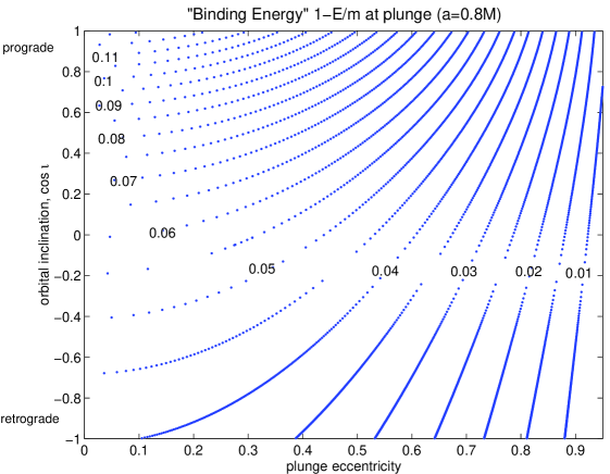
FIG. 1.: “Specific binding energy”, $1-E/m$, at plunge, as a function of the plunge eccentricity and inclination angle, for a Kerr BH with spin parameter $a=0.8M$. The quantity $1-E/m$ approximates $\alpha$—the amount of energy (per CO’s mass $m$) emitted to infinity in GWs during the entire inspiral. For the case $a=0.8M$ shown here, and for astrophysically relevant inspirals with $e_{\rm LSO}\mathrel{\hbox{\hbox to0.0pt{\hbox{\lower 4.0pt\hbox{$\sim$}}\hss}\hbox{$<$}}}0.35$, the CO emits between $\sim 4\%$ and $\sim 12\%$ of its mass in GWs (the former value for retrograde, the latter for prograde equatorial orbits).

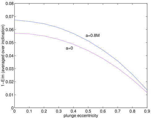
FIG. 2.: Specific binding energy at plunge, averaged over (uniformly distributed) inclination angles, as a function of the plunge eccentricity. The plot compares the case $a=0.8$ of Fig. 1, with the case of a non-spinning MBH ($a/M=0$). In the latter case, the plunge energy is given by Eq. (10). An “inclination averaged” inspiral in the astrophysically relevant range of plunge eccentricities ($e_{\rm LSO}\mathrel{\hbox{\hbox to0.0pt{\hbox{\lower 4.0pt\hbox{$\sim$}}\hss}\hbox{$<$}}}0.35$), emits around 5–7% of the CO’s mass in GWs, with only little dependence on the MBH’s spin.

In the analysis below, we will adopt $\alpha=0.06$ as a fiducial average value, based on Fig. 2.

B GW energy spectrum from a single capture

Ideally, we would next compute the spectrum $f(dE/df)$ of GW energy emitted over the entire inspiral, for given values of $m$, $M$, $a$, $e_{LSO}$, and ${\iota}_{LSO}$. However, that would be a much harder problem than the one in Sec. III A. The tools to do a fully satisfactory job do not even exist yet, since there is still no working code to calculate the effect of GW radiation reaction on an arbitrary geodesic orbit in Kerr. Nevertheless, a reasonable job at approximating the orbital evolution could presumably be done today by inferring the rate of change of the CO’s $E$ and $L_{z}$ from the flux of energy and angular momentum at infinity, and approximating the orbital inclination angle $\iota$ as fixed during the inspiral (Hughes [10] discusses the justification of this approximation)—which determines the rate of change of $Q$. Knowing the orbital evolution, one could obtain the GW spectrum by solving the Teukolsky equation for the emitted GWs.

However, astronomical capture rates are sufficiently uncertain that we feel justified in a much cruder approach to this problem: We calculate the spectrum using the approximate, analytic formalism we previously developed in [8]. In this formalism, the overall orbit is imagined as osculating through a sequence of Keplerian orbits, with rate of change of energy, eccentricity, periastron direction, etc. determined by solving post-Newtonian evolution equations. In this approximation, the emitted waveform $h_{\mu\nu}(t)$, at any instant, is determined by applying the quadrupole formula to an instantaneous Keplerian orbit. The quadrupole-formula waveform for an eccentric, Keplerian orbit was derived analytically long ago by Peters and Matthews [13], so these approximate waveforms are relatively easy to calculate. These waveforms correctly capture the fact that eccentric orbits have power at all multiples of the orbital frequency (even when considering only quadrupole radiation, as we do). We “cut off” the waveform when the orbit reaches the point of plunge for a Schwarzschild MBH, at $r_{p}=(6+2e_{LSO})/(1+e_{LSO})$—thus, we are essentially restricting ourselves to the $a=0$ case. (This is partly because our post-Newtonian evolution equations cannot be trusted for prograde orbits in near-extremal Kerr. However, given the small difference between the $a=0$ and $a=0.8M$ cases in Fig. 2, and given that we will subsequently average the spectra over $M$, the restriction to $a=0$ here should not appreciably affect the final average spectrum.)

Figure 3 shows the spectrum of a single capture (for a range of possible plunge eccentricities), as derived from the approximate waveform model described above. For each value of $e_{\rm LSO}$ we integrated post-Newtonian evolution equations [Eqs. (28) and (30) in [8]] backward in time to obtain $e(t)$ and $\nu(t)$, and, consequently, $e(\nu)$. We then obtained the power radiated into each of the harmonics of the orbital frequency using the leading-order formula [13]

$$\dot{E}_{n}(\nu)=\frac{32}{5}\mu^{2}M^{4/3}(2\pi\nu)^{10/3}g_{n}[e(\nu)],$$ (11)

where $g_{n}(e)$ is given by

$$g_{n}(e) = \frac{n^{4}}{32}\bigl{\{}\bigl{[}J_{n-2}(ne)-2e\,J_{n-1}(ne)+\frac{2}{n}\,J_{n}(ne)+2e\,J_{n+1}(ne)-J_{n+2}(ne)\bigr{]}^{2}$$ (13)

$$+(1-e^{2})[J_{n-2}(ne)-2\,J_{n}(ne)+J_{n+2}(ne)]^{2}+\frac{4}{3n^{2}}[J_{n}(ne)]^{2}\bigr{\}}.$$

We next re-expressed $\dot{E}_{n}(\nu)$ in terms of the GW frequency $f$ by replacing $\nu\to f_{n}/n$ for each of the $n$-harmonics. Finally, we summed up the power from all harmonics (holding $f$ fixed), and plotted the total power vs. $f$. (In practice, we summed over the first $20$ harmonics. Note that different harmonics “cut off” at different GW frequency, $f_{\rm LSO}=n\,\nu_{\rm LSO}$, giving rise to the “discontinuities” apparent in Fig. 3.) During the inspiral the source evolves significantly in both frequency and eccentricity, with the GW power distribution shifting gradually from high harmonics of the orbital frequency to lower harmonics. This leads to a spectrum with a steep rise followed by a “plateau”, as manifested in the Figure. For comparison, a decaying, quasi-circular orbit would yield a simple power-law spectrum, $f(dE/df)\propto f^{2/3}$.

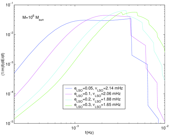
FIG. 3.: Energy spectrum of a single inspiral, for $M=10^{6}M_{\odot}$, $a=0$, and for a range of plunge eccentricities $e_{\rm LSO}$. $\nu_{\rm LSO}$ is the orbital frequency at the LSO. These spectra are based on approximate, post-Newtonian waveforms as described in the text. Each of the curves represents the sum of contributions from the first 20 harmonics of the orbital frequency. Discontinuities appear whenever an $n$-harmonic reaches frequency $n\times\nu_{\rm LSO}$ and cuts off.

C Model capture spectrum, averaged over $e_{\rm LSO}$

Ideally, the next step in our analyis would be to integrate the individual capture spectra over the actual distribution of final eccentricities, in order to obtain an appropriately weighted average. However, since that distribution is poorly known, and since our individual spectra are anyway approximated, we instead introduce the following model for the “average” spectrum (for a given MBH mass), suggested by Fig. 3:

$$f(dE/df)=m\times\left\{\begin{array}[]{ll}(f/f_{0})^{3},&f<f_{p},\\ {\rm const}=(f_{p}/f_{0})^{3},&f_{p}<f<4f_{p},\\ 0,&f>4f_{p}.\end{array}\right.$$ (14)

Here, $f_{0}$ is a normalization parameter we will determine soon, and $f_{p}$ is the plunge frequency at $e_{\rm LSO}=0$:

$$f_{p}=\left(2\pi 6^{3/2}M\right)^{-1}=2.20\,{\rm mHz}\times M_{6}^{-1},$$ (15)

where, recall, $M_{6}\equiv M/(10^{6}M_{\odot})$.

The parameter $f_{0}$ is determined from the total energy radiated in GWs over the entire inspiral. Let this total energy be $\alpha m$, where, recall, $\alpha$ is roughly our fiducial value of $0.06$. We have

$$\alpha=m^{-1}\int_{0}^{\infty}f(dE/df)d\ln f=\int_{0}^{f_{p}}(f/f_{0})^{3}df/f+\int_{f_{p}}^{4f_{p}}(f_{p}/f_{0})^{3}df/f=(f_{p}/f_{0})^{3}[1/3+\ln(4)],$$ (16)

and solving for $f_{0}$ yields

$$f_{0}=6.74\,{\rm mHz}\times(\alpha/0.06)^{-1/3}M_{6}^{-1}.$$ (17)

Thus the energy spectrum can be rewritten as

$$f(dE/df)=(m/M_{\odot})M_{\odot}\times(\alpha/0.06)\times\left\{\begin{array}[]{ll}3.27\times 10^{-3}M_{6}^{3}f_{\rm mHz}^{3},&f<f_{p},\\ 3.49\times 10^{-2},&f_{p}<f<4f_{p},\\ 0,&f>4f_{p}\,,\end{array}\right.$$ (18)

where $f_{\rm mHz}\equiv f/(1\,{\rm mHz})$. This spectrum is illustrated in Fig. 4. Our model spectrum is not particularly accurate, but it is good enough for our purposes: We will further average it over the MBH mass (in section III.B.), and the result of this averaging will anyway “smear out” the exact details of the shape shown in Fig. 4. For our application, what matters most is that our model spectrum is peaked at roughly the right frequency, $f\sim 5\,{\rm Hz}/M_{6}$, that it is relatively narrow (most of the energy is contained within a factor $\sim 5-10$ range in frequency), and that it “contains” the right total amount of energy.

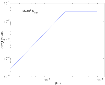
FIG. 4.: Our model spectrum [Eq. (18)] for a single inspiral with $M=10^{6}M_{\odot}$, averaged over inclination angle and final eccentricity, and normalized to $\alpha=0.06$. The $n^{th}$ GW harmonic cuts off when $f/n$ reaches the plunge frequency, $f_{p}$, causing the spectrum to flatten out for $f_{p}\mathrel{\hbox{\hbox to0.0pt{\hbox{\lower 4.0pt\hbox{$\sim$}}\hss}\hbox{$<$}}}f\mathrel{\hbox{\hbox to0.0pt{\hbox{\lower 4.0pt\hbox{$\sim$}}\hss}\hbox{$<$}}}4f_{p}$. We cut off our model spectrum at $f>4f_{p}$, where we no longer find emission from any of the dominant harmonics ($n\sim 2-4$).

D Model capture spectrum, averaged over MBH mass

The above model spectrum corresponds to a given MBH mass $M$. We next average this spectrum over $M$, with the average being weighted by the capture rate for MBHs of mass $M$.

From Eq. (2), the (current) rate of captures by MBHs of mass $M$ is $\propto M^{3/8}$. The space number density of MBHs with masses $0.1\mathrel{\hbox{\hbox to0.0pt{\hbox{\lower 4.0pt\hbox{$\sim$}}\hss}\hbox{$<$}}}M_{6}<10$ is approximately constant in this range [see Eq. (1)]. Therefore, the average GW energy spectrum from a single capture (per unit mass of the CO) is approximately

$$\epsilon(f)=0.1923\,(\alpha/0.06)\,\int_{0.1}^{10}(dM_{6}/M_{6})M_{6}^{3/8}\times\left\{\begin{array}[]{ll}3.27\times 10^{-3}M_{6}^{3}f_{\rm mHz}^{3},&f<f_{p},\\ 3.49\times 10^{-2},&f_{p}<f<4f_{p},\\ 0,&f>4f_{p},\end{array}\right.$$ (19)

where $f_{p}\equiv f_{p}(M_{6})$ is given in Eq. (15), and the prefactor 0.1923 is just $[\int_{0.1}^{10}(dM_{6}/M_{6})M_{6}^{3/8}]^{-1}$.

To evaluate the integral in Eq. (19) we consider separately 5 different frequency ranges:
For $\mathbf{f<0.22}$ mHz we have $f<f_{p}$ for any $M$ in the integration domain. This low-frequency range is therefore controlled by the “tail” part of the spectrum, and we find

$$\epsilon(f<0.22\,{\rm mHz}) = (\alpha/0.06)\,6.297\times 10^{-4}f_{\rm mHz}^{3}\int_{0.1}^{10}dM_{6}M_{6}^{19/8}$$ (20)

$$= (\alpha/0.06)\,4.425\times 10^{-1}f_{\rm mHz}^{3}\,.$$ (21)

For $\mathbf{0.22<f<0.88}$ mHz we have $f<4f_{p}$ for any $M$, and now there are both “tail” and “plateau” contributions:

$$\epsilon(0.22<f<0.88\,{\rm mHz}) = (\alpha/0.06)\left[6.297\times 10^{-4}f_{\rm mHz}^{3}\int_{0.1}^{2.2/f_{\rm mHz}}M_{6}^{19/8}dM_{6}+6.710\times 10^{-3}\int_{2.2/f_{\rm mHz}}^{10}M^{-5/8}dM_{6}\right]$$ (22)

$$= (\alpha/0.06)\,4.243\times 10^{-2}(1-0.5039\,f_{\rm mHz}^{-3/8}).$$ (23)

For $\mathbf{0.88<f<22}$ mHz we need to cut off the integration at $M_{6}=8.8\,{\rm mHz}/f$:

$$\epsilon(0.88<f<22\,{\rm mHz}) = (\alpha/0.06)\left[6.297\times 10^{-4}f_{\rm mHz}^{3}\int_{0.1}^{2.2/f_{\rm mHz}}M_{6}^{19/8}dM_{6}+6.710\times 10^{-3}\int_{2.2/f_{\rm mHz}}^{8.8/f_{\rm mHz}}M^{-5/8}dM_{6}\right]$$ (24)

$$= (\alpha/0.06)(1.907\times 10^{-2}f_{\rm mHz}^{-3/8}-7.881\times 10^{-8}f_{\rm mHz}^{3}).$$ (25)

For $\mathbf{22<f<88}$ mHz there remains only a plateau contribution:

$$\epsilon(22<f<88\,{\rm mHz}) = (\alpha/0.06)6.710\times 10^{-3}\int_{0.1}^{8.8/f_{\rm mHz}}M^{-5/8}dM_{6}$$ (26)

$$= (\alpha/0.06)\,4.046\times 10^{-2}(f_{\rm mHz}^{-3/8}-0.1866).$$ (27)

Lastly, we have

$$\epsilon(f>88\,{\rm mHz})=0.$$ (28)

To summarize, the energy spectrum from captures (per unit CO mass), averaged over all captures by MBHs with masses in the range $10^{5}$ to $10^{7}M_{\odot}$, is

$$\epsilon(f)=(\alpha/0.06)\times\left\{\begin{array}[]{ll}4.425\times 10^{-1}f_{\rm mHz}^{3},&f_{\rm mHz}<0.22,\\ 4.243\times 10^{-2}(1-0.5039\,f_{\rm mHz}^{-3/8}),&0.22<f_{\rm mHz}<0.88,\\ 1.907\times 10^{-2}f_{\rm mHz}^{-3/8}-7.881\times 10^{-8}f_{\rm mHz}^{3},&0.88<f_{\rm mHz}>22,\\ 4.046\times 10^{-2}(f_{\rm mHz}^{-3/8}-0.1866),&22<f_{\rm mHz}<88,\\ 0,&f_{\rm mHz}>88\,.\end{array}\right.$$ (29)

This spectrum is depicted in Fig. 5.

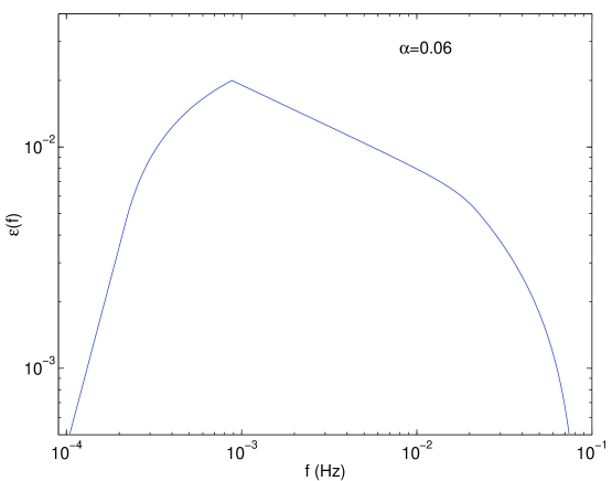
FIG. 5.: Model energy spectrum for a single capture, averaged over MBH mass and normalized by $\alpha=0.06$—see Eq. (29). Note the apparent sharp drops in the spectrum at frequencies below $\sim 10^{-3}$ Hz and above $\sim 2\times 10^{-2}$ Hz are simply an artifact of our restricting attention to MBH masses in the range $10^{5}-10^{7}M_{\odot}$.

IV Spectral density of capture background

A Total energy spectrum of capture background

Using the above estimates, we want to determine the ambient GW spectrum from all captures in the history of the universe. To simplify the analysis, we will first assume that spacetime is flat, that the capture rate has been fixed at ${\cal R}^{A}(0)$ for the last $T=\beta\cdot 10^{10}$ years, and that previous to that the capture rate had been zero. In Subsection IV D below we carry out a more careful analysis, including cosmological and evolutionary effects, and show that the above simplified version actually gives reasonably accurate results, especially if one makes the judicious choice $\beta=0.7$.

Using our flat spacetime assumptions, the GW energy density spectrum from captures of species A, $d\rho^{A}_{\rm GW}/d({\rm ln}f)$, is just the average energy spectrum per capture, $m^{A}\epsilon(f)$, times the current total capture rate per unit co-moving volume, ${\cal R}^{A}(0)$, times $T$. From Eqs. (1) and (2), the factor ${\cal R}^{A}(0)$ is

$${\cal R}^{A}(0) = \int_{0.1}^{10}{\cal R}^{A}(M;0)(dN/dM_{6})dM_{6}$$ (30)

$$= 1.040\,(\kappa^{A}/10^{-7})\,\gamma\,h_{70}^{2}\,{\rm Gpc}^{-3}{\rm yr}^{-1}\,.$$ (31)

Using $d\rho^{A}_{\rm GW}/d({\rm ln}f)=m^{A}{\cal R}^{A}(0)T\,\epsilon(f)$, with the conversion factor $1M_{\odot}/{\rm Gpc}^{3}=4.521\times 10^{-57}\ {\rm s}^{-2}$ , we then find

$$\frac{d\rho^{A}_{\rm GW}}{d({\rm ln}f)}=3.291\times 10^{-47}\left(\frac{m^{A}}{M_{\odot}}\right)\left(\frac{\beta}{0.7}\right)\left(\frac{\kappa^{A}}{10^{-7}}\right)\,\gamma\,h_{70}^{2}\times\epsilon(f)\ {\rm sec}^{-2},$$ (32)

where, recall, $\epsilon(f)$ is given in Eq. (29) above.

B LISA noise model

Our estimate of $d\rho^{A}_{\rm GW}/d({\rm ln}f)$ leads directly to an estimate of the spectral density of the capture background measured by the LISA detector. But before proceeding to this, we briefly state our conventions and review standard estimates for the magnitudes of other noise sources. For more details we refer the reader to Sec. V.A of Ref. [8].

LISA’s GW data stream is basically equivalent to the output of two synthesized Michelson interferometers, where in each Michelson the angle between the two arms is $60^{\circ}$, and where the two Michelsons—hereafter labelled I and II— are rotated with respect to each other by $45^{\circ}$. This representation is only accurate for low frequencies, $f\mathrel{\hbox{\hbox to0.0pt{\hbox{\lower 4.0pt\hbox{$\sim$}}\hss}\hbox{$<$}}}0.01$ Hz. However, most of the SNR from captures will indeed be accumulated at these lower frequencies, so this approximation is adequate for our purpose. At low $f$, our synthesized detectors I and II are basically equivalent to the data combinations lablelled A and E in the terminology of Time Delay Interferometry [14]. The output $s_{I}(t)$ of synthetic-Michelson I is the sum of resolvable GW signals $h_{I}(t)$ and noise $n_{I}(t)$; similarly, $s_{II}(t)=n_{II}(t)+h_{II}(t)$.

In keeping with the usual convention in the LISA literature, we define $S_{h}(f)$ to be the single-sided, sky-averaged noise spectral density for either synthetic detector, I or II:

$$\langle{\tilde{n}_{I}}(f)\,{\tilde{n}_{I}}(f^{\prime})^{*}\rangle=\langle{\tilde{n}_{II}}(f)\,{\tilde{n}_{II}}(f^{\prime})^{*}\rangle={3\over 40}\delta(f-f^{\prime})S_{h}(f),$$ (33)

where a tilde denotes the Fourier transform and “$\langle\ \rangle$” stands for the expectation value. The factor ${3\over 40}$ here is the product of the following three factors: ${1\over 2}$ from the “single-sided” convention, ${3\over 4}={\rm sin}^{2}60^{\circ}$ because the angle between the arms is $60^{\circ}$, and ${1\over 5}$ from an average over source directions and polarizations. [Note here we are using a different convention than in our earlier paper [8], where $S_{h}(f)$ was defined without the sky-averaging factor.]

LISA’s noise has three main components (besides confusion noise from captures): instrumental noise, confusion noise from short-period galactic binaries (mostly WD binaries), and confusion noise from short-period extragalactic binaries. For LISA’s instrumental noise, $S^{\rm inst}_{h}(f)$, we use the curve available from S. Larson’s online sensitivity curve generator [15], which is based on the noise budgets specified in the LISA Pre-Phase A Report [16]. For $f\mathrel{\hbox{\hbox to0.0pt{\hbox{\lower 4.0pt\hbox{$\sim$}}\hss}\hbox{$<$}}}5$ mHz, the instrumental noise curve is well fitted analytically by [17]

$$S^{\rm inst}_{h}(f)=6.12\times 10^{-51}f^{-4}+1.06\times 10^{-40}+6.12\times 10^{-37}f^{2}\ {\rm Hz}^{-1},$$ (34)

where $f$ is in Hz.

Next we turn to confusion noise from galactic and extragalactic WD binaries (GWDBs and EGWDBs, respectively). Any isotropic background of individually unresolvable GW sources represents (for the purpose of analyzing other sources) a noise source with spectral density [18] 

$${\cal S}^{\rm backgd}_{h}(f)=\,\frac{4}{\pi}f^{-3}\frac{d\rho_{\rm GW}}{d({\rm ln}f)}\,.$$ (35)

Here and throughout this paper, our convention is to use the “calligraphic” ${\cal S}_{h}$ to represent the spectral density of the entire background from some class of sources, including both resolvable and unresolvable sources. The fraction of ${\cal S}_{h}$ due to the unresolvable sources, which we refer to as “confusion noise”, we denote by $S_{h}$ with an Italic typeface. We shall also use the “upright” typeface for the instrumental noise, $S^{\rm inst}_{h}$. Estimates of $d\rho_{\rm GW}/d\ln f$ from the galactic and extragalactic WD backgrounds [19, 20] then yield the following background spectral densities:

$${\cal S}^{\rm GWDB}_{h}(f) = 1.4\times 10^{-44}\,\left(\frac{f}{1{\rm Hz}}\right)^{-7/3}{\rm Hz}^{-1},$$ (36)

$${\cal S}_{h}^{\rm EGWDB}(f) = 2.8\times 10^{-46}\left(\frac{f}{1{\rm Hz}}\right)^{-7/3}{\rm Hz}^{-1}.$$ (37)

(In fact, there is practically no distinction between ${\cal S}_{h}^{\rm EGWDB}$ and $S_{h}^{\rm EGWDB}$, since the entire extragalactic contribution is assumed to consist of unresolvable sources.)

The GWDB background is actually larger than LISA’s instrumental noise in the range $\sim 10^{-4}$–$10^{-2}$ Hz. However, at frequencies $f\gtrsim 2\times 10^{-3}\,$Hz, galactic sources are sufficiently sparse, in frequency space, that one expects to be able to “fit them out” of the data. Still, even resolvable sources introduce an additional kind of “noise” since they can never be subtracted out perfectly. To the extent that such “subtraction errors” can together mimic other classes of astrophysically interesting signals, they effectively diminish the sensitivity of LISA to those other signals. (This effect is also referred to simply as “confusion noise” within the LISA community, though conceptually it can be useful to consider the two kinds of confusion noise separately.) In the case of GWDBs at frequencies above $\mathrel{\hbox{\hbox to0.0pt{\hbox{\lower 4.0pt\hbox{$\sim$}}\hss}\hbox{$>$}}}2$mHz (i.e., at frequencies where they become individually resolvable), this second type of confusion noise acts effectively like a multiplicative factor on all other types of noise. E.g., if one is searching for coalescing MBH binaries, but the signal from some fraction $F(f)$ of the frequency bins near frequency $f$ are rendered effectively unusable for this purpose because of degeneracies with the fitted GWDBs, then it is as if the noise spectral density were increased by a factor $(1-F)^{-1}$ [21].

We denote by $S^{\rm eff}_{h}$ the total effective noise, including the multiplicative effect from this second type of confusion noise, and adopt the following rough estimate of $S^{\rm eff}_{h}$, based on Hughes [22]:

$$S^{\rm eff}_{h}(f)={\rm min}\left\{\left[S_{h}^{\rm inst}(f)+{\cal S}_{h}^{\rm EGWDB}(f)\right]\exp(\kappa T_{\rm mission}^{-1}dN/df),\;\;S_{h}^{\rm inst}(f)+{\cal S}_{h}^{\rm EGWDB}(f)+{\cal S}_{h}^{\rm GWDB}(f)\right\}\,.$$ (38)

Here $dN/df$ is the number density of GWDBs per unit GW frequency, $T_{\rm mission}$ is the LISA mission lifetime (so $\Delta f=1/T_{\rm mission}$ is the bin size of the discretely Fourier transformed data), and $\kappa$ is the average number of frequency bins that are “lost” (for the purpose of analyzing other sources) when each galactic binary is fitted out. For $dN/df$ we adopt the estimate [22]

$${dN\over df}=2\times 10^{-3}\,{\rm Hz}^{-1}\left(1\,{\rm Hz}\over f\right)^{11/3},$$ (39)

and take $\kappa T_{\rm mission}^{-1}=1.5/{\rm yr}$ (corresponding, e.g., to $T_{\rm mission}\approx 3\,$yr and $\kappa\approx 4.5$).

Even though the subtracted noise model, Eq. (38), basically represents an “educated guess,” it has the right qualitative features: The very steep slope of $dN/df$ means that a factor $3$ increase in $f$ is sufficient to reduce the source density from (say) $7/$bin to $1/(8\ {\rm bins})$. The “unsubtractable part” of the galactic WD curve must therefore fall very steeply near $f\sim 1-2$ mHz—a feature accounted for by the exponential function in Eq. (38). Also, a factor (say) $2$ change in our fiducial value for $\kappa T_{\rm mission}^{-1}$ would only shift the “drop-off” frequency by a factor $2^{3/11}\approx 1.2$. Therefore we believe Eq. (38) must be a reasonably accurate representation of the total effective noise.

There are likely tens of thousands of CO capture sources (out to $z=1$) in the LISA band at any instant, and we shall see that a signficant fraction of them are not resolvable. How should we modify Eq. (38) to take into account confusion noise from CO captures? We shall see that even if all CO captures were unsubtractable, so that the entire capture background is “counted” as confusion noise, the CO confusion noise would still be smaller than the (pre-subtraction) noise from GWDBs, though it could be larger than the instrumental noise (depending on the exact capture rates). In this case, it seems sensible, as a first approximation, to simply add the CO confusion noise contribution, $S_{h}^{\rm capt}(f)$, to $S_{h}^{\rm inst}(f)$ in Eq. (38). That is, we estimate the total effective noise density as

$$S^{\rm eff}_{h}(f) = {\rm min}\left\{\left[S_{h}^{\rm inst}(f)+S_{h}^{\rm EGWDB}(f)+S_{h}^{\rm capt}(f)\right]\exp(\kappa T^{-1}dN/df),\right.$$ (41)

$$\quad\quad\quad\left.S_{h}^{\rm inst}(f)+{\cal S}_{h}^{\rm GWDB}(f)+S_{h}^{\rm EGWDB}(f)+S_{h}^{\rm capt}(f)\right\}.$$

Note that Eq. (41) does not include the effect of “subtraction errors” made in removing the resolvable CO captures. We can reasonably neglect this noise contribution, for the following reason. Over a $\sim 3-$yr mission, the number of individually detected captures will probably be $\mathrel{\hbox{\hbox to0.0pt{\hbox{\lower 4.0pt\hbox{$\sim$}}\hss}\hbox{$<$}}}3\times 10^{3}$ [1]. Each capture source is completely specified by $17$ parameters [8]; thus $\sim 5\times 10^{4}$ real numbers are required to specify their combined signal. In comparison, the signal (from both synthetic detectors) between $1$ and $10$ mHz is represented by $\sim 4\times 10^{6}$ real numbers (i.e., roughly $10^{6}$ discrete frequency bins, times two real numbers per bin, times two independent detectors), so in principle only $\sim 1\%$ of the available bandwidth is “lost” by fitting out these captures.

C Noise spectral density

We now obtain ${\cal S}^{\rm Acapt}_{h}(f)$—the spectrum of the background from all capture sources of type A—by simply combining Eqs. (29), (32), and (35). This yields

$${\cal S}^{\rm Acapt}_{h}(f) = 10^{-39}\ {\rm Hz}^{-1}\left(\frac{m^{A}}{M_{\odot}}\right)\left(\frac{\alpha}{0.06}\right)\left(\frac{\beta}{0.7}\right)\left(\frac{\kappa^{A}}{10^{-7}}\right)\,\gamma\,h_{70}^{2}$$ (48)

$$\times\left\{\begin{array}[]{ll}18.540&f_{\rm mHz}<0.22,\\ 1.778f^{-3}_{\rm mHz}(1-0.5039\,f_{\rm mHz}^{-3/8}),&0.22<f_{\rm mHz}<0.88,\\ 0.799f_{\rm mHz}^{-27/8}-3.302\times 10^{-6},&0.88<f_{\rm mHz}<22,\\ 1.695f^{-3}_{\rm mHz}(f_{\rm mHz}^{-3/8}-0.1866),&22<f_{\rm mHz}<88,\\ 0,&f_{\rm mHz}>88.\end{array}\right.\$$

Recall that here $\alpha$ is the total amount of energy (per CO’s mass $m$) radiated over the course of a single inspiral (cf. Fig. 2), $\beta$ is the time (in units of $10^{10}$ yr) during which captures occur, $\kappa^{A}$ is an event rate parameter [see Eq. (4)], and $\gamma$ is a parameter of order unity that normalizes the space-density of MBHs. This capture background is plotted in Figs. 6, 7, and 8 (for captures of WDs, NSs, and BHs, respectively), superposed on LISA’s instrumental noise and WD-binaries confusion noise. Each of these figures plots the background for a range of assumed capture rates $\kappa^{A}$; the other parameters in Eq. (48) are all assumed to have their fiducial values: $\alpha=0.06$, $\beta=0.7$, and $\gamma=1.0$. The WD, NS, and BH masses are $0.6,1.4$, and $10M_{\odot}$, respectively.

FIG. 6.: Comparison of the background ${\cal S}_{h}^{\rm WDcapt}$ from all WD captures (dash-dot lines) with LISA’s instrumental noise (solid line) and with LISA’s instrumental plus confusion noise from WD binaries (dashed line). We show three cases, corresponding to WD capture rates of $\kappa^{\rm WD}=4\times 10^{-6},4\times 10^{-7}$, and $4\times 10^{-8}$—cf. Eqs. (2) and (3).

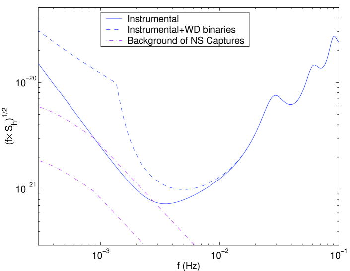
FIG. 7.: Same as in Fig. 6, but this time showing the background ${\cal S}_{h}^{\rm NScapt}$ from all NS captures. We show two cases, corresponding to NS capture rates of $\kappa^{\rm NS}=6\times 10^{-7}$ and $6\times 10^{-8}$.

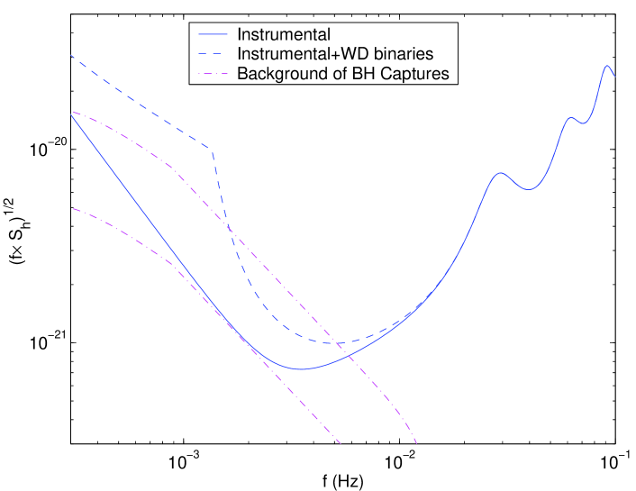
FIG. 8.: Same as in Fig. 6, but this time showing the background ${\cal S}_{h}^{\rm BHcapt}$ from all BH captures. We show two cases, corresponding to BH capture rates of $\kappa^{\rm BH}=6\times 10^{-7}$ and $6\times 10^{-8}$.

D Influence of cosmology and source evolution

Our calculation of ${\cal S}_{h}^{\rm capt}(f)$ in the previous subsection ignored source evolution and treated the spacetime as flat—counting all sources within $\beta\times 10^{10}$ lt-yr of us and ignoring the rest. Here we repeat the calculation but for a realistic cosmology and a few different evolutionary scenarios. We shall see that if we set $\beta$ to $0.7$, then in the crucial $1-5\,$Hz range (where capture noise could possibly have a significant impact on LISA’s total effect noise level), this more-accurate treatment results in differences from our flat model at a level $\mathrel{\hbox{\hbox to0.0pt{\hbox{\lower 4.0pt\hbox{$\sim$}}\hss}\hbox{$<$}}}15\%$. This uncertainty associated with source evolution is still much smaller than the uncertainty in the current event rate.

Let $\dot{\cal E}(f,z)\Delta f$ be the rate (per unit proper time, per unit co-moving volume) at which GW energy between frequencies $f$ and $f+\Delta f$ is emitted into the universe, at red-shift $z$. (Here $f$ is the frequency measured by a contemporaneous observer, not the red-shifted frequency we measure today.) For instance, for source type A, the rate today is $\dot{\cal E}(f,0)={\cal R}^{A}(0)m^{A}f\epsilon(f)$. The dependence of $\dot{\cal E}(f,z)$ on $z$ arises principally from two effects. Firstly, the capture rate in the past, ${\cal R}^{A}(M;z)$ (measured per unit proper time, per MBH) can differ from today’s rate ${\cal R}^{A}(M;0)$. Secondly, the MBHs were smaller in the past (since they are growing by accretion), which implies that the spectrum $\dot{\cal E}(f,z=2)$ (say) is blue-shifted compared to the spectrum $\dot{\cal E}(f,z=0)$. (We stress that this blue-shifting is a source-evolution effect. There is also a cosmological red-shift, to be accounted for momentarily.) The total number of MBHs (per unit comoving volume) may also evolve due to mergers, but we expect this effect to be small between $z\mathrel{\hbox{\hbox to0.0pt{\hbox{\lower 4.0pt\hbox{$\sim$}}\hss}\hbox{$<$}}}2$ and now, and so for simplicity we take this total number to be constant.

To calculate the GW energy density today, in some frequency band of width $\Delta f$, one integrates the contributions from all times, after appropriate red-shifting of the waves’ frequency and energy:

$$\frac{d\rho}{df}\Delta f=\int_{z_{\rm max}}^{0}\frac{\dot{\cal E}[f(1+z),z]}{1+z}\Delta f^{\prime}\frac{d\tau}{dz}dz,$$ (49)

where $\Delta f^{\prime}=\Delta f(1+z)$ is the blue-shifted (relative to today) frequency range of the GWs when initially emitted, and the factor $1+z$ in the denominator accounts for the decrease in the waves’ energy due to the redshift between $z$ and now. Obviously the two $(1+z)$ factors cancel, so Eq. (49) can be simplied to [23, 24]

$$\frac{d\rho}{df}=\int_{z_{\rm max}}^{0}\dot{\cal E}[f(1+z),z]\frac{d\tau}{dz}dz.$$ (50)

We shall assume a spatially flat $(\Omega=1.0$) Friedman-Lema$\hat{\rm i}$tre-Robertson-Walker universe, with $\Omega_{\Lambda}=0.70$ and $\Omega_{m}=0.30$. For our fiducial cosmology, the universe’s current age $\tau_{0}$ is given by

$$\tau_{0}=0.964H_{0}^{-1}=1.39\times 10^{10}h_{70}^{-1}\ {\rm yr}.$$ (51)

Here we shall consider only sources in the range $0<z<2$. (We will see below that sources at $z>2$ are unlikely to add considerably to $\rho_{\rm GW}$.) In this range, the following power law relation between the universe’s age $\tau$ and redshift $z$ is accurate to within $\sim 3\%$:

$$\tau=\tau_{0}(1+z)^{-1.18}\,.$$ (52)

For our estimates in this section, we will approximate this as $\tau=\tau_{0}(1+z)^{-1.2}$.

To get some idea for the range of possible answers, we shall consider two possible scalings for the capture rates ${\cal R}^{A}(z)$ and two possible scalings for the MBH mass $M(z)$ (i.e., four possible scenarios in all): For the capture rates, simulations of Milky Way captures by Freitag [6], as well as an analytic argument by Phinney [25], both suggest that ${\cal R}^{A}(z)$ should increase in the past like $\tau^{-1/2}\propto(1+z)^{0.6}$. For comparison, we will also consider an ${\cal R}^{A}(z)={\rm const}$ scenario. Similarly, for the MBH masses, we will consider as possibilities (i) $M={\rm const}$ and (ii) $M\propto\tau^{1/2}$ (as suggested by Sirota et al. [26]). The four different assumptions yield the following four different relations between $\dot{\cal E}(f,z)$ and $\dot{\cal E}(f,0)$:

$$\dot{\cal E}(f,z) = \left\{\begin{array}[]{ll}\dot{\cal E}(f,0),&{\cal R}^{A}(z)={\rm const},\,M={\rm const},\\ (1+z)^{0.6}\,\dot{\cal E}(f,0),&{\cal R}^{A}(z)\propto(1+z)^{0.6},\,M={\rm const},\\ (1+z)^{-0.6}\,\dot{\cal E}[f(1+z)^{-0.6},0],&{\cal R}^{A}(z)={\rm const},\,M\propto(1+z)^{-0.6},\\ \dot{\cal E}[f(1+z)^{-0.6},0]&{\cal R}^{A}(z)\propto(1+z)^{0.6},\,M\propto(1+z)^{-0.6}.\end{array}\right.\$$ (57)

To derive the third line on the RHS, note that under a rescaling of MBH mass, $M\rightarrow M^{\prime}=\lambda M$, with total luminosity fixed, the spectrum gets re-scaled according to $\dot{\cal E}^{\prime}(f^{\prime})\Delta f^{\prime}=\dot{\cal E}(f)\Delta f$, where $f^{\prime}=\lambda^{-1}f$, or

$$\dot{\cal E}^{\prime}(f^{\prime})=\lambda\,\dot{\cal E}(\lambda f^{\prime})\,.$$ (58)

In our case, $M^{\prime}$ is the MBH mass at redshift $z$, so $\lambda=(1+z)^{-0.6}$, and the third line follows when we replace the dummy variable $f^{\prime}$ by $f$. Lines 2 and 4 on the RHS of Eq. (57) are obtained by simply multiplying lines 1 and 3 (respectively) by $(1+z)^{0.6}$ (the assumed rate enhancement factor for early times).

Again, we are interested in the CO capture spectrum chiefly in the range $1\mathrel{\hbox{\hbox to0.0pt{\hbox{\lower 4.0pt\hbox{$\sim$}}\hss}\hbox{$<$}}}f\mathrel{\hbox{\hbox to0.0pt{\hbox{\lower 4.0pt\hbox{$\sim$}}\hss}\hbox{$<$}}}7$ mHz. If we are to integrate Eq. (50) out to $z=2$ then we must know $\dot{\cal E}(f,0)$ for $f$ between $1$ mHz and $7\times(1+2)=21$ mHz. In this range, $\dot{\cal E}(f,0)$ is basically a power law: $\dot{\cal E}(f,0)\propto f^{-1}\epsilon(f)\propto f^{-11/8}$ (see Fig. 5).

For the remainder of this section, we will approximate $\dot{\cal E}(f,0)$ by the above simple power law; i.e., we assume $\dot{\cal E}(f,0)=W\,f^{-11/8}$ for some $W$. Using $d\tau/dz=-1.2\tau_{0}(1+z)^{-2.2}$ and integrating Eq. (50) out to $z=2$, we then obtain

$$\frac{d\rho}{df}=1.2\,\tau_{0}\,W\,f^{-11/8}\int_{1}^{3}{y^{-3.575+\mu+\sigma}dy},$$ (59)

where $y\equiv(1+z)$. In the exponent, $\mu=0$ [for $R^{A}(z)=R^{A}(0)$] or $0.6$ [for $R^{A}(z)=(1+z)^{0.6}R^{A}(0)$], and $\sigma=0$ [for $M(z)=M(0)$] or $(-0.6)(-11/8+1)=0.225$ [for $M(z)=M(0)(1+z)^{-0.6}$]. Note that the shape of the spectrum is always the same; only the amplitude varies with evolutionary scenario. We can write the result in the form

$$\frac{d\rho}{df}=W\,\tau_{\rm eff}\,f^{-11/8},$$ (60)

for some “effective” integration time $\tau_{\rm eff}$. Performing the elementary integral in Eq. (59) (taking $h_{70}=1$), we find for our 4 cases: $\tau_{\rm eff}=6.1\times 10^{9}$yr ($\mu=\sigma=0$), $\tau_{\rm eff}=7.5\times 10^{9}$yr ($\mu=0.6,\sigma=0$), $\tau_{\rm eff}=6.6\times 10^{9}$yr ($\mu=0,\sigma=0.225$), and $\tau_{\rm eff}=8.1\times 10^{9}$yr ($\mu=0.6,\sigma=0.225$).

By comparison, $\tau_{\rm eff}$ for the flat-universe/no-evolution model considered in the previous subsection would just be the total integration time: $\beta\times 10^{10}$yr. Thus, if we make the choice $\beta=0.7$, our flat-universe/no-evolution calculation agrees with all four of our cosmological/evolutionary models to within $\sim 15\%$. We note that $7\times 10^{9}$ years ago corresponds to $z=0.79$. We also note that in all four models, most of the contribution to the integral comes from the range $0<z<1$; the contribution from $1<z<2$ accounts for only $12-18\%$ of the total (depending on the case). This justifies our cutting off the integral at $z=2$, which is convenient, since our simple evolutionary models would not be trustworthy at higher $z$.

V Confusion noise from captures

In Sec. IV we estimated ${\cal S}^{\rm capt}_{h}(f)$, the spectrum of the background due to all captures. At $f=3$ mHz (i.e., near the bottom of LISA noise curve) ${\cal S}^{\rm capt}_{h}(f)$ equals the instrumental noise level $S^{\rm inst}_{h}(f)$ for $\kappa^{\rm WD}=1.6\times 10^{-6}$, $\kappa^{\rm NS}=6.8\times 10^{-7}$, or $\kappa^{\rm BH}=9.5\times 10^{-8}$. At the high end of their estimated ranges, the actual rates are larger than these values by factors of $\sim 2.5$, $1$, and $6$, respectively. Thus, confusion noise from capture sources could have a significant effect on the total LISA noise level, making it is important to next consider what fraction of ${\cal S}^{\rm capt}_{h}(f)$ actually constitutes an unresolvable confusion background (or, equivalently, what portion is resolvable and hence subtractable). With this goal in mind, we first make some general remarks on how the confusion noise level depends on both the event rate and the available subtraction method.

A General scalings of source rate, detection rate, and confusion noise

In this subsection, we step back and discuss the general phenomenon of confusion noise in GW searches. Consider some class $\cal C$ of astronomical sources, having some event rate $\cal R$, measured in ${\rm Mpc^{-3}yr^{-1}}$. (For sources that are always “on”, e.g. GWDBs, we would define $\cal R$ as just the spatial density, measured in ${\rm Mpc^{-3}}$.) We first ask: How does the detection rate $\cal D$ vary with $\cal R$? Here, for simplicity, we will imagine that source types other than $\cal C$ contribute negligibly to confusion noise; i.e., all noise is either instrumental noise or confusion noise from $\cal C$-type sources. Then for sufficiently low $\cal R$, confusion noise will be negligible, so the average distance $d_{\rm det}$ out to which one can detect individual $\cal C$-type sources is a constant (i.e., independent of $\cal R$) set by the instrumental noise level. Clearly, then, the detection rate $\cal D$ clearly grows linearly with $\cal R$ at small $\cal R$. But as one increases $\cal R$, eventually one must reach a point where confusion noise from $\cal C$-type sources dominates over the instrumental noise, and so determines $d_{\rm det}$. Clearly, for sufficiently large $\cal R$, almost all events add to the confusion noise, so $S_{h}^{\cal C}(f)\propto{\cal R}$, and therefore $d_{\rm det}\propto{\cal R}^{-1/2}$. If $d_{\rm det}$ is in the regime where space can be approximated as Euclidean and the source distribution can be approximated as spherically symmetric (generally true when $d_{\rm det}$ is much larger than typical separations between galaxies, but much smaller than a Hubble length: roughly $10{\rm Mpc}<d_{\rm det}<1{\rm Gpc}$), then the detection rate ${\cal D}\propto{\cal R}d_{\rm det}^{3}\propto{\cal R}^{-1/2}$, for large ${\cal R}$. Thus the individual-source detection rate $\cal D$ must peak at a certain rate ${\cal R}_{c}$, which is roughly the event rate at which confusion noise starts to dominate over instrumental noise in setting $d_{\rm det}$. This is illustrated in Fig. 9.

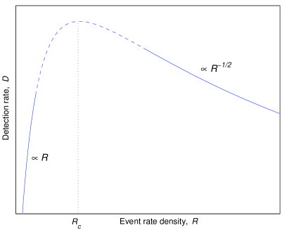
FIG. 9.: Illustration of how the detection rate $\cal D$ for some source class $\cal C$ scales with the event rate $\cal R$ (number of sources per unit time per unit space volume). For sufficiently small $\cal R$, we have ${\cal D}\propto{\cal R}$, whereas for very large $\cal R$ we have ${\cal D}\propto{\cal R}^{-1/2}$. Hence, the detection rate must peak at a certain event rate, ${\cal R}_{c}$. ${\cal R}_{c}$ is roughly the rate where confusion noise from $\cal C$-type sources begins to dominate the total noise level.

Next, we ask how the confusion noise $S_{h}^{\cal C}(f)$ from unresolvable sources scales with the rate ${\cal R}$. For low values of ${\cal R}$, $S_{h}^{\cal C}(f)$ should be a fixed fraction of ${\cal S}_{h}^{\cal C}(f)$ (arising from those sources whose SNR is too small to permit individual detection), and so grows linearly with $\cal R$. On the other hand, for very high ${\cal R}$, where confusion noise limits the detection rate, the fraction of source energy that is “unresolvable” grows and approaches one at sufficiently high ${\cal R}$; i.e., $S_{h}^{\cal C}(f)$ approaches ${\cal S}_{h}^{\cal C}(f)$. Thus, $S_{h}^{\cal C}(f)$ grows approximately linearly with ${\cal R}$ at very high ${\cal R}$, too, but with much larger slope than at low ${\cal R}$. Between these two regimes, near ${\cal R}_{c}$, $S_{h}^{\cal C}(f)$ grows nonlinearly with ${\cal R}$—see Fig. 10.

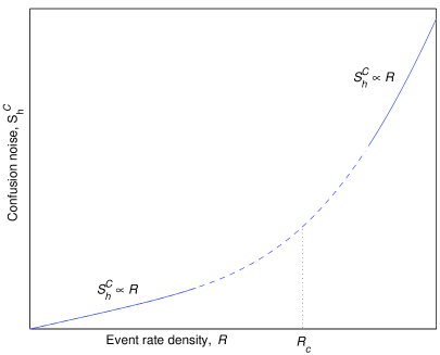
FIG. 10.: Illustration of how the confusion noise $S_{h}^{\cal C}$ scales with the event rate density $\cal R$. $S_{h}^{\cal C}$ is linear in $\cal R$ in both the very small $\cal R$ and very large $\cal R$ regimes. It depends on $\cal R$ non-linearly around the rate ${\cal R}_{c}$, where confusion noise begins to dominate the total noise level.

To recapitulate: First, we have observed that the event rate ${\cal R}$ where ${\cal S}_{h}^{\cal C}$ begins to dominate the total noise is roughly the event rate that gives the highest individual-source detection rate for ${\cal C}$-type sources—so one is lucky to be in that position! Second, the confusion noise level $S_{h}^{\cal C}$ is generally hardest to estimate precisely when it begins to dominate, since there it depends nonlinearly on ${\cal R}$. It is easy to see the problems that arise when $S_{h}^{\cal C}(f)$ vs. ${\cal R}$ is in the nonlinear regime: When confusion noise is the dominant noise source, one cannot determine which sources are detectable without first knowing the confusion noise level; yet, to calculate the confusion noise level, one must know which sources are detectable and hence subtractable.

We imagine that in practice one gets around this “chicken-and-egg problem” by an iterative procedure of the following sort. At the very beginning, before any sources have been identified, the entire background must be treated as confusion noise. Then one identifies the very brightest sources (i.e., those with highest SNR) and subtracts them. With the noise level so reduced, it will be possible to identify somewhat weaker sources. One subtracts them as well, and iterates until there is no clear improvement. The confusion noise is roughly “what’s left over” from the background after the detectable sources have all been subtracted. (Note that in practice, for LISA, this strategy is complicated by the fact that there are at least two distinct and important sources of confusion noise: CO captures and compact binaries. Moreover, the galactic binaries are always “on”, and so as time goes by, more and more galactic binaries will be individually identified, and then subtracted from the entire LISA data stream. Thus a CO capture that plunges in 2014, and is slightly too faint to be detected then, might become “visible” in the old data starting in 2017, thanks to improved cleaning out of galactic binaries.)

Finally, we mention that there are cases where $S_{h}^{\cal C}(f)$ is particularly simple to estimate: If only a tiny percentage of ${\cal C}$-type sources can be individually identified even at very small ${\cal R}$ (i.e., even at rates where $S_{h}^{\cal C}(f)$ does not dominate the total noise), then $S_{h}^{\cal C}(f)$ is approximately ${\cal S}_{h}^{\cal C}(f)$ for all rates ${\cal R}$. We shall see that WD and NS captures are basically in this “easy to estimate” category, but captures of $10M_{\odot}$ BHs are not. For the latter, we shall content ourselves with some less-accurate estimates (rather than trying now to simulate the iterative procedure outlined above).

B Dependence on subtraction method

We want to estimate what fraction of ${\cal S}_{h}^{\rm Acapt}$ is due to detectable sources. Unfortunately, computationally practical methods for detecting captures are likely to be substantially less sensitive than the “optimal” (but here completely impractical) method of coherent matched filtering. The parameter space of CO capture waveforms is 17-dimensional; a full matched-filter search for a single source over this space (using a discrete set of template that densely cover the space like a mesh), has been estimated (very roughly) to require $\sim 10^{40}$ templates [1]. Therefore, the threshold signal-to-noise ratio ${\rm SNR}_{\rm thresh}$ required for a $1\%$ false alarm probability in a search over the entire template bank is given by ${\rm erf}({\rm SNR}_{\rm thresh}/\sqrt{2})=10^{-42}$, or ${\rm SNR}_{\rm thresh}\approx 14$. (Note that at such high thresholds, the exact value of the threshold is quite insensitive to our estimate of the number of required templates; increasing the estimate to $10^{50}$ templates only raises the threshold to ${\rm SNR}_{\rm thresh}\approx 15$, assuming Gaussian noise.)

Here SNR means the optimal, matched filtering SNR using the complete LISA data set—approximated in this paper as the output of two orthogonal Michelsons. There are some well known tricks for speeding up the search (e.g., of the $\sim 10^{40}$ templates mentioned above, a factor $\sim 10^{5}$ comes from simple time translations of otherwise identical templates, and this subspace of time-translations can be searched very efficiently using FFTs [27]). Still, it is completely impractical to imagine searching directly over this vast set of templates. In Gair et al. [1], a strategy was outlined of searching for CO captures in a hierarchical fashion; the signal strength required for detection with this strategy was estimated to be ${\rm SNR}_{\rm thresh}\approx 30$, for a 3-yr integration with realistic computing power (where “realistic computing power” at the start of the LISA mission in $\sim 2013$ was estimated using Moore’s Law).

For the purpose of estimating confusion noise levels, in this paper we shall assume that individual sources are detectable in practice if their 3-yr, matched-filtering ${\rm SNR}$ (in detectors I and II combined) is $\mathrel{\hbox{\hbox to0.0pt{\hbox{\lower 4.0pt\hbox{$\sim$}}\hss}\hbox{$>$}}}{\rm SNR}_{\rm thresh}$, where ${\rm SNR}_{\rm thresh}=30$. We shall also see that our basic conclusions would change very little if the ${\rm SNR}_{\rm thresh}$ were half or double this value.

C Estimating the fraction of subtractable capture sources

We now estimate what fraction of the capture background ${\cal S}_{h}^{\rm Acapt}(f)$ is subtractable, and what is the leftover portion that constitutes the capture confusion noise $S_{h}^{\rm Acapt}(f)$. We estimate this as follows. Let $\rho^{\rm Acapt}_{\rm GW}$ be the local (i.e., near LISA) GW energy density from captures of type A (again, A = WD, NS, or BH). We ask what fraction $U^{\rm A}$ of $\rho^{\rm Acapt}_{\rm GW}$ is due to sources that are undetectable by LISA. We then estimate that $S_{h}^{\rm Acapt}(f)=U^{\rm A}{\cal S}_{h}^{\rm Acapt}(f)$. Of course, this estimate is quite crude—in particular, it ignores any frequency-dependence in the ratio $S_{h}^{\rm Acapt}(f)/{\cal S}_{h}^{\rm Acapt}(f)$—but it seems good enough for our purposes. [A less crude version would be to subdivide A into many smaller subclasses, parametrized by (at least) the MBH mass and the time $\tau$ left before final plunge. One would then estimate the spectrum from undetectable sources in each subclass, and then average all the spectra (weighted appropriately) to get $S_{h}^{\rm Acapt}(f)$. This would give a nontrivial frequency dependence to $S_{h}^{\rm Acapt}(f)/{\cal S}_{h}^{\rm Acapt}(f)$.]

For our estimates, we will need to know how the GW luminosity from capture sources varies over their inspiral history and also how their detectability (i.e., their 3-yr SNR) increases over this time. For a given capture, let $\tau$ be the time left until the CO plunges into the MBH. We estimate the luminosity as a function of time, $\dot{E}(\tau)$, using the Peters and Matthews result [13] (derived using the quadrupole formula) for the quasi-Newtonian elliptical orbits:

$$\frac{dE}{dt}=\frac{32}{5}(m/M)^{2}(2\pi M\nu)^{10/3}(1-e^{2})^{-7/2}\left[1+(73/24)e^{2}+(37/96)e^{4}\right].$$ (61)

Here $\nu$ and $e$ are the orbital frequency and eccentricity, respectively, whose evolution is described to lowest order by [13]

$$\frac{d\nu}{dt} = \frac{96}{10\pi}(m/M^{3})(2\pi M\nu)^{11/3}(1-e^{2})^{-7/2}\left[1+(73/24)e^{2}+(37/96)e^{4}\right],$$ (62)

$$\frac{de}{dt} = -\frac{e}{15}(m/M^{2})(2\pi M\nu)^{8/3}(1-e^{2})^{-5/2}(304+121e^{2}).$$ (63)

We integrate Eqs. (62) and (63) backwards in time, from $\nu_{\rm LSO}=(2\pi M)^{-1}[(1-e^{2})/(6+2e)]^{3/2}$, to obtain $\nu(t)$ and $e(t)$ [c.f. the discussion around Eq. (59) in [8]]. We then integrate $\dot{E}(t)$ numerically to determine the amount of energy $E(\tau)$ emitted before time $t=-\tau$, as well as the fraction $E(\tau)/E(0)$, where $E(0)$ is the total GW energy emitted from the beginning of the inspiral until plunge. The outcome from this calculation is presented in Fig. 11 for “typical” captures of a WD, a NS, and a BH (with $m=0.6,1.4$, and $10M_{\odot}$, respectively); more specifically, we took $e_{\rm LSO}=0.15$ and $a=0$ (i.e., the MBH is Schwarzschild), and considered a range of MBH masses. Note that a large fraction of the GW energy is emitted long before the source is detectable by LISA. In a typical BH capture, roughly $40\%$ the GW energy will have been emitted already 10 years before the BH plunges. If the captured object is a WD, $\sim 40\%$ of the energy will have been emitted 150 years before plunge.

    

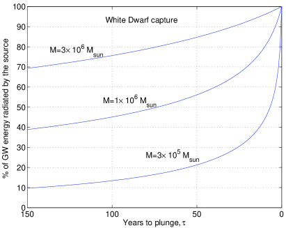
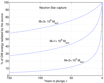
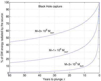
FIG. 11.: Percentage of GW energy radiated (out of the total energy radiated during the entire inspiral) as a function of the time $\tau$ left to plunge, for typical captures of a WD (upper left panel), a NS (upper right panel), and a BH (lower panel), for a range of MBH masses. The masses of the WD, NS, and BH are taken to be $m=0.6,1.4$, and $10M_{\odot}$, respectively, and in all cases the CO plunges at eccentricity $e_{\rm LSO}=0.15$. A substantial fraction of the energy is emitted long before plunge, when the source is still not detectable by LISA. This energy is mostly emitted in relatively high-frequency bursts near periastron passage, and so contributes to the confusion noise.

For such typical sources, the GWs emitted near plunge are in the LISA band, so one might naively have thought that the GWs emitted $10-150$ yr before plunge would be at frequencies well below the LISA band. But this is not true, since most of the radiation is emitted in relatively high-frequency bursts (i.e., high harmonics of the orbital frequency) near periastron passage. To illustrate this, in Fig. 12 we plot the signal from a WD captured by a $10^{6}M_{\odot}$ MBH at 1 Gpc. This plot shows the evolution of the signal during the last 1000 years of inspiral, as distributed among the first 20 harmonics of the radiation. We see that early in the inspiral history, the radiation is dominated by the high harmonics, which are well within LISA’s sensitivity band. Thus the capture source is effectively “in band” throughout the entire inspiral, and so is always a potential source of confusion.

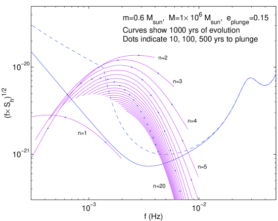
FIG. 12.: GW output from the last 1000 years of inspiral of a captured WD at 1 Gpc. Shown (solid convex curves) are the characteristic amplitudes $h_{c,n}$ [see Eq. 65] of each of the first 20 harmonics (labeled $n=1,\ldots,20$), for a capture of a $0.6M_{\odot}$ WD by a $10^{6}M_{\odot}$ nonspinning MBH, with plunge eccentricity 0.15. The signal curves are superposed on LISA’s instrumental noise (solid concave curve) and LISA’s noise curve including confusion from WD binaries (dashed curve). In each $h_{c,n}$ curve, the right end corresponds to the instant of plunge, the left end corresponds to 1000 years before plunge, and dots along the curve correspond (from right to left) to 10, 100, and 500 years before plunge. Note that even 500 years before plunge, most of the GW energy is radiated “in band”—i.e., in the frequency range where LISA is most sensitive. Although at such early times the orbital frequency is well “below band,” most of the energy radiated then is carried by high harmonics of the orbital frequency.

The second piece of input required for our estimate of subtractable noise is the SNR output from typical sources, as a function of $\tau$. Following Finn and Thorne [17] we write the two-detector (sky-averaged) SNR² as a sum of contributions from all harmonics of the orbital frequency:

$${\rm SNR}^{2}=2\,\Sigma_{n}\int\frac{h^{2}_{c,n}(f_{n})}{f_{n}S_{h}(f_{n})}\,d\ln f_{n},$$ (64)

where

$$h_{c,n}=(\pi d)^{-1}\sqrt{2\dot{E}_{n}/\dot{f}_{n}}$$ (65)

is the “characteristic amplitude”, $f_{n}=n\,\nu$, and $\dot{E}_{n}$ is the power radiated to infinity by GWs at frequency $f_{n}$, given, to lowest order, by Eq. (11) above. The results are shown in Fig. 13. In practice, we summed over the first $100$ harmonics. Also, we performed the integral in the time domain, using $\dot{f}_{n}=n\dot{\nu}$, with $\dot{\nu}$ given by the lowest-order formula, Eq. (62).

Of course, the SNR results we estimate this way cannot be very accurate, in general, since they are based on quasi-Newtonian orbits and lowest-order radiation reaction formulae. Their inaccuracy can be gauged, to some extent, by comparison with exact (to numerical accuracy) values obtained by Finn and Thorne [17] for the case of circular, equatorial orbits. For the last year of inspiral of a $10{M_{\odot}}$ BH into a $10^{6}{M_{\odot}}$ Schwarzschild MBH, and using essentially the same LISA instrumental noise curve that we use, but neglecting confusion noise, Finn and Thorne find the (sky-averaged) value ${\rm SNR}=72$ [28] for one synthetic Michelson. For the same case (and again neglecting confusion noise), our method estimates SNR = 105 (again, for one synthetic Michelson). Therefore our SNR is $45\%$ too high for this case. Unfortunately, for eccentric orbits, and even for circular orbits several years before the final plunge, there is no “gold standard” that we can compare our SNR estimates to. We shall assume that our SNR estimates are correct to within a factor $\sim 2$, and we shall see that this accuracy is good enough for drawing our main conclusions.

In the analysis below we shall assume that ${\rm SNR}_{\rm thresh}=30$, so sources are detectable out to an average distance $d_{\rm det}$ of

$$d_{\rm det}/(1{\rm Gpc})=\text{(average 3-yr SNR @ 1 Gpc)}/30,$$ (66)

where the 3-yr SNR is calculated as described above. However, given the various approximations and uncertainties (the rough nature of our SNR calculation, the uncertainty in our estimate of ${\rm SNR}_{\rm thresh}$, the fact that typical observation times might be $\sim 5$ or more years instead of $3$), we shall also point out how our results below would change if $d_{\rm det}$ were a factor two larger or smaller than our estimate.

    

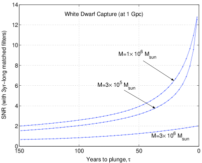
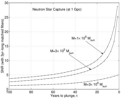
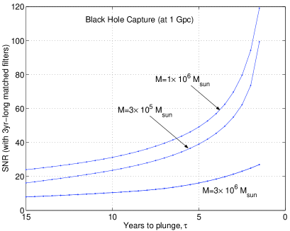
FIG. 13.: Combined SNR (from two synthetic Michelsons) as a function of time $\tau$ left to plunge for the three cases shown in Fig. 11, at a fiducial distance of 1 Gpc. Each SNR data point represents the matched filter SNR for a 3-yr-long waveform segment centered at $\tau$.

1 Subtracting the resolvable WD captures

In Sec. IV above we estimated the spectral noise density ${\cal S}_{h}^{\rm WDcapt}$ from all WD captures (see Fig. 6). What portion of this noise is subtractable?

Consider first WD captures that are completed (i.e, the WD is swallowed by the MBH) during the LISA mission lifetime ($\sim 3-5$ yr). From Fig. (13), we see that on average SNR$\sim 9$ for such captures, so from Eq. (66) we estimate $d_{\rm det}\sim 0.3$ Gpc. Since the proper-motion distance at $z=1$ is 3.3 Gpc, and since the contribution from sources at $z<1$ is around $85\%$ of the contribution from all $z$ (see the discussion in Sec. IV D above), we estimate that a mere $(0.3/3.3)\times 0.85\sim 8\%$ of the energy from the sources that plunge during LISA’s lifetime is subtractable.

Consider next the contribution to the confusion energy from captures that are not completed during LISA’s lifetime. Clearly, for these captures (which have a smaller 3-yr SNR, and so must be closer to us than $d_{\rm det}\sim 0.3$ Gpc to be detectable), the portion of subtractable energy will be even smaller than the above 8%. Let us attempt to estimate this portion, very roughly: Examining Fig. 13, we find that the 3-yr SNR from typical WD captures drops by a factor $\sim 5$ over the last $\sim 100$ years of inspiral. Thus WD captures with $\sim 100$ years to live can be detected out to an average $\sim 0.06$ Gpc. These detectable sources contribute $\sim 2\%$ of the capture noise (since this fraction scales as the detection distance), so averaging $\sim 2\%$ and $8\%$, we estimate that of all the capture noise from sources with $0-100$ years until final plunge, $\sim 5\%$ is resolvable. According to Fig. 11, however, these sources contribute, on the average, only around $55\%$ of the total confusion energy—the rest is attributed to captures that have more than 100 years to plunge when LISA observes. From the sources with $>100$ years to go until plunge, we similarly estimate that $\sim 1\%$ of the capture noise is resolvable. Hence, we estimate the overall fraction of subtractable energy from WD captures is roughly $0.55\times 5\%+0.45\times 1\%\approx 3\%$.

In conclusion, we estimate that $\sim 97\%$ of the capture noise from WDs represents an irreducible confusion noise:

$$S_{h}^{\rm WDcapt}(f)\approx 0.97\times{\cal S}_{h}^{\rm WDcapt}(f).$$ (67)

If we were to assume that $d_{\rm det}$ is twice as large as estimated above (say, because we have underestimated the signal strength, or the low-frequency noise is significantly better than the design goal, or the mission lifetime is much longer than 3 years, or because our estimate of ${\rm SNR}_{\rm thresh}$ was too pessimistic), then the fraction of subtractable energy would only increase to $6\%$. Clearly, in either case it is a good estimate to simply take $S_{h}^{\rm WDcapt}(f)\approx{\cal S}_{h}^{\rm WDcapt}(f)$. Of course, this last approximation becomes even better if $d_{\rm det}$ is smaller than estimated above.

2 Subtracting the resolvable NS captures

We next apply similar arguments to estimating the fraction $S_{h}^{\rm NScapt}/{\cal S}_{h}^{\rm NScapt}$ of unsubtractable noise from captures of NSs. Fig. 13 shows that NS captures with $\tau$ less than a few years can be detected to a distance $\sim 0.6$ Gpc— roughly twice as far out as for WDs. Therefore, the same reasoning as above for WDs suggests that roughly $16\%$ of the GW energy impinging on the detector from NS captures is resolvable and hence subtractable (i.e., twice the fraction we found for WDs). Examining Figs. 13 and 11 again, we find that captures that plunge $\sim 40$ years after LISA ends operations are detectable to a distance of $\sim 0.17$ Gpc, so $\sim(.17/3.3)*0.85\approx 4\%$ of the energy from these is subtractable. Estimating that half the NS confusion background comes from sources with $0-40$ years before plunge, and half from sources with $>40$ years, and estimating that the average subtractable noise portion for these two classes are $10\%$ and $2\%$, respectively, we find (very roughly)

$$S_{h}^{\rm NScapt}(f)\approx 0.94\times{\cal S}_{h}^{\rm NScapt}(f).$$ (68)

If we were to assume NS captures are actually detectable to twice the distance estimated above, we would still have $S_{h}^{\rm NScapt}(f)\approx 0.88\times{\cal S}_{h}^{\rm NScapt}(f)$. Clearly, as with the WDs, it is a good first approximation to simply take $S_{h}^{\rm NScapt}(f)\approx{\cal S}_{h}^{\rm NScapt}(f)$.

3 Subtracting the resolvable BH captures

From Fig. 13 we estimate that BH captures that plunge during LISA’s lifetime will have an average 3-yr SNR of $\sim 80$ at $1$ Gpc, and so will be visible to $d_{\rm det}\sim 2.7$ Gpc (so almost to $z=1$). Hence, unlike the situation with WDs and NSs, most of the energy from BH captures that plunge during LISA’s lifetime is probably attributed to resolvable sources, and hence is subtractable.

To estimate the confusion noise level we refer again to Figs. 13 and 11: BH sources with $\sim 10$ years to go before plunge are detectable only out to $\sim 0.7$ Gpc, so $\sim 80\%$ of the background from these sources is not subtractable. From Fig. 11, roughly $40\%$ of the GW energy is released more than 10 years before final plunge, and so (averaging $80\%$ and $100\%$, and then multiplying by $0.4$) we estimate that at least $\sim 35\%$ of the BH background is unsubtractable:

$$S_{h}^{\rm BHcapt}(f)\mathrel{\hbox{\hbox to0.0pt{\hbox{\lower 4.0pt\hbox{$\sim$}}\hss}\hbox{$>$}}}0.35\times{\cal S}_{h}^{\rm BHcapt}(f).$$ (69)

(Note the RHS is a lower limit, since here we have not included the hard-to-estimate contribution from unresolvable sources with $\tau<10$ yr.) If we instead assume $d_{\rm det}=1.4$ Gpc for BHs with $10$ years to go before plunge (i.e, twice what we estimated above), then the same steps yield $S_{h}^{\rm BHcapt}(f)\mathrel{\hbox{\hbox to0.0pt{\hbox{\lower 4.0pt\hbox{$\sim$}}\hss}\hbox{$>$}}}0.3\times{\cal S}_{h}^{\rm BHcapt}(f)$. On the other hand, if $d_{\rm det}$ is half what we estimated above, then $\sim 40\%$ of the energy from BHs that plunge during LISA’s operation will not be subtractable, and for sources with $\sim 10$ years to go before plunge, the unsubtractable fraction increases to $90\%$. Thus overall, the unsubtractable portion would be $\sim 75\%$ [$\approx 0.5(0.4+0.9)0.6+0.5(0.9+1.0)0.4$]; i.e., $S_{h}^{\rm BHcapt}(f)\approx 0.75\times{\cal S}_{h}^{\rm BHcapt}(f)$.

The above estimates were made assuming $S_{h}^{\rm BHcapt}(f)$ does not significantly raise the total effective noise level. However, if the BH capture rates are at the high end of the estimated levels, then $S_{h}^{\rm BHcapt}(f)$ does significantly raise the total noise curve, thereby reducing the distance out to which the BH sources can be resolved. Then $S_{h}^{\rm BHcapt}(f)$ would be in the intermediate regime shown in Fig. 10, where it is difficult to estimate without going through the entire recursive procedure described in Sec. V A.

For this reason, at the highest BH capture rates ($\kappa^{\rm BH}\mathrel{\hbox{\hbox to0.0pt{\hbox{\lower 4.0pt\hbox{$\sim$}}\hss}\hbox{$>$}}}3\times 10^{-7})$, our present work is simply too crude to place very restrictive limits on the ratio $S_{h}^{\rm BHcapt}(f)/{\cal S}_{h}^{\rm BHcapt}(f)$. Instead, we quote the following range

$$S_{h}^{\rm BHcapt}(f)=(0.3-1)\times{\cal S}_{h}^{\rm BHcapt}(f)$$ (70)

(noting that the upper end of this range would be approached only if the BH capture rate is very high, so that capture noise significantly raises the overall noise level) and leave it to future work to improve this estimate.

VI LISA’s total noise curve

Having estimated what fractions of the three CO backgrounds are not subtractable, we may finally plot their effects on LISA’s total noise curve $S^{\rm eff}_{h}(f)$. Figures 14–16 depict $S^{\rm eff}_{h}(f)$, as derived from Eq. (41), with the contributions from the different CO species (WDs, NSs, or BHs) considered separately. [Recall from the discussion around Eq. (41) that in the range $f\mathrel{\hbox{\hbox to0.0pt{\hbox{\lower 4.0pt\hbox{$\sim$}}\hss}\hbox{$>$}}}1$mHz, the effect of the capture confusion noise (like the ones of instrumental noise and EGWDB background) is effectively increased by a factor that counts the bandwidth lost when fitting the GWDBs.] In the case of WDs and NSs we have included all capture noise as confusion noise, since our above estimates suggest that the subtractable portion of the noise would be small for these sources. For BH captures we have assumed that $0.3$ of the capture noise is unsubtractable, but have also shown the extreme case where $S_{h}^{\rm BHcapt}={\cal S}_{h}^{\rm BHcapt}$ [see Eq. (70)]. For each species we also refer to two cases, corresponding to the lower and higher end of the estimated event rate for that species. Note that the astrophysical event rate remains the main source of uncertainty in our analysis, and clearly overwhelms the uncertainty introduced by our crude estimate of the ratio $S_{h}^{\rm capt}/{\cal S}_{h}^{\rm capt}$.

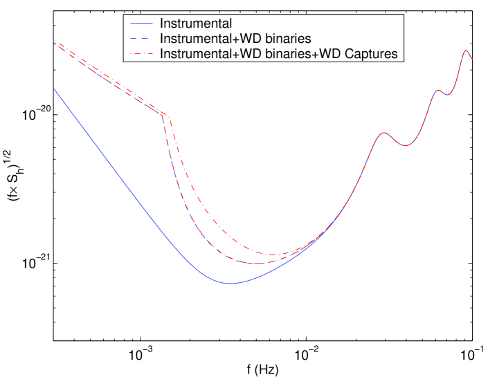
FIG. 14.: Total LISA noise (dash-dot line), including instrumental noise, confusion noise from WD binaries, and confusion noise from captures of only White Dwarfs. The two total-noise curves correspond to the higher and lower end of the estimated event rate for WD captures. (For the lower rate, the level of WD capture confusion noise is low enough that the corresponding total-noise curve appears to coincide in this plot with the dashed curve, representing instrumental and WD-binaries confusion noise only.) By virtue of Eq. (67), we have assumed here that the entire capture background ${\cal S}_{h}^{\rm WDcapt}$ contributes to the confusion noise $S_{h}^{\rm WDcapt}$. The total noise curve has been calculated using Eq. (41).

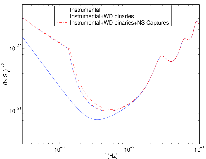
FIG. 15.: Same as in Fig. 14, but this time showing the total LISA noise when capture confusion from only Neutron Star sources is taken into account. By virtue of Eq. (68), we have assumed here that the entire background ${\cal S}_{h}^{\rm NScapt}$ contributes to the confusion noise $S_{h}^{\rm NScapt}$.

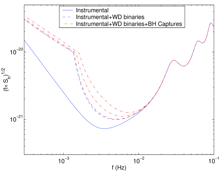
FIG. 16.: Same as in Fig. 14, but with capture confusion from only Black Hole sources taken into account. The three dash-dot lines show the total noise curve under different assumptions as to the event rate $\kappa^{\rm BH}$ and the fraction of the background that is subtractable. The lower total-noise curve refers to the lower end of event rate estimates ($\kappa^{BH}=6\times 10^{-8}$), with $S_{h}^{\rm BHcapt}$ assumed to be $0.3\times{\cal S}_{h}^{\rm BHcapt}$. The middle total-noise curve corresponds to the upper end of rate estimates ($\kappa^{BH}=6\times 10^{-7}$), again with $S_{h}^{\rm BHcapt}=0.3\times{\cal S}_{h}^{\rm BHcapt}$. The upper curve assumes the upper end of rate estimates, but with $S_{h}^{\rm BHcapt}={\cal S}_{h}^{\rm BHcapt}$. Thus the upper curve represents an upper limit on the effect of confusion noise from BH captures.

VII Summary, implications, and future work

We have seen that astrophysical rates for CO captures are either near (within one or two orders of magnitude) or at the point where confusion noise from these sources begins to dominate LISA’s noise curve. That is, basically, a good situation: Such event rates maximize the detection rate for these interesting sources. Moreover, even at the high end of estimated rates, LISA’s total noise level $[fS^{\rm eff}_{h}(f)]^{1/2}$ is raised by less than a factor $\sim 2$ by the CO capture confusion noise, so other LISA science (such as detections of MBH-MBH mergers) is not jeopardized.

Let us also highlight an important point that is implicit in Fig. 13: For WD capturess, HPOs will account for roughly half the detections. (Again, HPOs are “holding-pattern objects,” i.e., COs detected $10$ or more years before they plunge). To see this, in Fig. 17 we plot (in arbitrary units) the detection volume $V_{\rm det}$ times the time until plunge $\tau$, versus $\ln\tau$, for our fiducial sources. This uses the same information as contained in Fig. 13, since we have simply taken $V_{\rm det}\propto d_{\rm det}^{3}\propto({\rm SNR}@1{\rm Gpc})^{3}$; however, since the total number of detected captures (for each type of source) is proportional to $\int{V_{\rm det}\tau\,d\ln\tau}\,$, this representation allows one tell at a glance the relative importance of HPOs to the total detection rate. In particular, we find that $\sim 1/2$ of detected WDs and $\sim 1/3$ of detected NSs will have $\tau>10$ yr. While the BH detection rate will be dominated by sources with $\tau\mathrel{\hbox{\hbox to0.0pt{\hbox{\lower 4.0pt\hbox{$\sim$}}\hss}\hbox{$<$}}}3$ yr, $\sim 5-10\%$ of BH detections will have $\tau>10$ yr as well. [This last estimate is based on a linear extrapolation of the curves in Fig. (17) to larger $\tau$ values. Unfortunately, at $\tau\mathrel{\hbox{\hbox to0.0pt{\hbox{\lower 4.0pt\hbox{$\sim$}}\hss}\hbox{$>$}}}12$ yr, for the lower MBH mass, the BH orbits attain very high eccentricities ($e>0.9$), rendering our code unreliable.] Clearly, the results here are quite crude (most importantly, the results in Figs. 13 and 14 are all based on a single, fiducial value of the final eccentricity, $e_{\rm LSO}=0.15$), but still the moral seems to be clear: When searching over the large parameter space of possible capture signals, it will be worthwhile to construct template families that include waveforms from HPOs. We also point out that many of the HPOs that LISA detects will still be “alive” when some next-generation LISA is flown (and, for some of the WDs, next-next-generation LISA, etc.) which may allow for especially sensitive tests of GR in the future.

    

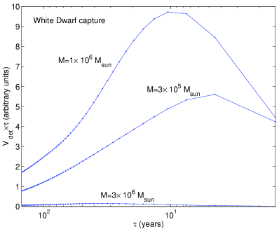
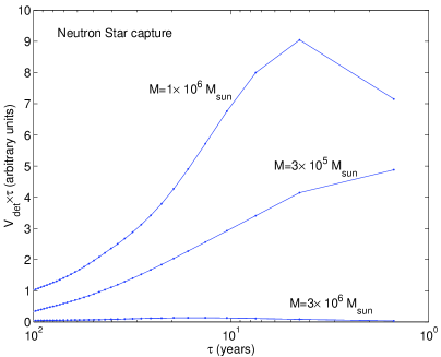
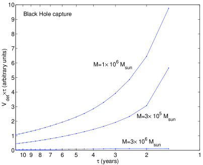
FIG. 17.: The detection volume $V_{\rm det}$ times $\tau$ (the time from the middle of the 3-yr observation until plunge), as a function of $\ln\tau$, for our three fiducial sources. The total number of detected captures is proportional to the integral $\int{V_{\rm det}\tau\,d\ln\tau}$. Roughly half (one-third) of the WDs (NSs) that LISA detects will have $\tau>10$yrs. BH detections will be dominated by sources with $\tau<3$ yr, but roughly $20\%$ will have $\tau>5$yr.

Clearly, the analysis in this paper has been crude in many ways. In particular, most of the estimates in Sec. V were based on taking results from a few fiducial cases, and then “averaging by eye.” Nevertheless, the uncertainties due to our approximations are clearly dwarfed by the uncertainties in the astrophysical rates. Moreover, our basic conclusion regarding WDs and NSs—that most of the GW energy we receive from these captures is not resolvable by LISA and so represents a confusion noise—seems very robust. For the BH case, our estimated range of $S_{h}^{\rm capt}$ is rather broader: $S_{h}^{\rm capt}\approx(0.3-1)\times{\cal S}_{h}^{\rm capt}$. However, here too, the basic moral remains clear: To raise LISA’s overall effective noise level by even a factor $\sim 2$, the BH capture rate would have to be at the high end of its estimated range, resulting in several hundred detections per year—a compensation devoutly to be wished.

- [1] J. R. Gair, L. Barack, T. Creighton, C. Cutler, S. L. Larson, E. S. Phinney, and M. Vallisneri, Proceedings of the Eighth GWDAW Meeting (Milwaukee, 2003); gr-qc/0405137.
- [2] J. A. Orosz, Proceedings of IAU Symp. 212, K. A. van der Hucht, A. Herraro, and C. Esteban Eds. (San Francisco, ASP, 2003); astro-ph/0209041.
- [3] M. Freitag, ApJ 583 L21 (2003).
- [4] M. C. Aller and D. Richstone, Astron. J. 124, 3035 (2002).
- [5] C. F. Gammie, S. L. Shapiro, and J. C. McKinney, Astrophys. J. 602, 312 (2004); J. C. McKinney and C. F. Gammie, astro-ph/0404512.
- [6] M. Freitag, Class. Quant. Grav. 18, 4033 (2001).
- [7] S. Sigurdsson, Class. Quant. Grav. 20 S45 (2003).
- [8] L. Barack and C. Cutler, Phys. Rev. D 69, 082005 (2004).
- [9] See, however, W. Schmidt, Class. Quant. Grav. 19 2743 (2002), which provides some analytic expressions for related quantities.
- [10] S. A. Hughes, Phys. Rev. D 61, 084004 (2000); Phys. Rev. D D64 064004 (2001).
- [11] C. W. Misner, K. S. Thorne, and J. A. Wheeler, Gravitation (San Francisco, Freeman, 1973), Eq. (33.32b).
- [12] C. Cutler, D. Kennefick and E. Poisson, Phys. Rev. D 50, 3816 (1994).
- [13] P. C. Peters and J. Matthews, Phys. Rev. 131, 435 (1963).
- [14] F. B. Estabrook, M. Tinto, and J. W. Armstrong, Phys. Rev. D 62, 042002 (2000).
- [15] http://www.srl.caltech.edu/shane/sensitivity/
- [16] K. Danzmann et al., LISA—Laser Interferometer Space Antenna, Pre-Phase A Report, Max-Planck-Institut für Quantenoptic, Report MPQ 233 (1998).
- [17] L. S. Finn and K. S. Thorne, Phys. Rev. D 62, 124021 (2000).
- [18] B. Abbott et al., Phys. Rev. D 69, 122004 (2004).
- [19] A. J. Farmer and E. S. Phinney, Mon. Not. Roy. Astron. Soc. 346, 1197 (2003).
- [20] G. Nelemans, L. R. Yungelson, and S. F. Portegies Zwart, Astron. and Astrophys. 375, 890 (2001).
- [21] P. L. Bender and D. Hils, Class. Quant. Grav. 14 1439 (1997).
- [22] S. A. Hughes, Mon. Not. R. Astron. Soc. 331, 805 (2002).
- [23] B. J. Owen, L. Lindblom, C. Cutler, B. F. Schutz, A. Vecchio, and N. Andersson, Phys. Rev. D. 58 084020 (1998).
- [24] E. S. Phinney, astro-ph/0108028.
- [25] E. S. Phinney, unpublished.
- [26] V. A. Sirota, A. S. Ilyin, K. P. Zybin, and A. V. Gurevich, astro-ph/0403023.
- [27] B. F. Schutz, in The Detection of Gravitational Radiation, D. Blair, ed. (Cambridge University Press, Cambridge, 1989).
- [28] K. S. Thorne, private communication.